Forecasting financial time series using multiple Kernel Learning

(1)

UNIVERSITAT POLIT`

ECNICA DE CATALUNYA (UPC) – BarcelonaTech

UNIVERSITAT DE BARCELONA (UB)

UNIVERSITAT ROVIRA i VIRGILI (URV)

FACULTAT D’INFORM`

ATICA DE BARCELONA (FIB)

FACULTAT DE MATEM`

ATIQUES (UB)

ESCOLA T`

ECNICA SUPERIOR D’ENGINYERIA (URV)

Forecasting Financial Time Series

Using Multiple Kernel Learning

Luis F´

abregues de los Santos

Master in Artificial Intelligence

Master’s thesis

Supervised by Argimiro Arratia

∗

and Llu´ıs Belanche

†

To be defended on 5/07/2017

∗_{Dept. of Computer Science, Universitat Polit`}_{ecnica de Catalunya} †_{Dept. of Computer Science, Universitat Polit`}_{ecnica de Catalunya}

(2)

(3)

Thanks to my tutors Argimiro Arratia and Llu´ıs Belanche for their insight on both Artificial Intelligence techniques and Financial theory. Their patience and proposals kept the project running.

Thanks to my friends Victor Grau and Armando D´ıaz for their ideas on caching partial results of the algorithms.

Thanks to my family, in particular my parents, for they support during this thesis and the entire mas-ter’s program.

Finally, thanks to my couple Sandra for cheering me up and being on my side during the days of in-tense work.

(4)

(5)

Abstract

This thesis introduces a forecasting procedure based on Multiple Kernel Learning to predict and measure the influence of several economic variables in the process of predicting the equity premium of the S&P 500 Index. In the experiments of Welch and Goyal they determined that, using linear models, those economic variables had an unreliable effect on the predictive capabilities of the models. The experiments performed in this thesis with MKL use the same data in an attempt to predict with non-linear models. The kernels that are part of the MKL procedure are multivariate dynamic kernels adapted for time series. The presented financial variables have a questionable impact on the predictive capabilities of the developed models due to the data being noisy. Some of the kernel methods for time series may not be able to extract any relevant information from exogenous variables, as they are matched in the results by a simple RBF kernel. MKL shows a poor capacity at selecting the best combination of kernels as it is also matched by RBF, and even the kernels that MKL uses. However the experimental results show that the presented methods have better predictive capabilities than the linear models.

Keywords

(6)

(7)

List of Figures

1 Multivariate Dynamic Time Warping. Source: [37] . . . 8

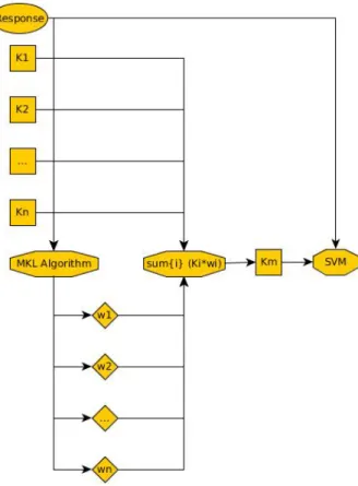
2 Multiple Kernel Learning general procedure. Ki are kernel matrices, wi are the weights computed by the algorithm, and Km is the combined kernel matrix. . . 13

3 Schema of the data preparation for this task. The first object(left) contains all monthly observations which are divided in yearly blocks of data(middle) to be part of windows of data points(right). . . 19

4 Weights of kernel methods with different MKL procedures for classification . . . 24

5 Weights of variables with different experimental settings using EasyMKL . . . 25

6 Weights of kernel methods with different MKL procedures for regression. . . 26

7 Weights of variables with different experimental settings using Kernel Alignment. . . 27

8 Ratio of over-fitting for all kernel methods . . . 32

(10)

(11)

List of Tables

1 The definition of the four experiments with their respective lags. . . 22

2 Results of kernel combinations using Out-Of-Sample Validation. . . 23

3 Results of kernel combinations using Cross-Validation.. . . 23

4 Resulting accuracies using exogenous variables. . . 24

5 Results of kernel combinations using Out-Of-Sample Validation. . . 25

6 Results of kernel combinations using Cross-Validation.. . . 26

7 Resulting errors using exogenous variables. . . 27

8 The definition of the data frames to test the variables. . . 31

9 The different factor levels for each decision of the Factorial Experiment. . . 33

10 The results of each experiment of the Factorial Experiment. . . 34

(12)

(13)

1. Introduction

Financial gain is probably the best incentive to spark research in the fields of mathematics and computer science. The biggest companies are in a perpetual cycle of self improvement, employing a vast amount of resources to make theoretical and practical developments to outplay their business opponents. Organiza-tions providing programming challenges offer enticing prices for the research teams that obtain the best solutions to their problems. Companies that have online presence hire the best researchers in the fields that may improve their internal algorithms. Being money such a successful motivator it is always interesting to research how the economies develop and, if possible, how these developments could be predicted.

Predicting the nature of the market itself has been the objective of much research by the statistics and machine learning groups. In particular the USA stock market returns have been used as data sets for these researches, as the number of recorded information of it is enough to apply learning techniques. The amount of information available does not make the problem easy however. The financial market is volatile, dependant on politics, natural disasters, and business movements.

One of the most representative indicators of the American stock market is the Standard and Poor's Index (S&P Index) and it has been the target of many prediction algorithms. Although the first approaches to this predictive task would only use lagged versions of this variable (just try to predict the S&P Index of tomorrow using the information of its past), soon researchers found new variables to add in to the predictive models. Those variables were shown to increase the capabilities of said models and perform well.

However, the improvement was spurious. Further tests using different data sets or slightly different techniques yielded unsatisfying results. The work performed by Welch and Goyal[40] offers a well-founded answer, concluding that the variables introduced by those other researchers yielded data and model depen-dent results. This put a slight stop to the creation and promulgation of these kind of variables, and the models using variables that are not the S&P Index.

The current situation holds a somewhat void of improvement in the use of exogenous(not S&P Index) variables. A common criticism to the work of Welch and Goyal is that they made use of mostly linear solvers to test those exogenous variables. On the other hand, newer non-linear approaches to this problem had been developed and tested with some degree of improvement using only the S&P Index. Very complex techniques such as Multiple Kernel Learning[21] have been applied to financial time series yielding good results, with the very interesting feature of providing a weighted vector to each of the input kernels, thus creating a comparison of influence between them in the final model.

There is a gap in the current literature as there are no methods that use complex non-linear solutions to exploit the exogenous variables. Non-linear models may unravel their importance or give another argument against their use. Variety of experimentation is key to this issue so employing several algorithms, method-ologies, and data representations is important to give redundancy to the results. Creating a document with said results may help in the present discussion.

The objective of this thesis will be to determine which is the best kernel learning method for these series and to ascertain what is the influence of the exogenous variables on the predictive models. The following work includes:

• A presentation of new kernels for time series with a comparative evaluation of them.

• An experimental procedure that uses the MKL technique to obtain a combined model and weights the composing kernels.

(14)

This document has the following sections: a State of the Art on which the most recent and insightful works on the field will be commented and analyzed, an introduction to the basics of kernel functions and kernels for time series on the Kernel Theory section, a short review of the kernel learning methods (including MKL) in the Kernel Learning section, an explanation of the data set which the experiments will be based on in the Experimental Data section, the main experimental procedure of the task will be presented in the Classification and Regression Experiment section, and the Exhaustive Experiment will describe more wide-range tests performed on the data.

Part from the work presented in this thesis was summarized in an article and accepted in the International Work Conference on Artificial Neural Networks (IWANN) in spring of 2017. The reference to the published article can be found at https://link.springer.com/chapter/10.1007%2F978-3-319-59147-6_16.

(15)

2. State of the Art

There is a long history of attempts to predict stock market returns by specifying a regression task using lagged predictor variables independent of the stock market returns. Shiller [34], Campbell and Shiller [7], Cochrane [11], among others, have studied the forecasting of future excess returns using the dividend price ratio as predictor. Other popular predictor variables explored in the literature are the dividend yield, earnings price ratio, dividend-to-earnings ratio, volatility, interest rates, exchange rates, consumption indices and inflation rates (see, e.g., [19], [24], [28], [29] and [13] for a general discussion). The list of valuation ratios sought of as forecasters of expected excess returns is much longer and show “... a pervasive pattern of predictability across markets wherein the cashflow or price change one may have expected is not what is forecast.” [13]. In view of this and further evidence showing the spurious nature of predictor models (mostly linear regressions on the aforementioned valuation ratios), several authors have conducted extensive studies on the forecasting performance of various economic variables and different models (to mention a few, e.g., [2], [6], [12], [40]). The work by Welch and Goyal [40] is of particular interest since the authors do a comprehensive revision of the empirical performance of the most widely accepted variables as predictors of equity premium, under linear regression models, and conclude that these models have poor predictive capacity both in-sample and out-of-sample.

Predicting the market returns has been the object of debate by practitioners given that the data is believed to be non-stationary and with a high degree of noise. The use of the previously mentioned predictor variables has often been a point of controversy given their unreliable results. Among common practises in investment, the ”buy-and-hold” strategy is based on buying stocks and holding them without regard of the market. This is further supported by the hypothesis of the efficient market(Fama [18]), which states that the market cannot be predicted and that no excess of return can be obtained by predicting the market.

Regardless of the efficient market hypothesis, many approaches to predict market returns have been developed. In particular, Support Vector Machine approaches with general kernels have been seen in the literature to create such predictive models (see, e.g., [17], [30], [27], [36]). These kernels are, however, not tailored to exploit the time dependency of the data. In this regard, the kernels created in [32] make use of said structures. The work exposed in [21] goes further into the complexity of the algorithms, employing Multiple Kernel Learning as a predictive model.

(16)

3. Kernel Theory

The following sections contain a brief description of kernels, the conditions they have to meet to be able to become a proper kernel, how a kernel matrix is defined and created, an introduction to kernels for time series, the many kernels for time series introduced in the literature, and a new kernel developed for this work.

3.1 Kernel basics

Kernels have various definitions depending on the context in which they are used. However, in this thesis, its definition will be the one most frequently used in the statistical machine learning field.

Kernels[25] are two-place symmetric functions that return the inner product of the arguments in some feature space, thereby inducing an implicit mapping that creates an image of the input into the desired feature space. It is then possible to compare input data in a higher-dimensional space without the need of calculating the exact coordinates of the transformation.

These functions are used in the task of dealing with data that cannot be related linearly. By using a kernel as a similarity measure the input data can be projected into a feature space in which it can be related linearly. The projection may be costly to be calculated however there are times in which it is not necessary, the kernel can be calculated using other methods. The technique to evade the actual mapping of samples is known as the ’kernel trick’ and it is widely used in machine learning applications.

Kernel functions can be defined as follows:

k(x,z) =hφ(x),φ(z)i (1)

where x,z ∈ X are input vectors. φ represents the mapping from the original feature space X into a new feature space F as follows:

φ:x →φ(x)∈F (2)

3.2 Kernel Matrices and Positive Semi-Definiteness

Using kernel functions it possible to create a kernel matrix [25]. These matrices are particular cases of Gram matrices, which are matrices of inner products of two data samples. In the case of kernel matrices this inner product is substituted by the kernel function. The formulation of the kernel matrix is as follows:

Kx = [k(xi,xj)]i,j∈I =      k(x1,x1) k(x1,x2) · · · k(x1,xn) k(x2,x1) k(x2,x2) · · · k(x2,xn) .. . ... . .. ... k(xn,x1) k(xn,x2) · · · k(xn,xn)      (3)

whereI is the space of indexes of all the samples.

Kernel matrices serve as the main data structure that will be used by the learning algorithms to create a model. It synthesizes the information of the input data and the information about the features of the data. It also serves as a validation method for the kernel function: any valid kernel function should produce a symmetric and positive semi-definite kernel matrices.

(17)

It is known that a function is a valid kernel function if and only if it induces positive semi-definite (p.s.d.) matrices [25]. Said property ensures that methods of convex programming will converge to a global solution using matrices created with those functions. This property is defined as follows:

n

X

i,j=1

cicjk(xi,xj)≥0 (4)

for all n ∈N,x1, ...,xn∈X andc1, ...,cn∈R.

This property can be applied directly to kernel matrices defined using a p.s.d. kernel. Any operation applied to a p.s.d. kernel matrix that does not alter that property will generate a viable kernel. Knowing that some basic operations like the sum, product and limit may not change this property (using positive operands), new kernels can be created applying such operations over existing kernels.

3.3 Kernels for time series

Time dependant data sets contain observations obtained with the same frequency. For instance, a data set can have the values of river saline levels measured monthly. This creates a homogeneity on the time stamps of each observation (they will always be separated by one month) but does not assure that a year, for example, will be complete. Failures on the measuring process may occur and the missing observation must be considered in a different way than typical missing data in other problems. The construction of kernels also considers these factors.

Kernels for time series can be constructed using two approaches: structural similarity and model sim-ilarity. Structural similarity employs methods to find an alignment of the data that makes possible the comparison between series. Model similarity changes the structure of the data by constructing a higher level representation of it and the comparison is performed using this new representation.

There are different philosophies on building time-dependant kernel functions. Two common approaches are: to build a kernel function around a previously defined model that takes into account the time depen-dency of the input data or to change the data in order to be used by existing and non-time dependant similarity functions. Both options will be explored on the particular models introduced below.

Identifying the structure of the series can be helpful to find the best method to define predictive models. A deterministic model works under the assumption that the data belongs to a determined function and uses numerical analysis techniques to fill missing values. This undefined function is considered as a combination of polynomial functions [22]. It is the simplest model that can be assumed in a time-series.

Real data sets are rarely deterministic, as the values usually deviate from a linear combination of functions. Models that take into account this consideration are called Stochastic Models. In this kind of model it is considered that future values depend on past values. This fact does not mean that Deterministic Models are useless in time series, but their limitations must be understood.

Determining if a model is deterministic or stochastic often follows an experimental approach: a model of the data is built using linear combinations of polynomial functions and the result is tested against the data. There are also mathematical procedures to determine if a data set follows a deterministic model, like in [4], in which they demonstrate the discriminant capability of a model based in singular value decomposition. The Lag and Autocorrelation plots can also help to distinguish between said models.

Stochastic models are very wide in definition and assume less information about the underlying data. Another assumption must be made in order to apply statistical models and, in the case of Stochastic

(18)

Models, that assumption is second order stationarity.

The definition of stationarity states that the distribution of data of an stochastic process is invariant in time. Also, the auto-covariance betweenXt andXt+τ only depends on the lagτ [31]. Given this definition

and assigning a value to the lag (which is the number of previous observations that should be taken into account to predict the actual one) it is possible to apply some probabilistic models to the data, assuming that the range in time defined by that variable is relevant.

On the other hand, Non-Stationary time series have their distribution moments change over time. The DickeyFuller test[16] can be used to detect if a data set is Non-Stationary. Another way to determine it is to plot the mean and the variance. If those values change strongly over time, the data might not be Stationary. That property can also be proven by notable changes in auto-covariance or spectrum values [31]. Box plots in particular can be useful to determine this.

Inside of Non-Stationary models, another assumption can be made in order to use statistical methods. A Seasonality model assumes that the properties of the data change through time with defined patterns. Seasonality can be detected by observing repeated patterns in the data, but that can be hard to ascertain. Some experts [26] prefer to fit a model that takes into account seasonality and assess if this characteristic was detected in the data.

Given that the context of the present work is financial time-series, it is generally understood that the data is not stationary, which makes theoretically nonviable the use of the immense majority of methods. A common practise is to work with successive differences of the series in order to make the data resemble a stationary process.

3.4 Vector Auto-Regression Kernel

Vector Auto-Regression(VAR)[20] is an econometric model that relates the data of the observation at point x(t) with a linear combination of lagged values of the observation. Each variable is defined by a function that represents its changes over a defined period of time using past information of itself and other variables. In order to fit a model, a lag parameter is provided, which defines how many time steps the function will be looking at in the past to assess the linear combination parameters. Vector Auto-Regression is a model by itself, capable of predicting values of new samples, but the information generated by it can also be used to create a kernel.

Vector Auto-Regression kernels can be built using three steps:

1. Build two VAR models with two series and fit them using a certain number of lags.

2. Append the values of the transition matrices and intercepts of each series and calculate the Frobenius norm over the difference of those values.

3. Apply the Radial Basis Function to the Frobenius distance to convert it to a similarity measure. The VAR model that relates the data of the observation at pointx(t) is the result of a linear combination of all the variables of the observation. The formulation is as follows:

x(t) =

L

X

l=1

(19)

where x(t) is the sample at time t, L is the number of lags of the model, A is the transition matrix (a square matrix with the same dimensions as features has the data), b is the intercept (a vector of the dimension equal to the number of features) and εt is the Gaussian noise at time t.

The VAR function can be used to build a model similarity kernel, as seen in [32]. In order to compare VAR models it is interesting to consider the transition matrices and the intercept vectors. A simple matrix can be built appending the intercept as an additional column of the transition. This results in

ˆ

B = (A1|A2|...|AL|[b]). In order to calculate the difference between seriess1 ands2 the difference between

ˆ

Bs1 and ˆBs2 is calculated and then the Frobenius norm is applied:

FD(s1,s2) =

r

Tracen( ˆBs1−Bˆs2)( ˆBs1−Bˆs2)T o

(6) Once this Frobenius distance is calculated, the distance can be transformed into a valid kernel using the Radial Basis Function(RBF) kernel:

kVAR =exp −FD(s1,s2) 2σ (7) The parameters of this kernel methodology are the number of lags L and σ. The value of L will be fixed to five. σ will be set to the median Frobenius distance between the time series being compared. Both these parameters are set following the indications of [32].

3.5 Global Alignment Kernel

Global Alignment(GA) is a generalization of a well-known family of distance and similarity measures called Multivariate Dynamic Time Warping(MDTW) introduced in [33]. In order to understand Global Alignment it is necessary to explain how MDTW works in the context of time series and which are its drawbacks.

The objective of Dynamic Time Warping is to measure the distance between two series. In order to do so, both series should be aligned. The core of the problem is to determine the best alignment between the two series and, using that alignment, measure their similarity.

An alignment in MDTW is represented by a set of relationships between a point in the series and another point of the same series or the other one. Considering s1 ands2 as two time series, those relationships are

the following: s1(t) withs2(t) denoted by →, s1(t) with s1(t+ 1) denoted by ↑ ands1(t) with s2(t+ 1)

denoted by%.

The relationships are represented as two integer vectorsπ1,π2of the same length with binary increases.

Each item of the vectors is a relationship between elements of the series. The length of the vectors is always equal to or less than the length of the smallest series. Each of the previously mentioned relationships can be represented on those vectors as follows: (0, 1) for →, (1, 0) for ↑ and (1, 1) for %. Intuitively, each vector π1(t) indicates an element of s1 that forms a relationship with the element π2(t) of s2. For the

sake of simplicity the two vectors that represent the alignment will be denoted asπ. Those alignments, by definition, only consider values of zero or one lag in both series.

After obtaining a satisfying alignment, the distance between the series can be obtained as follows:

Dπ =

|π|

X

i=1

(20)

Figure 1: Multivariate Dynamic Time Warping. Source: [37]

where the distance functiond can be any metric, most commonly the Euclidean distance.

The presented algorithm is capable of finding more than one alignment. The selected alignment will be the one that minimizes the distance between the series. The formulation of the final MDTW distance is as follows:

MDTW(s1,s2) =

1

|π∗|π∈minA(s1,s2)

Dπ(s1,s2) (9)

where |π∗| is the length of the alignment with less distance and A is the set that contains all possible alignments π.

This distance measurement does not fulfill the positive semi-definite requirement to form a kernel, even after applying the Radial Basis Function. For this reason the Global Alignment, explained in [15], generalization can be more widely applied, which delivers correct kernels and enables the creation of a structural similarity kernel.

Global Alignment follows the same computational steps as MDTW. However, instead of selecting the alignment with minimum distance, it considers all the alignments. This makes kernels defined by this metric positive semi-definite under mild assumptions. This is based on the notion that all alignments provide information about the similarities between both series.

The formulation of this kernel function can be expressed using several distance metrics. The following formula is the one used in the context of the thesis:

kGA(s1,s2) = X π∈A(s1,s2) e−Dπ(s1,s2)₌ X π∈A(s1,s2) |π| Y i=1 k(xπ1(i).yπ2(i)) (10)

(21)

where, k(s1,s2) = 1 2exp(− 1 σ2kx−yk2) 1−1₂exp(−_σ12kx−yk2) (11) where x and y are elements of s1 and s2 and σ is a parameter which is obtained from the adaptive

grid: σ ∈ {0.2, 0.4, ..., 2} ·median(kx(t1)−y(t2k)·

p

median(|x(t1|), wherex(t1) and y(t2) are samples

in the series. In [32] they use a rank-based approach to obtain that parameter. They retrieve the pair of observations at which the output variable variation reaches minimum in the series. This is an adapted formulation from the original proposed by [15] in which the points are chosen randomly.

An improvement over GA was introduced with the name of Fast Global Alignment or Triangular Global Alignment. This improved version aims toward reducing the computational time of the procedure. That is accomplished by using an extra parameter T that restricts the number of alignments taken into account during the final calculation of the kGA. In particular, lower values of T make the kernel function use

alignments close to the diagonal. Increasing the value of T increases the range of alignments that are taken into account.

3.6 Multivariate Dynamic Euclidean Distance Kernel

In the same line as Global Alignment Kernel the Multivariate Dynamic Euclidean Distance Kernel (MDED), introduced in [32] is a structural similarity model that creates an alignment of data between two series of different size in order to be able to compute the distance measure. MDED opts for a much simpler approach, as it removes the first elements of the longest series until it matches the size of the shortest time series.

Even if this alignment is potentially worse in most of the cases with respect to MDTW, MDED is computationally less expensive. The approach is also backed by financial theory: observations generated in later time stamps contain information from older ones.

Having that L16L2 whereL1 and L2 are the lengths of vectorss1 ands2 respectively, this alignment

is defined in the notation of MDTW as π1 = [0, 1, 2, ...,L1−1,L1] and π2 = [L2−(L1−1),L2−(L1−

2), ...,L2−1,L2]. Using said alignment, the calculation of the distance between the series is done as in eq. 8. Again, the metric employed is the Euclidean distance. In a similar line to the kVAR calculation, it

is necessary to calculate the RBF kernel using the defined dissimilarity measure in order to obtain a p.s.d. kernel: kMDED =exp −Dπ(s1,s2) 2σ (12) The parameter of this kernel function,σ is estimated using the median of allDπ of the available data,

as suggested in the work that introduces the algorithm [32].

3.7 Multivariate Dynamic Arc-Cosine Kernel

Arc-Cosine kernels have interesting properties[10]. Their behaviour is similar to a neural network with one infinite hidden layer. This kernel function can be defined using different degrees that have different properties with slim variations in formulation. In the authors define most of this properties and make an

(22)

experimental comparison of Arc-Cosine kernels with Radial Basis Functions. They obtain good results on challenging data sets, surpassing other SVM, and comparable results with deep belief networks.

The basic formulation of the Arc-Cosine kernel function depends on the angle between the samples. The angle between samples can be defined with the following formulation:

θ=cos−1 s₁Ts2 ks1kks2k (13) The formulation of the function is defined by the degree n, which regulates its complexity. The kernel function can be expressed as follows:

kn(s1,s2) =

1

πks1k

n_k_s

2knJn(θ) (14)

Jn is a family of functions that analyze the complex dependencies of the angle. The formulation is

quite complex for an arbitrary value ofn. However, in the context of this thesis, onlyn = 0 andn= 1 will be considered. The different formulations for both this degrees are:

J0(θ) =π−θ (15)

J1(θ) =sinθ+ (π−θ)cosθ (16)

Arc-Cosine kernels have different properties depending on the degree of the formulation, with many complex implications that can be found in the referenced work. This kernel function only has as parameter the degree,n, which has a small window of tuning. It makes that this kernel function has potentially bad results compared to other kernel functions that allow some parametrisation.

Arc-Cosine kernels as defined in [10] and, in the same line as the Euclidean Distance Kernel, are created to work with complete data. In order to work with time series an alignment must be used to obtain input data for the formula, thus creating a structural similarity model. The chosen alignment is the one presented in 3.6for its simplicity and re-usability.

(23)

4. Kernel Learning

After determining and forming the appropriate kernel matrix using the functions described in the previous section, a model is built to fit to the data and provide predictive capabilities. Kernel learning methods provide a process to create such models and tools to use them for prediction tasks.

The next sections will describe both general and particular kernel learning models: first a brief intro-duction on building Support Vector Machines for single kernels functions; second a conceptual description of Multiple Kernel Learning; and finally two particular MKL algorithms that will be employed in the tests.

4.1 Support Vector Machines

Support Vector Machines(SVM)[38] are predictive models. The learning algorithm in the case of classifi-cation is designed to create the biggest separation possible between samples of different classes. This is accomplished by creating a separating hyper-plane that divides the samples in two groups. The distance between this hyper-plane and the closest samples of each class is called margin and the algorithm max-imizes it. The samples that are in the margin are called support vectors and they define the shape of the hyper-plane. Similarly the regression techniques tries to create a hyper-plane that has the minimum distance to the samples as possible, considering a margin for errors.

The simplest formulation of this technique for classification is the following: min1

2w

T_w ₍₁₇₎

subject to

yi(wTxi +b)>1,i = 1, ...,m (18)

where w is the normal vector to the hyper-plane, b is the offset of the hyper-plane from the origin, x are the training samples and y are the training tags. The formulation of the regression problem[35] only changes the conditions of the equation of the classification problem:

yi −wTx−b 6ε

wTx+b−yi 6ε

(19)

where ε determines the maximum deviation from the function defined by f(x) = wt_x ₊_b _{to the}

samples. This formulation, however, does not allow non-linearly comparable data to be related correctly and the model is not influenced by the user with any parameter. In order to address those features,

ν-SVM[8] can be used for the classification problem:

min1 2w T_w ₋_νρ₊ 1 m m X i=1 ξi (20) subject to yi(wTφ(xi) +b)>ρ−ξi,i = 1, ...,m ξi >0,ρ>0 (21)

(24)

where ρ is a free parameter that serves as threshold, ξi are the residual errors and φ is a function that

maps the data to a higher dimensional space (a kernel in the context of this thesis). A similar formulation can be applied to the regression problem[9]:

min1 2w T_w ₊_C _νε₊ 1 m m X i=1 (ξi +ξi∗) ! (22) subject to (wTφ(xi) +b)−yi 6ε+ξi, yi −(wTφ(xi) +b)6ε+ξi∗ ξi,ξ∗i >0,i = 1, ...,m,ε>0. (23)

where C is the regularization parameter. ν is an interesting parameter in both problems. It serves both as an upper bound for the margin errors and a lower bound for the number of support vectors with respect to the number of training samples. Different values of this parameter can make the model behave in substantially different ways so its values should be chosen carefully.

4.2 Multiple Kernel Learning

Multiple Kernel Learning(MKL)[23] is a research field that aims to find the best combination of kernels to solve a task. It is possible for a problem to have several kernel functions that cover different characteristics of the data, or different representations of the same data. Those procedures create different kernel matrices that can be used to train a predictive model. However, it is also possible to combine the information of those matrices into a single combined matrix of kernels. MKL makes it possible to combine in the same predictive model information obtained using different techniques.

The mathematical formulation of this process is the following: kη(xi,xj) =fη(

km(xim,xjm) P

m=1|η), (24)

wherekη represents the combined kernel,fη is the combination (linear or non-linear) function,kmrepresents

a kernel function for a set of P kernels and η parametrizes the combination function. This particular formulation is for the case of the parameters of the combination function being fixed.

The combination functions of MKL procedures often obtain a vector of weights and perform a linear combination of the kernel matrices or functions weighted by the obtained vector. In order to infer the vector of weights, several approaches can be used. One of the most employed in practise is the optimization procedure by which the kernel weights are obtained using an optimization algorithm following a certain criteria. In the case of the convex sum of weights (all weights must be positive and sum one) the general optimization procedure is the following:

arg max

ω A(ωk,Y), (25)

where ω is the vector of weights, k is the list of input kernel functions, Y is the vector of response values andAis a similarity measure.

Two algorithms to perform this task are employed in the development of this work. EasyMKL, a classification approach of MKL based on the probability distribution of each class, and Center Alignment, a MKL algorithm for regression based on similarity measures between kernel matrices.

(25)

Figure 2: Multiple Kernel Learning general procedure. Ki are kernel matrices,wi are the weights computed by the algorithm, and Km is the combined kernel matrix.

4.3 EasyMKL

The EasyMKL[1] algorithm obtains the parameters of the combination function using an optimization approach, in particular solves a max-min problem involving the parameters of the combination function

η and the probability distribution of each class γ. After the η weights are obtained they are combined convexly (the optimization restrictions ensure that the weights are positive and sum one). The l-1 norm is used as a structural risk function to guide the optimization. As base learner it uses Kernel Optimization of the Margin Distribution(KOMD), a kernel classifier that performs direct optimization of the margin distribution.

The formulation of this approach starts with defining the convex combination: kη =

P

X

m=1

ηmkm, 06ηm61, (26)

where, in this case,ηm is the assigned weight to each kernel matrix. The initial optimization equation is:

max

η:kηk=1minγ∈ΓQ(η,γ) = maxη:kηk=1minγ∈Γ(1−λ)γ

T_y_ˆ₍ P

X

m

ηmkc_m) ˆyγ+λkγk2 (27)

whereλis an exogenous parameter of the optimization process, ˆy is the vector of training set classes and

c

(26)

the formulation of the problem can be simplified to: min γ∈Γ(1−λ) ˜η ∗_d η(γ) +λkγk22 (28) where, ˜ η∗= dη(γ)kdη(γ)k1 kdη(γ)k₂kdη(γ)k₂ (29) The implementation of this algorithm is quite simple, as a optimization MKL algorithm. The function to minimize is 28 subject to several constraints presented in the introduction of this technique. The authors also provide a pseudo-code for a greedy version of the algorithm in one of the appendixes for better comprehension.

As commented previously, the base learner is KOMD. That classification method is the internal proce-dure that the EasyMKL method uses for obtaining results and compute the optimized parameters. Com-mon implementations of this method include the capability of predicting values using the KOMD classifier. However, in the context of this thesis, the best procedure is using the parameters calculated by EasyMKL, calculating the combined kernel matrix, and using that matrix to train a Support Vector Machine. This makes the built system capable of more accurate predictions as the ν parameter is of capital importance for these kernels.

4.4 Center Alignment MKL

This algorithm performs kernel alignment using centered alignment[14], which is a similarity measure that can be used to compare kernel matrices. The first step in this procedure is to obtain centered kernel matrices, which are defined as each kernel matrix itself minus the expected value of the kernel function. Centering the features is a process that also centers the resulting kernel matrix which, in turn, improves the performance of the algorithm. Centering also solves previous problems with unbalanced data sets. This process effectively centers the feature mappings in the kernel. This transformation can be defined as:

kc = I−11 T F k I −11 T F , (30)

where I is the identity matrix, F is the number of features, 1 is a vector of ones of 1xF elements. kc

is positive semi-definite as it is defined as an inner product.

The MKL algorithm can be constructed using this formulation. Weights are calculated by maximizing the alignment between the combined kernel matrix and the target kernel matrix. The resulting weights can be calculated using simple quadratic programming optimization techniques. This particular formulation is for the convex version of the process:

˜ η∗ =argmax η∈η˜ ηTaaTη ηT_M_η , (31) where a= (hk1c,yyTiF, ...,hkPc,yyTiF) (32)

where ˜η is the set of possible weights with convex restrictions, a is a vector which represents the Frobenius distance between each centered kernel matrix to the response kernel matrix, M is a symmetric

(27)

matrix that contains the Frobenius distances for each combination of kernel matrices kjc and klc in j,l ∈

{1,P}. The implementation of this algorithm is also straight forward: equation 31 is introduced in a quadratic programming optimization algorithm with the problem constraints presented in the referenced work, obtaining the weights in the process.

(28)

5. Experimental Data

The experiments in this thesis use the same data as in [40] and are performed with a similar set of variables. It is a data set that comprises several financial features measured monthly, quarterly and yearly in the range of years between 1871 and 2005. It includes information from several sources, which will be commented besides the explanation of the features.

The objective of the work presented in [40] is to determine if several variables deemed by several researchers as predictors of financial returns have any real impact in general circumstances. The authors perform their experiment using mostly linear regression and comparing the impact of such variables under those models. Their objective is to compare all the variables fairly and determine which of them have an impact on the prediction of S&P 500 equity premium. They determine that all of them have questionable impact.

The objective of this work is to use a subset of those variables described in [40] with non-linear models. The data set offered by the authors of [40] contains many features, many more that is computationally possible to compare in the time frame for this thesis. For this reason, a selected set of features (either extracted or derived from the original data) will be employed in this work. What follows is the list of the terminology used for the target value and features, and a short description comparing them.

Target value

Equity Premium: A representation of the stock market returns, in this case of the S&P 500. It is calculated combining several features from the original dataept =log((Indext+D12t)/Indext−1)−log(Rfreet+ 1)

where Rfree is the risk-free rate. This feature is theoretically the return rate of an investment with zero risk, however in practice it is obtained from the interest rate of a three month U.S. Treasury bill. The variables associated with Index and D12 are the S&P 500 index and the dividends, respectively, and will be discussed in later sections.

Features

Stock Returns: The original problem uses S&P 500 index (also mentioned as SPX or simplyIndex) returns obtained from Center for Research in Security Press (CRSP) and the website of Robert Shiller. This variable encapsulates the market capitalizations of the largest public companies and serves as an indicator of the U.S. economy. In the context of this problem, SPX will be considered the endogenous variable.

Dividend Price Ratio: Both this feature and the following are dependent on the dividends(D12), which are a moving sum with a window of 12 months of the dividends paid on the S&P 500 index. The dividends data is obtained from the Shiller’s website and the S&P Corporation. The formula for the Dividend Price Ratio is dpt =log(D12t)−log(Indext).

Dividend Yield: Very similar to Dividend Price, but Dividend Yield considers past values of SPX dyt =log(D12t)−log(Indext−1).

Earning Price: In a similar line to the features created using dividends, earning price(E12) is the moving sum of earnings from S&P 500 index in a window of 12 months. Part of this data is extracted from Shiller’s website and the other part is the result from an interpolation process by the authors. The Earning Price is formulated asep=log(E12t)−log(Indext).

(29)

Stock Variance: It is a variable that encapsulates the sum of daily returns of SPX. This data was obtained by the authors with the help of G. William Schwert and CRSP.

Book-to-market ratio: It is the ratio of book value to market value for the Dow Jones Industrial Average. For the months from March to December, this is computed by dividing book value at the end of the previous year by the price at the end of the current month. For the months of January and February, this is computed by dividing book value at the end of two years ago by the price at the end of the current month. Book values from 1920 to 2005 come from Value Lines website.

(30)

6. Classification and Regression Experiment

As stated in the introduction, the objective of this work is to re-examine the experiments performed by Goyal and Welch in [40] with kernel functions and using multiple kernel learning to weight each feature in order to determine its relative influence in the prediction of the equity premium of SPX.

The experiment is divided in two tasks: regression and classification. The objective of the regression problem will be to predict as accurately as possible the equity premium of the next month. The classification task uses the sign of the equity premium of the next month instead. Positive values of this metric indicate good preconditions to hold a share and negative values indicate a proper time to sell those shares. The reason behind performing both these tasks is to provide a robust response to the usability of the proposed features.

The experimental process follows two phases. In the first phase only endogenous variables will be used. All the kernel methods will be evaluated individually and a Multiple Kernel Learning model will be built using those kernel functions as well. The objective of this first phase is to determine which method performs better in the prediction task. The second phase uses the exogenous variables over the best model of phase one. For each variable, a data frame is built and its influence on the result is observed using MKL. Different combinations of variables and lags will be used. All these experiments will be explained in the following sections.

Data Preparation

Kernel methods for time series do not work with the same data structures as general ones. Kernel functions as VAR or GA require data structures that are comprised of a window of observations in order to extract temporal relationships between them. Those data structures in this context will be blocks of a given size composed of sequential observations. The data compression process transforms the raw original financial information into several blocks of data. Knowing that the observation frequency of the data is monthly, an intuitive way of creating blocks is to build yearly data structures containing 12 observations each. Each of these blocks will be considered as a data point inside of the problem. Kernel matrices will be built applying the different kernel functions to each pair of data points inside of a set.

The sets of data points can be defined in several ways. The classical approach is to divide the available, labeled data in to three sets: a set to train the model, a set to validate the parameters and a set to test the model. Although this approach is very common and applicable to most problems, time series behaves in a different way. For instance, a common method to obtain these sets is using N-Fold Cross-Validation. In a time dependent problem this methodology allows to test a model with a set of data older than the data used to train the model, which is paradoxical. Leave-N-Out solves partially this problem but introduces a new one, which is the time difference between the set of data used to train the model and the set destined to testing. Trying to predict a result in the current year using data from seven years ago may result in misleading performance. Time dependent models are built considering that they should be evaluated with data of the near future. In order to reduce these effects a moving window approach will be employed.

In this thesis the moving window is defined as a set of data points with a fixed number of elements or years. After a window’s data is used to train, validate, and test a model the next window will start one year later with the same number of elements. This window will be divided inside the problem in train, validation and test sets. In order to respect the sequential nature of the problem only the last data point will be used as test data. Validation and train sets will contain a preselected number of samples, 2 and 20

(31)

respectively. The size of the window in this case is 23 (the sum of the elements of the three sets).

Figure 3: Schema of the data preparation for this task. The first object(left) contains all monthly obser-vations which are divided in yearly blocks of data(middle) to be part of windows of data points(right).

The output variable of this process varies depending on the task that is being evaluated. As introduced, the equity premium is the value to predict in the task of regression. The classification task uses only the sign to create a binary problem. The vector of the true output variables is computed before starting any model building and uses the value of the first month of the next year.

Working with time dependant models introduces an important dependency with past observations of the same variable. It is a common practise to include several lagged observations to increase the information provided to the model and form better temporal models. This practise will be applied to all the predictor variables, with different configurations and quantities of lags.

Performance Metrics

Metrics are strongly related to the type of task being performed. The results of a regression task are real values and they must be compared with the true value. In this case, the model will predict the equity premium of the following month and it will be compared with the true value. Mean Squared Error is a very common performance metric defined as:

MSE = 1 n n X i=1 (ˆyi−yi)2 (33)

Three different errors will be taken into account in the results: train error, validation error and test error. Test error measures the performance of the models against data out of sample, train error does the same for the in sample data and validation error helps to determine if the validation procedure is working correctly.

The performance metric selected for the classification task is the accuracy, defined as the number of correctly classified samples over the total number of samples. This simple metric is selected because it is

(32)

intuitive to use in classification problems and it is easy to compare models using it. This metric will also be applied to training, validation and test predictions.

The other metric employed to display results is the set of weights of the multiple kernel learning model. As stated in the definition of the work the weights of a multiple kernel learning can be helpful to determine the relative importance of each kernel. This metric will help to determine which kernel function creates the best models from the data and which kernel matrix, constructed with the different variables, has a higher impact on the prediction of the results.

Validation methods

The process of parameter tuning introduces a new data division problem inside each window, but with several changes with respect to the main approach. Having a concealed, small dataset for validation purposes results in destining only a few samples to predicting and obtaining performance metric for each parameter combination. Many implementations apply out-of-sample as a simple solution however there are arguments to also use K-Fold Cross-Validation. In this thesis, results produced by both will be reported. Although in past sections both these techniques have been discouraged, the problem to solve is not the same. In this section the algorithms will be used to find the best set of parameters for the final model so, using for instance Cross-Validation, does not build a model with future data, only uses it to find the set of model parameters.

The authors of [3] argue that the use of K-Fold Cross-Validation(CV) is possible under several circum-stances. In their work they state that this methodology is not used by many practitioners because it employs future data. The use of not-known data during the evaluation process can change the distribution of the resulting model and also alters the order of the observations when the folds are rearranged, eliminating natural relationships. However commonly used methods, as out-of-sample, do not use the available data in an efficient way. The research work performed in [3] suggest that the common effects of using CV are negligible under some conditions. Those conditions are:

• Independence between signals

• Stationarity of the distribution of the data

• The data must be used in an auto-regressive model

The authors also comment that their demonstration is applicable to other lagged non-parametric models. They demonstrate those claims by performing several experiments using data with different underlying distributions. The models increase their predictive capability using CV when the data is generated by an auto-regressive model. However, if the data is seasonal, CV performs worst that the rest of the models. Given the assumptions about the data that this thesis assumes it is only fitting to include both validation procedures and observe how they compare.

Methodology

The problem’s methodology is divided in two steps. The first is to determine which is the best single or combination of kernel functions to perform the described predictive task. The second is to use the selected method to determine the relative importance of each exogenous variable using the weights of the trained Multiple Kernel Learning model.

(33)

The first step follows the classical methodology of model comparison: perform a predictive task using the same data and compare the results using a predefined metric. The kernel functions defined in 3 will be used training aν-SVR or a MKL model. The results of each experiment will be shown in a comparative table. The process includes parameter tuning for each of the models. In the case of the single kernel functions, the creation and evaluation of the model is straight forward: a support vector machine is built and fitted using the training data and tested or validated with the rest of the data. In the case of Multiple Kernel Learning, all kernel functions introduced in 3 will be used to create several Gram Matrices that will become the inputs for the MKL procedure. The implementation of KernelAlign for regression lacks of a built-in method to perform predictions, for this reason the resulting weights will be used to create a combined matrix that will be the input to aν-SVR, which will become the predictive model. EasyMKL has an internal predictor, however the results are rarely good, as it lacks many of the parameters that Support Vector Machine permits. In a similar manner to the regression tasks, the combined kernel matrix can be feed to a ν-SVM and this methodology increases the predictive capability of the model. The method selected in this step will be considered as the internal method.

The second step tries to determine the relative importance of each exogenous variable by using the weights of MKL, the external method. The MKL must be feed with a list of matrices, each one containing a different variable combination. To create such matrices the procedure defines data frames, which are groups of yearly data containing different features. The input list to the problem contains one data frame for each of the five exogenous variables, one data frame with only the endogenous variable and one data frame with all the variables. The data frames containing exogenous variables also contain a certain number of lags of the endogenous variable. The result of the MKL procedure will generate a weight for each data frame, thus weighting the relative importance of each variable. Each data frame will contain the training and validation data for each internal method, creating a kernel matrix that will be included in the list of inputs to MKL. After the computation, the performance of the model can be measured using the predefined performance metric for each task and the distribution of weights.

Using this representation, the input of each experiment will be a list containing seven matrices encap-sulating the following features:

1. SPX

2. SPX and Dividend-Price Ratio 3. SPX and Earning Price 4. SPX and Dividend Yield 5. SPX and Stock Variance 6. SPX and Book-to-Market Ratio 7. All the features

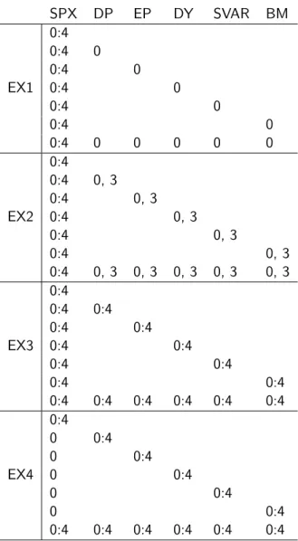
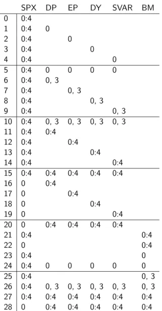
The experiments will be constructed including lagged versions of these features as additional information for the modeling process. Four experiments will be defined containing the seven data frames previously commented. Each experiment will be denoted by EX.

• EX1 only considers the exogenous variables without lags and SPX with four lags is included in each data frame.

(34)

SPX DP EP DY SVAR BM 0:4 0:4 0 0:4 0 EX1 0:4 0 0:4 0 0:4 0 0:4 0 0 0 0 0 0:4 0:4 0, 3 0:4 0, 3 EX2 0:4 0, 3 0:4 0, 3 0:4 0, 3 0:4 0, 3 0, 3 0, 3 0, 3 0, 3 0:4 0:4 0:4 0:4 0:4 EX3 0:4 0:4 0:4 0:4 0:4 0:4 0:4 0:4 0:4 0:4 0:4 0:4 0:4 0 0:4 0 0:4 EX4 0 0:4 0 0:4 0 0:4 0:4 0:4 0:4 0:4 0:4 0:4

Table 1: The definition of the four experiments with their respective lags.

• EX2 adds to the information of EX1 each exogenous variable with a lag of 3; this is motivated by the fact that the resulting data frame will contain more information but without adding too much redundancy.

• EX3 includes four lags of each exogenous variable.

• EX4 contains the same information as EX3 for the exogenous variables, but only includes the SPX without lags.

A visual representation of this data can be seen in table1.

6.1 Classification task

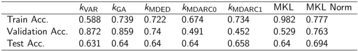
Tables 2 and 3 show the evaluation of the different kernel methods and multiple kernel learning using EasyMKL. These results are obtained using the same data for each method but adjusting the parameters

(35)

individually. The parameter ranges used in each of these methods can be found inA. All the methods are also include both parameter validation methods for comparison.

kVAR kGA kMDED kMDARC0 kMDARC1 MKL MKL Norm

Train Acc. 0.588 0.739 0.722 0.674 0.734 0.982 0.777

Validation Acc. 0.872 0.859 0.74 0.491 0.452 0.529 0.763

Test Acc. 0.631 0.64 0.64 0.64 0.658 0.64 0.694

Table 2: Results of kernel combinations using Out-Of-Sample Validation.

Train Acc. 0.61 0.762 0.742 0.675 0.729 1.000 0.898

Validation Acc. 0.751 0.691 0.674 0.559 0.445 0.417 0.568

Test Acc. 0.568 0.649 0.631 0.640 0.640 0.667 0.658

Table 3: Results of kernel combinations using Cross-Validation.

The results of this table have several interesting factors to cover. All of the test accuracy measures are in very defined range, between the 55% and 70%, which indicates the general capacity of Multivariate Dynamic kernels for this task. Individual kernels share similar test accuracy measures, around the 64%, including very simple kernels likekMDEDandkMDARC0. It is also worth to mention that the kernels based on

the arc-cosine kernel perform as well if not better than other more common kernel functions. In particular, kMDARC1 is the best performing individual kernel, surpassing Global Alignment in the version that uses

out-of-sample validation.

By a considerable margin, the best performing method is the combination of kernels created with EasyMKL, surpassing all the individual kernels. This technique tends to over-fit, as it can be observed in the difference of accuracy between training, validation and testing. It is most prominent in the case of cross-validation, were training accuracy is much higher than test and validation accuracy measures. The normalization (scaling individual kernel matrices to have the l2 norm) also has interesting repercussions on the results: it reduces training accuracy and increases validation accuracy, reducing over-fitting. The results of the normalization technique seem to differ depending of the validation technique employed.

Finally, it is also worth to comment the effects of the different validation techniques on the results. There is no clear pattern to determine if cross-validation selects better or worse models than out-of-sample since all kernels react different to this parameter tuning technique. In the cases ofkGA and not-normalized

MKL the results improve, but in the rest of kernel functions have the same or worst test accuracy. The results clearly differ with [3], specially in the case ofkVAR.

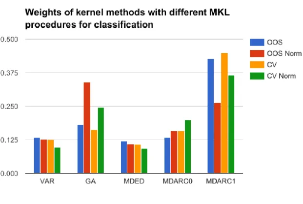
Figure 4 shows the resulting weights of the process of EasyMKL. It can be an interesting source of information to visualize how the algorithm determines which kernels are relatively more important.

From the results it can be observed thatkMDARC1 usually is the kernel with most weight. This further

supports the fact that this kernel function is possibly the best performing one for the problem. However, in the case of MKL with out-of-sample validation and normalization,kGAis the kernel with highest weight and

this combination is also the one with higher test accuracy. kMDARC0 also receives weights higher than the

mean, signaling that it is also important in the construction of the model and adds additional information. Finally, it is worth to comment the impact of the normalization in the weights: in all the cases it decreases the weights of kVAR andkMDED, the worst performing kernel functions.

(36)

Figure 4: Weights of kernel methods with different MKL procedures for classification

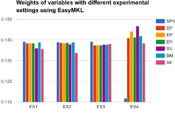
Figure6.1reflects the different weights obtained with the MKL process. All the experiments are executed using the best performing kernel method for the data, normalized multiple kernel learning using out-of-sample validation technique. Each variable is contained in a data frame that will be transformed into a kernel matrix using the MKL procedure.

Train Acc. Validation Acc. Test Acc.

EX1 0.757 0.767 0.574

EX2 0.764 0.772 0.567

EX3 0.758 0.784 0.600

EX4 0.733 0.779 0.533

Table 4: Resulting accuracies using exogenous variables.

The best performing method is EX3 in terms of test accuracy. EX1 and EX2 are fairly similar, indicating that the inclusion of the third lag does not affect too much the model. EX4 is the worst performing one, which can mean that the model heavily rely on the lags of SPX to predict the output. The weights of EX1, EX2, and EX3 are near the mean, with slightly higher weight for the endogenous variable. This result does not mean that the rest of variables are not important to predict the result (that will be represented with weights near zero) but that they are mostly equally important. EX4 has its weights shifted towards the exogenous variables. As those data frames lack of lags of SPX it is possible that the information contained in the exogenous variables takes a more active role in the prediction procedure, however the model performs worse in comparison to the rest. It is also worth noting that stock variance is still one of the most relevant

(37)

Figure 5: Weights of variables with different experimental settings using EasyMKL

variables in this case.

6.2 Regression task

Tables5and6shows the evaluation of the different kernel methods and multiple kernel learning using Center Alignment. These results are obtained using the same data for each method but adjusting the parameters individually. In all the methods the impact of using out of sample validation and cross-validation is also tested. All the methods are validated in the same range of parameters. For C and ν the available values are 0.2, 0.4, 0.6, 0.8, and 1. The range ofσ is 0.5, 1, 1.5, and 2.

Train MSE 0.0140 0.0029 0.0039 0.0045 0.0015 0.0032 0.0132

Validation MSE 0.0269 0.0119 0.0171 0.0137 0.0355 0.0091 0.0140

Test MSE 0.0472 0.0295 0.0326 0.0304 0.0645 0.0252 0.0351

Table 5: Results of kernel combinations using Out-Of-Sample Validation.

Mirroring the results of the classification task, the results of regression fall in a determined range that states the capabilities of these methods in the economic prediction tasks. The test errors are in the range between 0,02 and 0,07. In these results higher differences can be observed between the performances of different methods, with some methods being nearly thrice more accurate than others. Simpler methods

(38)

Train MSE 0.0122 0.0014 0.0015 0.0030 0.0009 0.0017 0.0109

Validation MSE 0.0305 0.0141 0.0184 0.0172 0.0326 0.0106 0.0184

Test MSE 0.0434 0.0265 0.0297 0.0275 0.0618 0.0251 0.0313

Table 6: Results of kernel combinations using Cross-Validation.

likekMDED andkMDARC0 perform relatively good howeverkMDARC1 has worse results than the rest of the

methods, probably attributed to over-fitting looking at the training error.

The best performing technique is the MKL, as it was in the classification case. A clear case of over-fitting can also be observed in this case considering the difference between the training error and the testing error. The parameters have been optimized using a shallow range of values so a fine tuning of them may reduce this effect. The normalization technique only increases the error of the methods, indicating a lose of information during this process.

The different validation techniques have a revealing impact on the regression task. As it can be observed on the tables, the results obtained using cross-validation as a parameter validation technique are always better than the result of OOS. This indicates that this technique is certainly useful for the validation process of the regression task. The results clearly support [3], contradicting the conclusions reached in the classification task.

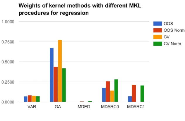
Figure 6: Weights of kernel methods with different MKL procedures for regression.

(39)

source of information to determine how the algorithm evaluates which kernels are relatively more important. From the results can be observed that kGA obtains the higher percentage of weight in all of the variations

of the experiment, with even higher values in the best performing settings of MKL. This fact is reinforced by the better results obtained by this kernel in the individual tests. The normalization procedure impacts the weights by making their values be more similar to the mean and assigning a much higher weight to kMDARC1. These results for kMDARC1 are opposite to the ones in the classification task, which indicates

how much these tasks are different. kMDARC0 has a significant impact on the resulting vector of weights,

which further mirrors the individual results.

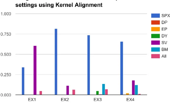
The table 7 and the figure 7 contain the experiments performed with exogenous variables and their results. All the experiments are executed using the best performing kernel method for the data, non-normalized multiple kernel learning using the cross-validation technique. Each variable is contained in a data frame that will be transformed into a kernel matrix using the MKL procedure. The parameter ranges remain unchanged in these results.

Train MSE Validation MSE Test MSE

EX1 0.0025 0.0129 0.0321

EX2 0.0024 0.0131 0.0332

EX3 0.0024 0.0131 0.0332

EX4 0.0024 0.0135 0.0344

Table 7: Resulting errors using exogenous variables.

(40)

The best performing method in the regression task for these parameters is EX1 in terms of test MSE. There is not much difference between the four experiments in their results, with EX1 being slightly better than the rest. It is noteworthy that all the results are worst than the versions without the exogenous variables. On the other hand, the weights are somewhat different. The SPX index is clearly the feature that most weight has in most of the variations of the problem, ranging between 60% and almost 80%. EX1 is an interesting result, as it has more weight to the Stock Variance than the SPX. This experiment also has the best results in the test set, however those results are bad in comparison to the errors of the endogenous variable. Given those results it seems that the regression task does not give any relevant weight to the exogenous variables in most of the cases, it relies mostly on the SPX feature to carry the prediction task. It is possible that the stock variance has interesting implications on the predictive capabilities, but the results contradict that statement.

Conclusions

The results indicate that, in this experimental procedure, the exogenous variables have a questionable importance in the predictive models. In the case of the classification task the weights are comparable between them, however this means that there is not a clear variable affecting the model more than others. The regression task yields different results, given high weights to the endogenous variable. The overarching conclusion in these results is that exogenous variables do not seem to increase the predictive capabilities of the model. Furthermore, in some cases, they worsen it.

The instability of these results is reported clearly in [40]. Not only the results are worst with the introduction of exogenous variables, but the weights also fluctuate with each different configuration of lags and variables. This can also be attributed to the capabilities of MKL as a learning model. The problem of over-fitting was present in both tasks, reporting low train error measures contrasted by high error scores in the validation and the test sets.

This experimentation concludes that introducing exogenous variables in this procedure does not increase the predictive capabilities of the model. Left to discuss is whether this result is the best that can be obtained from the data or if the reason behind the relatively bad results are the capabilities of the models.