An Evaluation of Training Size Impact on
Validation Accuracy for Optimized Convolutional
Neural Networks
Jostein Barry-Straume
Southern Methodist University, [email protected]
Adam Tschannen
Southern Methodist University, [email protected]
Daniel W. Engels
Southern Methodist University, [email protected]
Edward Fine
University of California, Berkeley, [email protected]
Follow this and additional works at:
https://scholar.smu.edu/datasciencereview
Part of the
Categorical Data Analysis Commons
,
Numerical Analysis and Scientific Computing
Commons
, and the
Statistical Models Commons
Recommended Citation
Barry-Straume, Jostein; Tschannen, Adam; Engels, Daniel W.; and Fine, Edward (2018) "An Evaluation of Training Size Impact on Validation Accuracy for Optimized Convolutional Neural Networks,"SMU Data Science Review: Vol. 1 : No. 4 , Article 12. Available at:https://scholar.smu.edu/datasciencereview/vol1/iss4/12
An Evaluation of Training Size Impact on Validation
Accuracy for Optimized Convolutional Neural Networks
Jostein Barry-Straume1, Adam Tschannen1, Daniel W. Engels1, Edward Fine2
1 Master of Science in Data Science, Southern Methodist University,
Dallas, TX 75275 USA
2 UC Berkeley School of Information, Berkeley, CA 94704 USA
{jbarrystraume, atschannen, dwe}@smu.edu [email protected]
Abstract. In this paper, we present an evaluation of training size impact on validation accuracy for an optimized Convolutional Neural Network (CNN). CNNs are currently the state-of-the-art architecture for object classification tasks. We used Amazon’s machine learning ecosystem to train and test 648
models to find the optimal hyperparameters with which to apply a CNN towards the Fashion-MNIST (Mixed National Institute of Standards and Technology) dataset. We were able to realize a validation accuracy of 90% by using only 40% of the original data. We found that hidden layers appear to have had zero impact on validation accuracy, whereas the neural density of the network and the chosen optimization function had the greatest impact.
1 Introduction
Machine learning has “emerged as the method of choice for developing practical software for computer vision” [1]. By the same token, image recognition is one of the top ten use-cases for machine learning [2]. CNNs are the current state-of-the-art model architecture for image classification tasks [3].
Andrew Ng puts forth that Strategic Data Acquisition (SDA) is a defining principal approach of an AI company, as it enables a defensible business model [4]. SDA involves creating a positive feedback loop wherein a foundational amount of data is collected, from which a product is born, and subsequently used by users whom produce more data for the company and their product [4]. Moreover, SDA is a
“multiyear chess game to acquire the data asset that allows you to build a defensible business” [4]. With this in mind, we are interested in determining the minimum amount of data needed with which to develop a reasonably accurate CNN.
The dataset of hand written digits developed by the Mixed National Institute of Standards and Technology (MNIST) is the most popular dataset for benchmarking the performance of Convolutional Neural Networks (CNNs) [5]. However, MNIST dataset is overused, easily solved, and no longer representative of modern computer vision tasks [6]. For these reasons, the next-generation Fashion-MNIST dataset is chosen as the vehicle with which to test the effects of training data size on the validation accuracy of a CNN. Specifically, given a greyscale image of a piece of
clothing and a validation accuracy of 90%, minimize the training data size for a Convolutional Neural Network (CNN).
Accomplishing this optimization problem necessitates subsetting the data into training, validation, and test sets. The shuffled and split data is used to train a CNN. The validation set is used for the purposes of tuning hyperparameters of the model. The CNN has various componential layers that are employed to find the minimum epochs for training, as well as minimum error in accuracy.
The main components of a CNN are the convolutional, pooling, and dense layers. The convolutional layer extracts feature selection and learning from given clothing images. The pooling layer reduces dimensionality to prevent overfitting and increase computational performance. The dense layers compute the weights for each node of the 10 labels in order to perform image classification.
Optimization of the training data size is realized through two metrics. The model checkpoint provides a metric wherein a loss function is monitored throughout epoch training. If the given loss function does not improve, then the model is saved as the best model. The early stopping method halts training if the given loss function being monitored has not improved from the previous epoch. Utilizing both the model checkpoint and early stopping method maximizes accuracy while simultaneously minimizing training time for the CNN.
Using only 40% of the original data as a training set, we were able to achieve a 90% validation accuracy on the Fashion-MNIST dataset. There is a decreasing rate of return with respect to validation accuracy as training set size increases. Moreover, there was no quantile overlap between validation accuracy group means of using 10% versus 25% of the original data for training.
With regards to CNNs being applied to the Fashion-MNIST dataset, there is strong statistical evidence to suggest that training set sizes cause differences in group means among validation accuracies. The p-value from our one-way analysis of validation accuracy variance is less than 0.0001, which is statistically significant at the alpha level of 0.05.
The remaining sections are organized as follows. In Section 2 we present a brief history of neural networks, the components of neural networks, and the metrics with which to analyze and compare their performance. We explore some of their applications and best practices in Section 3. The Fashion-MNIST dataset is presented in Section 4. The results are presented in Section 5, and we present our analysis of the in Section 6. Ethical concerns in regards to object recognition and CNNs are highlighted in Section 7. Lastly, we draw the relevant conclusions in Section 8.
2 Neural Network History, Components, and Metrics
2.1 History of Neural Networks
Neural networks can be traced back to a paper written in 1943 by Warren McCulloch
and Walter Pitts titled “A logical calculus of the ideas immanent in nervous activity”
modeled how human neurons operate by constructing electrical circuits [7]. An
important concept of human learning is highlighted by Donald Hebb’s “The Organization of Behavior” in 1949, whom emphasizes that a given neural pathway becomes stronger when a pair of nerves fires simultaneously [7]. In the 1950’s, IBM
researcher Nathaniel Rochester attempts creating a hypothetical neural network (NN) [7].
However, it was not until 1959 at Stanford that the first successful neural network is created [7]. Stanford’s Bernard Widrow and Marcian Hoff utilized Multiple
Adaptive Linear Elements, from which would inspire the names of their two NN models [7]. The first being ADALINE, which recognizes binary patterns for the purposes of bit prediction [7]. The second, MADALINE, expanded upon ADALINE and applied adaptive filtering to solve real-world problems with regards to echoes during phone calls [7]. Further advancements of NNs are made by 1962 by Widrow and Hoff upon creation of weighting connections between neurons [7].
The field of study pertaining to NNs is further expanded in 1975 as the first unsupervised NN is developed [7]. In 1986, David Rumelhart of Stanford developed the idea of backpropagation [8]. Rumelhart’s accomplishment was done so standing
on the shoulders of Widrow and Hoff, as he extrapolated their work and applied it to multiple layers [8]. Increases in computational power have given rise to more sophisticated models in recent times, such as Long-Short Term Memory (LSTM) [9].
2.2 Convolutional Neural Network Components
Current state-of-the-art model architecture for image classification tasks, CNNs are comprised of three components [10]. To enable classification, CNNs employ a series of filters to the raw pixel data of an image for extraction of feature selection after learning [10]. The first component of a CNN is its convolutional layers.
Convolutional layers apply a given number of convolutional filters to the given image [10]. The convolutional layer carries out a set of mathematical operations for each subregion of the image [10]. The resulting outcome is a singular value produced in the output feature map [10]. Additionally, a rectified linear units (ReLu) function is applied by the convolutional layers to introduce nonlinearity to the model [10].
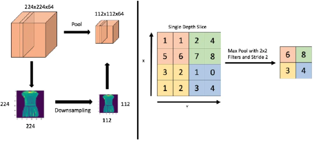
The second component is max pooling layers which are inserted in between convolutional layers in a CNN architecture [11]. Pooling layers function by downsampling the given image data extracted by the convolutional layers and reduce the dimensionality of the image. Put differently, for a given pixel tile extracted from the convolutional layer, max pooling distills subregions of the pixel tile containing the maximum values of the subregions. By doing so, multiple benefits for the model are realized. The spatial size of the images is reduced to minimize computation time [11]. Consequently, the number of parameters for feature selection is minimized as well [11]. In turn, the model avoids overfitting by narrowing the scope of parameters being selected [11]. Figure 1 illustrates the process of max pooling via downsampling.
Fig. 1.Left: Illustration of 2x2 Downsampling. Right: Diagram of Max Pooling.
The third component is a fully connected dense layer, which is incorporated into the last layer of the Convolutional Neural Network. It is this layer which performs the classification on the features extracted by the convolutional layers [3]. A softmax activation function is applied in the last layer to generate values between 0 and 1 for each node [3]. The values produced by this function given weights as to the probability of a given image falling into a certain classification [3]. The weights of these nodes are used to classify the given image. Figure 2 reflects a diagram of a neural network and the dense connectivity between nodes of each of its layers.
Fig. 2. Dense Layers of a Neural Network.
2.3 Convolutional Neural Network Metrics
Two main metrics are used to discover the minimum amount of training data size needed to meet a validation accuracy of 90%. Both metrics are enabled by the
creation of a validation set as Section 4.3 overviews as part of preprocessing. The first metric used to discern the optimal CNN is the model checkpoint. This function saves the given model being trained after every epoch if a new minimization of the monitored loss function is found [12]. The loss function that is monitored by the model checkpoint is mean squared error (MSE) [12]. Formula 1 details the exact methodologies for calculating the MSE in the loss function.
(1) The second metric used is the early stopping method which halts training when minimization has failed to iteratively improve based on the given absolute minimum delta. With a patience value of zero, the early stopping method will not wait between epochs to stop training if its loss function does improve. Like the model checkpoint, the early stopping method employs the MSE as its loss function to monitor.
3 Neural Networks Use Cases and Best Practices
3.1 Neural Network Use Cases
Neural networks (NNs) enable relationship understanding between independent and dependent variables, as well as abstraction of generalized patterns and behaviors [10]. With its hidden layers acting as feature selectors, and its last layer acting as a logistic regression classifier, problem domains of NNs range from linear, non-linear, and classification [10]. Unlike humans, NNs never tire or become bored, and as such are well suited for repetitive tasks [10]. In particular, identifying product defects via image classification on assembly lines is one such issue. Moreover, disease prediction
is another field that is aided by NNs’ ability to classify images.
Beyond image classification, NNs are capable of predicting weather forecasts and stock prices with data that is time-serial in nature [10]. Furthermore, neural networks have the ability to process sequential data to predict the next character in a given Internet search query, or the next sequence in a song or voice command [10].
3.2 Neural Network Best Practices
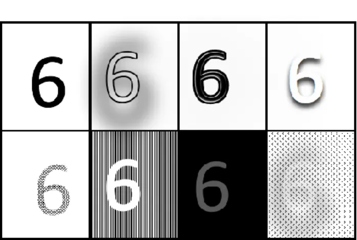
Microsoft researchers Patrice Y. Simard, Dave Steinkraus, and John C. Platt put forth two main best practices with regards to image analysis via neural networks. Firstly, Simard et al. found that increasing the size of the training set was in part responsible for optimal results [11]. In particular, expansion of the training set was realized by means of elastic distortion. New images are derived from the existing images by pixel distortion and obfuscation. As a result, the model constructed by Simard et al. was able to generalize to a better degree, and thus produce more accurate predictions on real-world datasets [11]. Figure 3 shows multiple examples of distortion techniques in order to achieve a larger dataset via augmentation.
Fig. 3. Examples of distortion techniques resulting in an augmented dataset.
The second-best practice asserted by Simard et al. for image analysis with neural networks was simply to use the best performing model; Convolutional Neural Networks (CNNs). The benchmarking performed by Simard et al. reflect that CNNs are more accurate than standard neural networks because of knowledge exploitation that inputs from a given image are not independent, but rather come from a spatial structure [11].
Another best practice for neural networks is to make use of drop out techniques. Nitish Srivastava et al. present dropout as a simple vehicle with which to prevent neural networks from overfitting [12]. Srivastava et al. showed that “dropout
improves the performance of neural networks on supervised learning tasks in vision, speech recognition, document classification and computational biology, obtaining state-of-the-art results on many benchmark datasets” [12]. Dropout is a method of randomly dropping nodes, along with their respective neural connections, from the neural network during training [12]. Consequently, the situation that Donald Hebb highlights in his 1949 paper is avoided. Specifically, arbitrary pairs of neural pathways are not over-emphasized by repeated connections.
4 Fashion-MNIST Data Collection
4.1 Fashion-MNIST Data History
MNIST stands for the Modified National Institute of Standards and Technology. The original MNIST dataset is a collection of handwritten digits gathered and created by Yann LeCun, Corinna Cortes, and Christopher J.C. Burges [13]. Its authors perpetuate it as a good dataset for which to conduct machine learning and pattern recognition techniques without involving heavy efforts in data preprocessing [13]. Because of the
The Fashion-MNIST dataset is the resulting culmination of a research project by Dr. Kashif Rasul and Dr. Han Xiao of Zalando Research [9]. Their reasons for creating a direct replacement of MNIST are threefold.
Firstly, Rasul and Xiao argue that MNIST is too easily solved now-a-days [9]. A publicly available Github Gist by David Robinson overviews comparing pairs of MNIST digits based on one pixel [14]. The capability to distinguish a pair of MNIST
digits utilizing simply one pixel lends credence to Rasul’s and Xiao’s assertions.
Secondly, Rasul and Xiao put forth that MNIST has become overused [6]. It is
often used as the “Hello World” programming equivalent for teaching image classification to deep learning novices [16]. Ben Hamner, Chief Technology Officer of Kaggle, illustrated the overuse of MNIST by plotting dataset references over time. Ian Goodfellow, a Google Brain research scientist, refers to Hamner’s illustration
when calling for the Machine Learning community to move on to more difficult datasets [5].
Thirdly, MNIST does not perform well for transfer learning to modern, real computer vision tasks [6]. François Chollet, creator of the Keras neural networks library, puts forth that many good ideas such as batch normalization do not work well on MNIST, and inversely many bad ideas may work well on MNIST but fail to transfer to real computer vision tasks [18].
4.2 Fashion-MNIST Data Collection
Obtaining the Fashion-MNIST can be accomplished via direct download, cloning
Zalando Research’s Github repository, or utilizing a machine learning library that
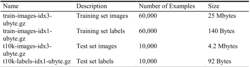
already includes the Fashion-MNIST as a built-in dataset. The total size of the Fashion-MNIST dataset is approximately 29.2002 megabytes. Table 1 provides a full breakdown of file sizes for training and test sets [19].
Table 1. Files Contained in the Fashion-MNIST Dataset.
Name Description Number of Examples Size
train-images-idx3-ubyte.gz
Training set images 60,000 25 Mbytes
train-images-idx1-ubyte.gz
Training set labels 60,000 140 Bytes
t10k-images-idx3-ubyte.gz
Test set images 10,000 4.2 Mbytes t10k-labels-idx1-ubyte.gz Test set labels 10,000 92 Bytes
TensorFlow is one of such APIs that contains the Fashion-MNIST dataset, and is employed in our work for building CNNs. Fashion-MNIST is a dataset comprised of
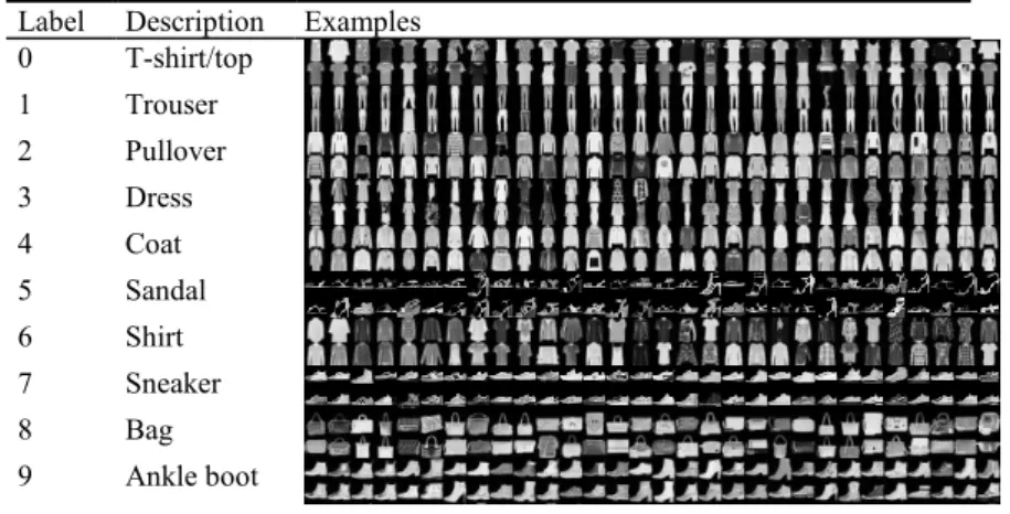
article images from Zalando, Europe’s leading online platform for fashion [19], [20]. Each observation contained in the dataset is a greyscale image by the size of 28 by 28 pixels [19]. Moreover, each observation is tagged with one of ten classification labels [19]. Table 2 reflects the potential labels an observation can have [19]. The default training and test sizes are 60,000 and 10,000 observations, respectively [19].
Table 2. Label Classification of Clothing. Label Description Examples 0 T-shirt/top 1 Trouser 2 Pullover 3 Dress 4 Coat 5 Sandal 6 Shirt 7 Sneaker 8 Bag 9 Ankle boot
4.3 Fashion-MNIST Data Preprocessing
Rasul and Xiao have preprocessed the Fashion-MNIST dataset with regards to data cleansing [19]. TensorFlow shuffles the data as a preprocessing step before importation. Consequently, training the model on batches of highly correlated observations is avoided. However, some data munging is still required.
The greyscale values contained in the x_train and x_test sets are of the type uint8. These values are converted to a type of float32 and then dimensionally normalized so that both are of the same scale [21]. Then a subset of the training set is partitioned for the purposes of validation. In particular, 5,000 observations are removed from the x and y training sets and assigned to the new x and y validation sets. Table 3 displays the number of observations in each set with the inclusion of the validation set [21].
Table 3. Total Number of Observation per Dataset.
Name Description Number of Observations Training set Used for model training 55,000
Validation set Used for tuning hyperparameters 5,000 Test set Used for model testing after
validation 10,000
In order to be compatible with the Keras Sequential Model API, all three sets of data pertaining to the greyscale values are reshaped from the dimension of “(28, 28)” to a dimension of “(28, 28, 1)” [21]. The data is now ready for model building and metric evaluation.
5 Convolutional Neural Network Results
5.1 Hyperparameter Tuning
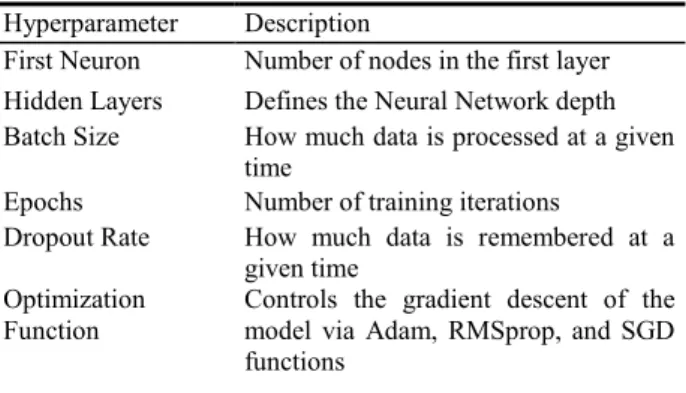
Before testing the impact of training data size on the validation accuracy of a CNN, the hyperparameters need to be decided upon. 648 models, each with their own distinct set of hyperparameters were trained and tested on the Fashion-MNIST dataset. The purpose of testing this large swath of models was to discern an optimal set hyperparameters with which to statistically test the impact of training data size on validation accuracy. Table 4 reflects the six hyperparameters that were tuned via training and testing the 648 CNNs.
Table 4. Hyperparameter Tuning for CNNs. Hyperparameter Description
First Neuron Number of nodes in the first layer Hidden Layers Defines the Neural Network depth Batch Size How much data is processed at a given
time
Epochs Number of training iterations
Dropout Rate How much data is remembered at a given time
Optimization
Function Controls the gradient descent of the model via Adam, RMSprop, and SGD functions
5.2 Distribution of Model Performance
The kernel density plot displayed in Figure 4 reflects the distribution of model performance based on validation accuracy. The red circles highlight the four underlying subpopulations that exist within our models. These subpopulations are neighborhoods of models with similar hyperparameters.
Fig. 4. Distribution of Model Performance Based on Validation Accuracy.
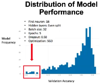
The histogram displayed in Figure 5 sheds light on the worst performing modal point. Within this neighborhood of models, the most common hyperparameters were found to be: A first neuron of 16 nodes, an even split of hidden layers, a batch size of 32, 5 epochs, a dropout rate of 0.50, and an optimization function of SGD.
Fig. 5. Worst Performing Modal Point Based on Validation Accuracy.
The histogram displayed in Figure 6 sheds light on the second worst performing modal point. Within this neighborhood of models, the most common hyperparameters were found to be: A first neuron of 32 nodes, an even split of hidden layers, a batch size of 32, 5 epochs, a dropout rate of 0.50, and an optimization function of SGD.
Fig. 6. Second Worst Modal Point Based on Validation Accuracy.
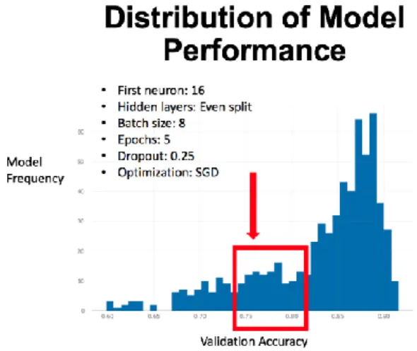
The histogram displayed in Figure 7 sheds light on the second best performing modal point. Within this neighborhood of models, the most common hyperparameters were found to be: A first neuron of 16 nodes, an even split of hidden layers, a batch size of 8, 5 epochs, a dropout rate of 0.25, and an optimization function of SGD.
Fig. 7. Second Best Modal Point Based on Validation Accuracy.
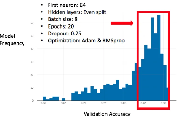
The histogram displayed in Figure 8 sheds light on the best performing modal point. Within this neighborhood of models, the most common hyperparameters were found to be: A first neuron of 64 nodes, an even split of hidden layers, a batch size of 8, 20 epochs, a dropout rate of 0.25, and a roughly even split between Adam and RMSprop for optimization function.
Fig. 8. Best Modal Point Based on Validation Accuracy.
5.3 Hyperparameter Selection of Top Performing Models
The most common hyperparameters from the top 10 performing models, based on validation accuracy, are chosen as an optimal set of hyperparameters with which to test the training size impact on validation accuracy. In particular, the set of hyperparameters to be used are as follows: A first neuron size of 64 nodes, 1 hidden layer, a batch size of 8, 20 epochs, a dropout rate of 0.25, and the Adam optimization function. Figure 9 compares the location of the top ten performing models against the distribution of the rest of the models.
Fig. 9. Top Ten Performing Models by Validation Accuracy.
5.4 Validation Accuracy of Varying Training Set Sizes
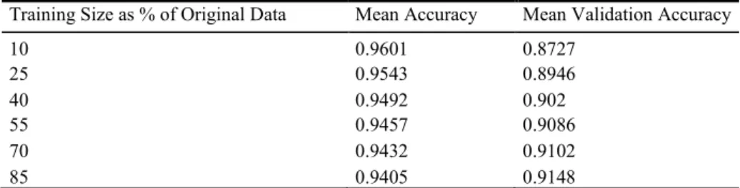
After an optimal set of hyperparameters were found, the CNN was trained on varying sizes of the original dataset. Specifically, the training set sizes range from 51,000 down to 6,000 by increments of 9,000. The CNN was trained on each of these six varying training sizes ten times. The group means of accuracy and validation accuracy for each of the training set sizes are reflected in Table 5.
Table 5. Mean Accuracies by Training Set Size.
Training Size as % of Original Data Mean Accuracy Mean Validation Accuracy
10 0.9601 0.8727 25 0.9543 0.8946 40 0.9492 0.902 55 0.9457 0.9086 70 0.9432 0.9102 85 0.9405 0.9148
6 Convolutional Neural Network Analysis
6.1 One-Way Analysis of Variance for Validation Accuracy
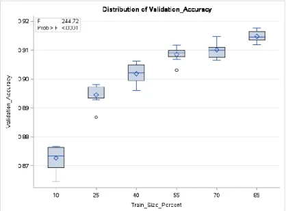
A one-way analysis of variance (ANOVA) considers one treatment factor with two or more treatment levels [22]. The goal of this analysis is to test for differences among the means of the levels and to quantify these differences [22]. The null hypothesis of this test is that the mean validation accuracies of all training set sizes are equal. In contrast, the alternative hypothesis is that not all of the mean validation accuracies of all the training set sizes are equal. Figure 10 displays the one-way analysis of validation accuracy variance conducted upon the differing training set sizes.
Fig. 10. Top Ten Performing Models by Validation Accuracy.
Visually, the boxplots reflect a decreasing rate of return with regards to validation accuracy as the training set size increases. Moreover, there is no quantile overlap between using 10% versus 25% of the original data as training sets. Furthermore, a validation accuracy of 90% is achieved by using only 40% of our original data as a training set. We can confirm this via the p-value of our statistical test. The p-value for this ANOVA test is less than 0.0001. At an alpha level of 0.05, this p-value is highly statistically significant. Since the p-value is less than the alpha level, we reject our null hypothesis. In other words, there is evidence to suggest that training size has an effect on validation accuracy for a CNN. By randomly selecting our observations during the stratified split, we can we can infer training set sizes caused differences in
validation accuracies. However, we cannot infer that training set sizes cause differences in validation accuracies for other algorithms.
7 Ethical Issues of Classification
On the surface level, there is no ethical issue with identifying articles of clothing and classifying them correctly. However, the over-arching scheme of object classification lends itself to possible ethical issues.
For example, China’s social credit system is fueling research and development into
technologies that can track and identify an individual’s face, gait, and even their
clothing [23]. These metrics help determine a Chinese citizen’s social credit score
[23]. Subsequently, a Chinese citizen’s social credit score affects their ability to
travel, internet speed, access to education, and even whether or not they are publicly shamed [23].
There is an ethical issue with determining someone’s social value and standing
based on how they dress. Because of the ability of classification algorithms to identify objects in the public space, and to glean intimate information about someone, the ethical duties of a data scientist are numerous.
According to the Association for Computing Machinery’s (ACM) code of ethics,
“technology enables the collection, monitoring, and exchange of personal information quickly, inexpensively, and often without the knowledge of the people affected” [24]. Because of this, the duties of anyone using technology in an impactful manner are to communicate what they are doing, how they are doing it, what the findings mean, and how the findings affect the user. These duties are not only of paramount importance but should be ever evolving and continuous.
In the ACM’s code of ethics, it states that anyone using technology in an impactful
manner “should only use personal information for legitimate ends and without violating the rights of individuals and groups” [24]. Additionally, people exercising
impactful technology “should establish transparent policies and procedures that allow individuals to understand what data is being collected and how it is being used, to give informed consent for automatic data collection, and to review, obtain, correct inaccuracies in, and delete their personal data” [24]. With this in mind, anyone fueling or conducting research and development into technologies that perform object classification on individuals, whether it be their face or clothing, need to address
individuals’ expectations of privacy as to not violate them.
8 Conclusions
The number of hidden layers in the Convolutional Neural Network employed in this paper had no impact on validation accuracy. This assertion is supported by the roughly equivalent distribution of models containing one, two, and three hidden layers throughout the 4 modal points in the kernel density plot displayed in Figure 4. One would think the best performing models would contain more hidden layers, whereas
the worst performing models would contain fewer hidden layer, due to neural density playing an important role validation accuracy.
Of the hyperparameters tested, the first neuron, dropout, and optimization function had the greatest impact on validation accuracy. The best 10 models predominantly had 64 neurons, and a dropout rate of 0.25, which supports the notion that a denser neural network is more accurate. Furthermore, the SGD optimization function was only found in the bottom 3 modal points containing the worst performing models. Moreover, only ADAM and RMSprop were found in the best performing models. In addition, epoch training times of 20 were predominately found in the top preforming models suggesting more training iterations increase the validation accuracy.
Evidence suggests training size causes validation accuracy. Without at least 40% of our original training data, or 24,000 samples, we were not able to achieve a 90% validation accuracy. Moreover, there is a diminishing rate of return on validation accuracy as the training sizes increase. This makes sense because you cannot have an accuracy greater than 100%, so it is in essence the upper bound.
References
1. Jordan, M I, and T M Mitchell. “Machine Learning: Trends, Perspectives, and Prospects.”
Science (New York, N.Y.), vol. 349, no. 6245, 2015, p. 255., doi:10.1126/science.aaa8415
2. Ghosh, Biplab. “10 Amazing way Deep Learning will rule the world in 2018 and beyond.”
20, Aug 2017. KnowStartup.com. Accessed 07 Nov 2018.
Http://knowstartup.com/2017/08/10-amazing-ways-deep-learning-will-rule/
3. Martín Abadi, Ashish Agarwal, Paul Barham, Eugene Brevdo, Zhifeng Chen, Craig Citro, Greg S. Corrado, Andy Davis, Jeffrey Dean, Matthieu Devin, Sanjay Ghemawat, Ian Goodfellow, Andrew Harp, Geoffrey Irving, Michael Isard, Rafal Jozefowicz, Yangqing Jia, Lukasz Kaiser, Manjunath Kudlur, Josh Levenberg, Dan Mané, Mike Schuster, Rajat Monga, Sherry Moore, Derek Murray, Chris Olah, Jonathon Shlens, Benoit Steiner, Ilya Sutskever, Kunal Talwar, Paul Tucker, Vincent Vanhoucke, Vijay Vasudevan, Fernanda Viégas, Oriol Vinyals, Pete Warden, Martin Wattenberg, Martin Wicke, Yuan Yu, and Xiaoqiang Zheng. TensorFlow: Large-scale machine learning on heterogeneous systems, 2015. Software available from tensorflow.org. Accessed 08 July 2018
Https://www.tensorflow.org/api_docs/python/tf/keras/datasets/fashion_mnist/load_data
4. Ng, Andrews. “The State of Artificial Intelligence.” MIT Technology Review. 15 Dec 2017. Accessed 15 July 2018. Https://www.youtube.com/watch?v=NKpuX_yzdYs
5. Goodfellow, Ian. “Instead of moving on to harder datasets than MNIST, the ML Community is studying it more than ever. Even proportional to other datasets.” Twitter. 13 Apr 2017. Accessed 08 July 2018
6. Rasul, Kashif, Xiao, Han. “Fashion-MNIST.” Zalando Research. Accessed 08 July 2018.
Https://research.zalando.com/welcome/mission/research-projects/fashion-mnist/ 7. Roberts, Eric. “Neural Networks History: The 1940’s to the 1970’s.” Stanford University,
Department of Computer Science. Accessed 09 July 2018.
Https://cs.stanford.edu/people/eroberts/courses/soco/projects/neural-networks/History/history1.html
8. Roberts, Eric. “Neural Networks History: The 1980’s to thePresent.” Stanford University,
Department of Computer Science. Accessed 09 July 2018.
Https://cs.stanford.edu/people/eroberts/courses/soco/projects/neural-networks/History/history2.html
9. Hochreiter, Sepp, Schmidhuber, Jürgen. “Long Short-Term Memory.” Institute of
Bioinformatics, Johannes Kepler University. Neural Computation, volume 9, pp. 1735-1780, 1997. Accessed 10 July 2018. Http://www.bioinf.jku.at/publications/older/2604.pdf/ 10. “A Collection of Neural Network Use Cases and Applications.” Pressive. 06 Aug 2017.
Accessed 09 July 2018. Http://analyticscosm.com/a-collection-of-neural-network-use-cases-and-applications/
11. Karpathy, Andrej. “CS231n Convolutional Neural Networks for Visual Recognition.”
Stanford University. Access 09 July 2018. Https://cs231n.github.io/convolutional-networks/#conv
11. Patrice Y. Simard, Dave Steinkraus, John C. Platt Microsoft Research. “Best Practices for
Convolutional Neural Networks Applied to Visual Document Analysis.” Microsoft, 01 Aug
2003. Accessed 10 July 2018. Https://www.microsoft.com/en-us/research/wp-content/uploads/2003/08/icdar03.pdf
12. Chollet, Fraçois, and others. “Keras,” 2015. Accessed 09 July 2018. Https://keras.io/ 13. Nitish Srivastava, Geoffrey Hinton, Alex Krizhevsky, Ilya Sutskever, Ruslan
Salakhutdinov. “Dropout: A Simple Way to Prevent Neural Networks from Overfitting.”
Journal of Machine Learning Research, Volume 15, 2014, pp. 1929-1958. Accessed 09 July 2018.
Http://www.jmlr.org/papers/volume15/srivastava14a/srivastava14a.pdf?utm_content=buffer 79b43&utm_medium=social&utm_source=twitter.com&utm_campaign=buffer
14. LeCun, Yann, Cortes, Corinna, and J.C. Burges, Christopher. “The MNIST Database.” The
Courant Institute of Mathematical Sciences, New York University. Accessed 08 July 2018. Http://yann.lecun.com/exdb/mnist/
15. Robinson, David. “mnist_pairs.R,” GithubGist, 31 May 2017. Accessed 08 July 2018. Https://gist.github.com/dgrtwo/aaef94ecc6a60cd50322c0054cc04478
16. Taus Priyo, Shehzad Noor. “Image Classification Using Deep Learning: “Hello World” Tutorial.” Medium. 06 Mar 2017. Accessed 08 July 2018.
Https://medium.com/@sntaus/image-classification-using-deep-learning-hello-world-tutorial-a47d02fd9db1
17. Hamner, Ben. “Popular Dataset References Over Time.” Kaggle. 05 Dec 2016. Accessed 08 July 2018. Https://twitter.com/benhamner/status/805864969065689088
18. Chollet, Fraçois. “Many good ideas will not work well on MNIST (e.g. batch norm). Inversely many bad ideas may work on MNIST and no transfer to real CV.” Twitter. 13 Apr 2017. Accessed 08 July 2018. Https://twitter.com/fchollet/status/852594987527045120 19. Xiao, Han, Rsul, Kashif, Vollgraf, Roland. “Fashion - MNIST: a Novel Image Dataset for
Benchmarking Machine Learning Algorithms.” 25 Aug 2017. Accessed 08 July 2018. Https://arxiv.org/abs/1708.07747v2
20. Zalando Research. “Big Ideas Call for a Platform to Match.” Accessed 08 July 2018. Https://jobs.zalando.com/en/about/
21. Maynard-Reid, Margaret. “Fashion-MNIST with tf.Keras.” 24 Apr 2018, Medium.
Accessed 08 July 2018. Https://medium.com/tensorflow/hello-deep-learning-fashion-mnist-with-keras-50fcff8cd74a
22. SAS Institute Inc. 2008. SAS/STAT®9.2 User’s Guide. Cary, NC: SAS Institute Inc
23. Mozur, Paul. “Inside China’s Dystopian Dreams: A.I., Shame and Lots of Cameras.” The New York Times, 08 July 2018. Accessed 02 Nov 2018.
Https://www.nytimes.com/2018/07/08/business/china-surveillance-technology.html 24. Gotterbarn, Don, Brinkman, Bo, Flick, Catherine, Kirkpatrick, Michael S., Miller, Keith,
Varansky, Kate, Wolf, Marty J., “ACM Code of Ethics and Professional Conduct.”
Association for Computing Machinery, 22 June 2018. Accessed 13 Sept 2018. Https://www.acm.org/code-of-ethics