Construct validation of a DCM for resting state fMRI

(1)

Technical Note

Construct validation of a DCM for resting state fMRI

Adeel Razi

a,b,

⁎

_{, Joshua Kahan}

c

_{, Geraint Rees}

a,d

_{, Karl J. Friston}

a a

The Wellcome Trust Centre for Neuroimaging, University College London, 12 Queen Square, London WC1N 3BG, UK b

Department of Electronic Engineering, NED University of Engineering and Technology, Karachi, Pakistan

c_{Sobell Department of Motor Neuroscience & Movement Disorders, Institute of Neurology, University College London, Queen Square, London, WC1N 3BG, UK} d

Institute of Cognitive Neuroscience, University College London, 17 Queen Square, London WC1N 3AR, UK

a b s t r a c t

a r t i c l e i n f o

Article history:

Accepted 13 November 2014 Available online 21 November 2014 Keywords:

Dynamic causal modelling Effective connectivity Functional connectivity Resting state fMRI Graph Bayesian Network discovery

Recently, there has been a lot of interest in characterising the connectivity of resting state brain networks. Most of the literature uses functional connectivity to examine these intrinsic brain networks. Functional connectivity has well documented limitations because of its inherent inability to identify causal interactions. Dynamic causal modelling (DCM) is a framework that allows for the identification of the causal (directed) connections among neuronal systems—known as effective connectivity. This technical note addresses the validity of a recently proposed DCM for resting state fMRI–as measured in terms of their complex cross spectral density–referred to as spectral DCM. Spectral DCM differs from (the alternative) stochastic DCM by parameterising neuronalfl uctu-ations using scale free (i.e., power law) forms, rendering the stochastic model of neuronal activity deterministic. Spectral DCM not only furnishes an efficient estimation of model parameters but also enables the detection of group differences in effective connectivity, the form and amplitude of the neuronalfluctuations or both. We com-pare and contrast spectral and stochastic DCM models with endogenousfluctuations or state noise on hidden states. We used simulated data tofirst establish the face validity of both schemes and show that they can recover the model (and its parameters) that generated the data. We then used Monte Carlo simulations to assess the accuracy of both schemes in terms of their root mean square error. We also simulated group differences and com-pared the ability of spectral and stochastic DCMs to identify these differences. We show that spectral DCM was not only more accurate but also more sensitive to group differences. Finally, we performed a comparative evaluation using real resting state fMRI data (from an open access resource) to study the functional integration withindefault mode networkusing spectral and stochastic DCMs.

Introduction

In recent years there has been a marked increase in research that

com-bines resting state fMRI with large-scale‘network analyses’(Nakagawa

et al., 2013; Smith et al., 2013; Wang et al., 2010). The majority of studies

report functional connectivity, reﬂecting statistical dependencies

(e.g. temporal correlations) between spatially remote neurophysiological regions. These correlations are inherently undirected, and preclude infer-ence about (directed) causal interactions among neuronal systems. In

contrast, effective connectivity summarises the causal inﬂuence one

neural system exerts over another using a model of neural interactions that best explains the observed signals or their functional connectivity: in brief, effective connectivity causes functional connectivity. Effective connectivity is, necessarily, directed. However, it should be noted that functional connectivity can also be directed; e.g., partial correlation and parametric (resp. nonparametric) Granger causality based on

Yule–Walker (resp. Wilson–Burg) formulations. These characterisations

provide measures of directed statistical dependencies because they con-sider how much past observations predict the current observation (Friston et al., 2014a).

We recently introduced a new dynamic causal model (DCM) for

modelling intrinsic dynamics of a resting state network (Friston et al.,

2014b). This DCM estimates the effective connectivity among coupled populations of neurons, which subtends the observed functional con-nectivity in the frequency domain. We refer to this as spectral DCM (spDCM). Spectral DCM uses a neuronally plausible power-law model of the coupled dynamics of neuronal populations to generate complex cross spectra among measured responses. In particular, this spectral

DCM is distinct from stochastic DCM (sDCM) (Friston et al., 2011; Li

et al., 2011) as it eschews the estimation of randomﬂuctuations in (hidden) neural states; rendering spectral DCM essentially deterministic in nature.

In this paper, we establish the construct validity of spectral DCM by comparing and contrasting it with stochastic DCM. This paper comprises of four sections. We begin by rehearsing the theoretical background of both spectral and stochastic dynamic causal models. ⁎ Corresponding author at: The Wellcome Trust Centre for Neuroimaging, Institute of

Neurology, UCL, Queen Square, London WC1N 3BG, UK. E-mail address:[email protected](A. Razi).

http://dx.doi.org/10.1016/j.neuroimage.2014.11.027

NeuroImage

(2)

These models are similar to conventional deterministic DCM for fMRI (Friston et al., 2003) but include these statistics of endogenous activity

that reproduce functional connectivity (correlations)_—of the sort

ob-served in resting state fMRI. DCMs for resting state data are also slightly simpler: given that most resting state designs compare groups of sub-jects (e.g. patient cohorts vs. controls); spDCMs do not usually require

the bilinear term (accounting for condition-speciﬁc effects on effective

connection strengths). In the second section, we address construct validation of spectral DCM against stochastic DCM, using simulated time series. We compare the accuracy of model inversion, demonstrating

that‘true’effective connectivity can be recovered using both schemes

with an acceptable root mean square error. In the third section, we repeat the simulations but with simulated group differences, to see if the schemes can successfully recover true differences in effective connec-tivity. In the fourth section, we conclude with an empirical (compara-tive) evaluation using data available from an open source database, with an illustrative focus on functional integration within the default mode network.

Dynamic casual modelling of resting brain networks

There has been a large surge of research recently examining

sponta-neousﬂuctuations in Blood Oxygen Level Dependent (BOLD) fMRI signals

measured using fMRI. Theseﬂuctuations can be attributed to the

sponta-neous neural activity, which is usually ignored in the deterministic DCM models of responses to (designed) experimental inputs.

Classically, deterministic DCMs are cast as multiple input multiple output (MIMO) systems, where the experimentally designed inputs enter the brain to produce an observed BOLD response. In the absence

of external inputs–as is the case in the resting state fMRI–one would

imagine that neuronal networks are perturbed by activity that is internal

to the system or by intrinsic_ﬂuctuations seen in any biological system for

e.g. seeFaisal et al. (2008). These perturbations are the endogenous

neu-ralﬂuctuations, which are responsible for driving the coupled dynamics

of the hidden neuronal states. The inclusion of the neuralﬂuctuations

means that the model is now based on random differential equations having both the drift and diffusion components. The drift component of this random differential equation entails the Jacobian; i.e., the effective connectivity matrix, whilst the diffusion component models the

endoge-nousﬂuctuations. We have introduced several schemes that can invert

these sorts of models (Friston et al., 2010, 2014b; Li et al., 2011) that differ

according to how the endogenousﬂuctuations are treated.

Model inversion using sDCM estimates both the effective connectivity

and the neuronalﬂuctuations from the BOLD signal, which entails a difﬁ

-cult triple estimation problem and uses advance methods likegeneralised

ﬁltering(Friston et al., 2010) for parameter estimation. In contrast,

spDCM parameterises the form of the endogenousﬂuctuations; speciﬁ

-cally, by characterising them in terms of their cross spectral densities.

This eliminates the need to estimate the neuronalﬂuctuations and

signif-icantly simplifying model inversion. In what follows, we brieﬂy review

these models in turn. It is useful to remember that DCM for fMRI consists of two parts; (1) the neuronal state model, describing how the dynamics of coupled neuronal populations interact, and (2) the haemodynamic model, which transforms hidden neural states of each population or

region into predicted BOLD responses—using a previously established

biophysical model (Buxton et al., 1998; Friston et al., 2003; Stephan

et al., 2007). In this paper, we are only concerned with theﬁrst (neuronal)

part, without changing the second (haemodynamic) part: seeStephan

et al. (2007).

The generative model

In modelling resting state activity, it is necessary to augment the ordinary differential equations used in standard DCM, with a stochastic

term to model endogenous neuronalﬂuctuations. This renders the

equations of the motion stochastic. Stochastic equations are most

frequently used to model the behaviour of (open) systems operating

near or far from equilibrium that are perturbed byﬂuctuations in the

(thermal) environment. The stochastic generative model for the resting state fMRI time series, like any other DCM, comprises of two equations: the Langevin form of evolution equation (motion) is written as:

x

t

ð Þ ¼f x tðð Þ;u tð Þ;θÞ þ v tð Þ; ð1Þ

and the observation equation, which is a static nonlinear mapping from

the hidden physiological states1_in₍₁₎_{to the observed BOLD activity}

and is written as:

y tð Þ ¼h x tð ð Þ;φÞ þ e tð Þ; ð2Þ

whereẋ(t) is the rate in change of the neuronal statesx(t),θare

un-known parameters (i.e. the effective connectivity) andv(t) (resp.e(t))

is the stochastic process–called the state noise (resp. the measurement

or observation noise)–modelling the random neuronalﬂuctuations

that drive the resting state activity. In the observation equations,φare

the unknown parameters of the (haemodynamic) observation function

andu(t) represents any exogenous (or experimental) inputs that drive

the hidden states—that are usually absent in resting state designs. Here,

we will assume a generalised framework in whichv(t) ande(t) are

ana-lytic (i.e., non-Markovian). This simply means thatgeneralisedmotion of

the state noiseev tð Þ ¼v tð Þ;vð Þt;€v tð Þ…is well deﬁned in terms of its co-variance. Similarly, the observation noise (t) = [e(t),ė(t),ë(t)…] has

well deﬁned covariance (for a more detailed discussion seeFriston,

2008). Consequently, the diffusion part of the generative model above

can be conveniently parameterised in terms of its precision (inverse

covariance). This allows us to cast(1)as random differential equation

in-stead of stochastic differential equation hence eschewing Ito calculus (Friston et al., 2010; Li et al., 2011).

Statistical assumptions about the higher order motion of generalised state noise implicitly specify its degree of smoothness. Interested

readers willﬁnd a theoretical motivation for using analytic state noise

in the context of studying brain dynamics in (Friston et al., 2010).

Note that standard stochastic differential equations (and related Ito

cal-culus) rely upon theﬂuctuations being a mixture of Wiener processes,

which are non-differentiable functions of time (Kloeden and Platen,

1999). This corresponds to a special case of generalised state noise

whose high order motion has inﬁnitely high prior variance (unbounded

roughness). Within the above class of generalised state-space models, standard Markovian state-space models are thus rather special (and biologically implausible) cases of generalised models.

Under linearity assumptions, Eqs.(1) and (2)can be written

com-pactly in generalised coordinates of motion:

Dex tð Þ ¼efðex;eu;θÞ þev tð Þ; ð3Þ ey tð Þ ¼ehðex;φÞ þ ee tð Þ; ð4Þ

whereDis the block diagonal temporal derivative operator, such that

the vectors of generalised coordinates of motion are shifted as we move from lower-orders of motion to higher-orders. This means that

theﬁrst leading diagonal ofDcontains identity matrices. For a more

de-tailed derivation and explanation please seeFriston (2008). For resting

state activity, Eq.(3)takes on a very simple linear form:

Dex tð Þ ¼Aex tð Þ þCeu tð Þ þev tð Þ; ð5Þ

whereAis the Jacobian describing the behaviour–i.e. the effective

connectivity_–of the system near its stationary point (f(xo) = 0) in

the absence of theﬂuctuationsṽ(t). Eq.(5)is an instance of a linear

dynamical system and has quasi-deterministic behaviour (Daunizeau

1

Strictly speaking, the hidden states include both neuronal and haemodynamic states; however, for simplicity, we will ignore haemodynamic states in this paper.

(3)

et al., 2012; Tropper, 1977). Put simply, the linear dynamical system

described by Eq.(5)is insensitive to the initial conditions; hence, it

can only exhibit a limited repertoire of behaviour: linear systems

can contain closed orbits, but they will not beisolated, hence no

limit cycles–either stable or unstable–can exist, which precludes

chaotic behaviour. Technically speaking, if_λrepresents the eigenvalues

of the Jacobian∂_exf ¼A, that isλ=ν

†_A_ν_{, where}_†_{denotes the}

general-ised inverse, then the Lyapunov exponentsℜ(λ) of this linear dynamical

system will always be negative. In general, the Jacobian is not symmet-rical (causal effects are asymmetric); hence the modes and eigenvalues take complex values. For the detailed treatment of the special case of

symmetrical connectivity–in which the eigenmodes of functional and

effective connectivity become the same–seeFriston et al. (2014c).

The real part of the eigenvalues plays the role of Lyapunov exponents, whereas the imaginary part represents the oscillatory portion of the response, which will decay (or grow) with the real part. In terms of dynamical behaviour, irrespective of the amount of the stochastic noise, the average trajectory of the stochastic system would follow the

trajectory of its deterministic variant_—in the absence of any stochastic

forcing term.

Dynamic instabilities and intrinsic brain networks

Although the resting state model of effective connectivity is simple–

and admits only a limited repertoire of dynamical behaviour–the

inclu-sion of endogenousﬂuctuations provides a plausible model of intrinsic

brain networks: intrinsic dynamics are thought to be generated by the

dynamic instabilities that occur nearbifurcations; i.e., dynamics that

accompany a loss of stability when certain control parameter(s) reach a

critical value (Deco and Jirsa, 2012; Freyer et al., 2011; Robinson et al.,

2002). The eigenmodes of effective connectivity that deﬁne the stability

of the resting state give rise to scale-freeﬂuctuations that emerge from

the superposition of the few modes that decay slowly. These slowly

ﬂuctuating (unstable) modes have Lyapunov exponents that are close

to zero. This occurs when systems approachtranscriticalbifurcations

(or stochastic Hopf bifurcations) when the eigenvalues are complex

(Aburn et al., 2012; Robinson, 2003) and show critical slowing (Kelso,

2010). This simply means that the ensuing networks are deﬁned by

tra-jectories that have aﬁxed point that always exists but which is also

close to instability. This means that the neural_ﬂuctuations persist over

longer time scales to generate the patterns responsible for the emergence of intrinsic brain networks. The (negative) inverse of the Lyapunov expo-nent corresponds to the characteristic time constant of each mode, where each mode corresponds to an intrinsic brain network.

Free energy and Bayesian model inversion

Having considered DCMs of resting state activity, we turn to model inversion. Bayesian model inversion means that we infer the parameters of the model in Eqs.(3) and (4), from the observed signaly(t). Since this inversion is computationally exorbitant, requiring high-dimensional in-tegrals (either by brute force numerical methods or sampling schemes),

we resort to schemes based on approximatevariational Bayesian

infer-ence. Variational Bayes approximates the conditional posterior density

p(ψ|y,m)–of model parametersψwith datayfor a given modelm–by

a variational or proposal densityq(ψ). Importantly, this approximation

is optimised by maximising model log-evidence, which can be expressed mathematically as

lnp yð jmÞ ¼F yð;qÞ þDKL½qð Þjjψ pðψjy;mÞ; ð6Þ

whereF(y,q) is thefree energyandDKLis the Kullback–Leibler divergence.

In turn, free energy can be expressed as

F yð;qÞ ¼Eq lnpðψ;yjmÞ–Eq½lnqð Þψ

h i

;

¼Eq½lnp yð jψ;mÞ þ lnpðψjmÞ–Eq½lnqð Þψ;

ð7Þ

whereEq½ :is the expectation operator with respect toq(ψ). There are few

important observations to make here: Firstly, from Eq.(6)free energy

F(y,q)≤lnp(y|m) is always a lower bound on the model log evidence be-cause the divergence term is always positive and only becomes zero whenq(ψ) =p(ψ|y,m). Secondly, maximisingF(y,q) automatically

min-imizes the divergence term hence givingq(ψ)≈p(ψ|y,m). In other

words, by maximising negative free energy with respect to the variational

density we get two things;_ﬁrst, the free energy becomes a proxy for log

model evidence (necessary for model comparison) and second, the varia-tional density becomes posterior density over parameters (necessary for model identi_ﬁcation).

Under the Laplace assumption, the proposal density assumes a

Gaussian formqð Þ ¼ Nψ ðμ;ΣÞ, where the variational parameters,

μandΣ, corresponds to the conditional mean and covariance

respec-tively. The free energy from Eq.(7)–under Laplace approximation–

can now be written as

F yð ;qÞ ¼ lnp yð jμ;mÞ þ lnpðμjmÞ þ 1

2½lnjΣj þn ln 2πe; ð8Þ

wherenis the number of the parameters in the setψ.

Another assumption that simpliﬁes the maximisation of free energy

F(y,q) is the meanﬁeld assumption used in statistical physics. This

means that one can factorise the proposal density over a set of parameters such that

qð Þ ¼_ψ ∏iq ψ i

: ð9Þ

In other words,F(y,q) is maximised with respect toq(ψi_{) when there} is no variation in free energy with respect toq(_ψi_{) (}_{Friston et al., 2007}_). Mathematically this can be written as:

ΔF y ;q ψi _¼ 0⇔∂F y;q ψ i ∂q ψi ¼0⇒ q ψi ¼ 1 Zi expI q ψi ; ð10Þ

whereZiis a normalization constant andI(q(ψi)) is the variational energy. In summary, model inversion reduces to maximising the free energy in

Eq.(8)with respect to the mean (and covariance) of the proposal density

over each set of parameters. DCM generally uses a gradient ascent scheme, known as the Variational Laplace (VL).

Inversion of stochastic models in time domain

Inverting the stochastic DCM of the form given by Eq.(1)in the time

domain, which includes state noise, is rather complicated because such models require estimation of not only the model parameters (and any

hyperparameters that parameterise the randomﬂuctuations), but also

the hidden states, which become random (probabilistic) variables. Hence the unknown quantities to be estimated under a stochastic DCM areψ¼fex tð Þ;φ;θ;σg, whereσrefers to any hyperparameters

(precisions or inverse covariances) deﬁning the neuronalﬂuctuations.

In terms of temporal characteristics, the hidden states are time-variant, whereas the model parameters (and hyperparameters) are time-invariant. There are various variational schemes in literature that can in-vert such models, for example, dynamic expectation maximisation (DEM) (Friston et al., 2008) and generalisedﬁltering (GF) (Friston et al.,

2010). There is a subtle but important distinction between DEM and GF.

(4)

assumesqð Þ ¼ψ qðex tð ÞÞqð Þφqð Þθqð Þσ , whereas generalisedﬁltering, as the name suggest, is more general in a sense that it does not make this

assumption. Both schemes, however, assume a_ﬁxed form Gaussian

dis-tribution for the approximate conditional posterior densities (the Laplace

approximation). Generalisedﬁltering considers all unknown quantities

to be conditionally dependant variables i.e., qð Þ ¼_ψ qðex_;_φ_;_θ_;_σÞ, and furnishes time-dependent conditional densities for all the unknown

quantities. The time-invariantparameters and hyperparameters are cast

as time-variant with the prior constraint that their temporal variation is very small. This translates into a smooth gradient ascent on the free energy landscape. In brief, this online scheme assimilates log-evidence at each time point, in the form of the free energy bound and provides time-dependant conditional densities for all unknown quantities. This is in contrast to schemes, like DEM (or deterministic model inversion

using VL) with meanﬁeld approximations that assimilates all the data

before computing the free energy. The marginal conditional densities for the time-averaged parameters (and hyperparameters) from

general-isedﬁltering (GF) are calculated by using Bayesian parametric averaging

(BPA). This allows one to compare GF with other schemes like the deter-ministic model inversion employed in spDCM.

Inversion of stochastic models in spectral domain

Although the stochastic models in Eq.(1)and their inversion in time

domain provide a useful means to estimate effective connectivity they

also require us to estimate hidden states. This poses a difﬁcult inverse

problem that is computationally demanding; especially when the number

of hidden states becomes large. Toﬁnesse this problem, we recently

intro-duced a DCM based upon a deterministic model that generates predicted

cross spectra (Friston et al., 2014b). This scheme furnishes a constrained

inversion of the stochastic model by parameterising the neuronalﬂ

uctu-ations. This parameterisation also provides an opportunity to compare

parameters encoding the neuronalﬂuctuations among groups. The

parameterisation of endogenousﬂuctuations means that the states are

no longer probabilistic; hence the inversion scheme is signiﬁcantly

sim-pler, requiring estimation of only the parameters (and hyperparameters) of the model. The ensuing model inversion in the spectral domain is

similar in spirit to previous approaches described in (Freyer et al., 2012;

Robinson, 2003; Robinson et al., 2004). Put simply, whilst DEM or GF

estimates time-dependentﬂuctuations in neuronal states producing

ob-served fMRI data, spDCM simply estimates the time-invariant parameters of their cross spectra. Effectively, this is achieved by replacing the original time series with their second-order statistics (i.e., cross spectra), under stationarity assumptions. This means that, instead of estimating time varying hidden states, we are estimating their covariance, which does not change with time. This means that we need to estimate the covariance

of the randomﬂuctuations; where a scale free (power law) form for the

state noise (resp. observation noise) that can be motivated from previous

work on neuronal activity (Beggs and Plenz, 2003; Shin and Kim, 2006;

Stam and de Bruin, 2004):

gvðω;θÞ ¼αvω−βv geðω;θÞ ¼αeω−βv:

ð11Þ

Here, {α,β}⊂θare the parameters controlling the amplitudes and

exponents of the spectral density of the neuralﬂuctuations. This models

neuronal noise with generic1/fγspectra, which characterisesﬂ

uctua-tions in systems that are at nonequilibrium steady-state. A linear scaling

regime of the spectral density in double logarithmic coordinates–

implicit in(11)–is not by itself indicative of a scale free, critical process

unlessγis less than 1.5—and the regime scales over several orders of

magnitude. We note that for the human EEG, this is generally not the

case–above 10 Hz,γ= 2.5 and above 70 Hzγis usually greater than

3.5–which is consistent with a Poisson process (seeBedard et al.,

2006; Miller et al., 2009). At low frequencies (less than 1.5 Hz) the

slope is shallower and it is likely that the amplitude or power

enve-lopes of faster frequencies are scale-free (Kitzbichler et al., 2009;

Linkenkaer-Hansen et al., 2001) or heavy-tailed (Freyer et al., 2009). Using the model parameters,θL{A,C,α,β}, we can simply generate the expected cross spectra:

y tð Þ ¼κð Þt⊗v tð Þ þe tð Þ; κð Þ ¼t ∂xgexpðt∂xfÞ; gyðω;θÞ ¼jKð Þωj 2 gvðω;θÞ þgeðω;θÞ; ð12Þ

whereK(ω) is the Fourier transform of the system's (ﬁrst order)

Volterra kernelsκ(t), which are a function of the Jacobian or effective

connectivity. The unknown quantities_ψ= {_φ,_θ,_σ} of this deterministic

model can now be estimated using standard Variational Laplace

pro-cedures (Friston et al., 2007). The resulting inversion provides the

free energy bound on the log evidence lnp(gy(ω)|m) and approximate

conditional densitiesq(ψ)≈p(ψ|g(ω),m). Heregγ(ω) represents the

predicted cross spectra that can be estimated, for example, using

autoregressive (AR) model. Speciﬁcally, we use a fourth-order

auto-regressive model to ensure smooth sample cross spectra of the sort pre-dicted by the generative model. The frequencies usually considered for

fMRI range from 1

128 Hz to the Nyquist frequency (half the sampling

rate) in 32 evenly spaced frequency bins.

In summary, both sDCM and spDCM furnish estimates of the effective connectivity of endogenous brain networks from BOLD data acquired at rest, using different inversion schemes. We suppose that these resting state networks emerge from the dynamical instabilities and critical slowing near transcritical bifurcations. Hidden neuronal activity is modelled with random differential equations, which can be estimated

using stochastic inversion schemes (like generalisedﬁltering in sDCM),

or by deterministic scheme modelling observed functional connectivity

(speci_ﬁcally the cross spectral densities in the case of spDCM). In what

follows, we use Monte Carlo simulations to assess the performance of these schemes.

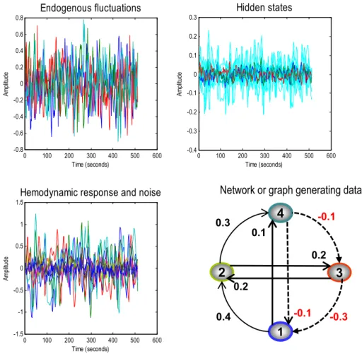
Comparative inversions and face validity

In this section, we address the face validity of the two schemes, com-paring the models based on deterministic and stochastic modelling of

neuronalﬂuctuations. Simulated time series were generated from a

four node graph (producing data over 512 time bins with a repetition

time of 2 s) with known effective connectivity (see Eq.(13) and

Fig. 1). Smooth neuronalﬂuctuations (resp. observation noise) driving each node were independently generated based on an AR(1) process

with an autoregressive coef_ﬁcient of one half, scaled to a standard

devi-ation of one fourth (resp. one eighth). The equdevi-ations of motion in

Eq.(1), together with haemodynamic observation Eq.(2)were used

to generate synthetic slow-varying time series, reminiscent of BOLD

data acquired at rest (Fig. 1). With these parameters, we produce a

maximum fMRI signal change of around 2%. The upper panels in

Fig. 1show the variations in the amplitude of endogenousﬂ uctua-tions that drive the changes in the hidden and haemodynamic states (cyan), which in turn produce the observed BOLD response. It is worth noting that the haemodynamic signal is much smoother than

the neuronal variations–that reﬂect the low-passﬁlter-like effect of

the haemodynamic transfer function–with a time constant of several

seconds.

To assess the face validity of both schemes, we used sDCM and spDCM to estimate the underlying effective connectivity of the same data. For this, we used the usual priors for the hidden states, parameters

(and hyperparameters) for stochastic DCM as described previously (Li

et al., 2011), as well as the same priors for {A,α,β} in spectral DCM as

described in (Friston et al., 2014b). The effective connectivity matrix

used for generating the simulations had four nodes with bottom-up (i.e. forward) and lateral connections having positive coupling, and the top-down edges having negative coupling (lower right panel of

(5)

Fig. 1). This architecture corresponds to the directed and cyclic connec-tivity matrix: A¼ −0:5 0 −0:3 −0:1 0:4 −0:5 0:2 0 0 0:2 −0:5 −0:1 0:1 0:3 0 −0:5 2 6 6 4 3 7 7 5: ð13Þ

Note that the equations of motion given by Eq.(5)—only yield critical

neuralﬂuctuations when the principal eigenvalues of the Jacobian (i.e.,A)

are close to zero (seeSpasojevic et al., 1996). The effective connectivity

matrix chosen here does not meet this criterion because of the strongly

damped self-connections—which are usuallyﬁxed (a priori) at−0.5

to preclude any run-away excitation.

The ensuing data we used to recover the known connection

strengths in Eq.(13)using the original time series (for stochastic

DCM) or their sample cross spectral density (for spectral DCM). The

pre-dicted and observed data features are presented inFig. 2. The sampled

(dashed lines) and predicted (solid lines) cross spectra of the data using spDCM were well matched. The upper left and right panels show the real and imaginary parts of the cross spectra respectively, whilst the second half of the upper left panel includes the cross covari-ance function (which is real in nature). The lower panel reports the

pre-dicted time series for each region (conditional expectations—solid lines)

and errors (red dashed lines) from the sDCM inversion. As previously

demonstrated (Li et al., 2011), the prediction error remained low,

generating a predicted time series that very much resembled the ob-served data.

The posterior estimates of the effective connectivity are shown in

Fig. 3. Posterior expectations are presented as grey bars with pink bars

indicating the 90% Bayesian conﬁdence intervals. We have also

superimposed the true connectivity as black bars for comparison. The upper left panel shows the posterior expectations for the spDCM inver-sion (shown as spectral in title), whilst the lower left panel shows the

results for the stochastic scheme using generalisedﬁltering. Clearly,

the spectral DCM's estimates are very accurate, with most of the extrinsic

connection strengths falling within 90% conﬁdence intervals. The

intrin-sic connections (i.e. the self-connections) are modelled as a (log) scale parameter and have a prior mean of zero. These connections are still es-timated with good accuracy showing around a 20% underestimation of the self-connectivity. The stochastic scheme also performed well, with estimates tending towards the true values but not as accurately as the deterministic (spectral) scheme. This reiterates the point that stochastic

DCM canﬁnd it difﬁcult to recover effective connectivity from data

gen-erated from graphs with reciprocal connectivity. We have also presented these results in a scatter plot to illustrate the relative accuracies of the spectral and stochastic estimates (the posterior estimates of spDCM are closer to the true parameters than those generated by the model based on sDCM). It can also be seen that the stochastic model underestimates

the parameters, a behaviour which has previously been reported (Li

et al., 2011) and is generally characteristic of approximate Bayesian in-ference schemes that contend with conditional dependencies.

0 100 200 300 400 500 600 -0.8 -0.6 -0.4 -0.2 0 0.2 0.4 0.6 0.8

Endogenous fluctuations

Time (seconds) Am pl itu de 0 100 200 300 400 500 600 -0.4 -0.3 -0.2 -0.1 0 0.1 0.2 0.3

Hidden states

Time (seconds) Am pl itu de 0 100 200 300 400 500 600 -1.5 -1 -0.5 0 0.5 1 1.5

Hemodynamic response and noise

Time (seconds)

A

m

pl

itude

Network or graph generating data

4

3

2 -0.1

1 -0.3

0.3

0.4

0.2

0.1 -0.1

Fig. 1.Thisfigure summarises the results of simulating fMRI responses to endogenousfluctuations over 512 time points (scans) with a TR of 2 s—here we only show initial 256 time bins. The simulation was based upon a simple four-region hierarchical network or graph, shown on the lower right, with positive effective connectivity (black) in the forward or ascending direction (and lateral direction) and negative (red) in the backward or descending direction. The four regions were driven by endogenousfluctuations (upper right panel) generated from an AR(1) process with autoregressive coefficient of one half (and scaled to a standard deviation of one quarter). Thesefluctuations caused distributed perturbations in neuronal states and consequent changes in haemodynamic states (shown as cyan) in the upper right panel, which produce thefinal fMRI response in the lower left panel.

(6)

Estimation accuracy and session length

In this section, we examine the accuracy of the estimates from the two DCMs as a function of the number of time bins sampled. It has previously been shown that including neural state noise yields more

accurate estimates for sDCM compared to its deterministic version–

which was extended to account for neuralﬂuctuations by projecting

the state noise to some temporal basis functions–especially so in the

presence of nonlinearities (Daunizeau et al., 2012). The spectral DCM

dif-fers from earlier deterministic formulations; here we are parameterising the neuronal state noise in frequency domain meaning, in principle, we are still using the same stochastic model but now the model inversion

uses second order data statistics—like their cross spectra.

When assessing the accuracy of the spectral and stochastic versions, we were primarily interested in establishing whether both versions can predict network parameters with an acceptable accuracy, whilst acknowledging their respective differences. The accuracy of sDCM has

been assessed previously (Daunizeau et al., 2012; Li et al., 2011). Here

the objective is to compare and contrast the accuracy of stochastic and spectral schemes. For this purpose we use the statistical measure of root mean squared error:

RMS_θ¼ ffiffiffiffiffiffiffiffiffiffiffiffiffiffiffiffiffiffiffiffiffiffiffiffiffiffiffiffiffiffiffiffiffiffiffiffiffiffiffiffi 1 n_θ X j¼1 n_θ θj−^θj 2 s ; ð14Þ

whereθand^θare the true and estimated parameter vectors respectively,

andnθis the length of these vectors. As argued inDaunizeau et al. (2012), the (root) mean squared error is an optimal measure of estimation

accuracy—in terms of Bayesian decision theory.

In Monte-Carlo simulations, we generated the time series of various lengths ranging from 128 time points to 1024 time points with a step

size of 128. We simulated 32 realisations (as a proxy for number of participants) for each run length and calculated the root mean squared error. The mean RMS error for each run length (averaging over 32

sim-ulations for each run length) is presented inFig. 4. For spDCM, RMS

error decreases as the number of time points increases. It is satisfying to note that the RMS drops below the typical effective connectivity value of 0.1 Hz, for times series with 384 time points, corresponding to around 13 min of scanning (with a repetition time of 2 s). Whilst the sDCM RMS also decreases with longer time series, the errors for sDCM estimates are greater than those for spDCM, and fail to reach the 0.1 Hz threshold. Whilst the accuracies of the sDCM estimates are impressive, demonstrating the scheme insensitivity to the run length, the estimation accuracy (for this particular graph) was inferior to spDCM. The Bayesian parameter averages (ignoring posterior

correla-tions) of the effective connectivity are shown inFig. 5as a function of

session length. As has been previously noted (Friston et al., 2014),

these Bayesian parametric averages do not change greatly when com-paring, for example, run lengths of 256 and 1024. As we are pooling

over many simulations, the conﬁdence intervals around these Bayesian

parameter averages are fairly small. This suggests that when a sufﬁcient

number of participants are used, shorter run lengths may provide rea-sonably accurate estimates.

In summary, on the basis of the simulations reported here (and many others not shown) it appears that spectral DCM outperforms

sto-chastic DCM in terms of accuracy—as measured by deviation from the

true parameters generating data. Having said this, the main difference between the two schemes is a greater shrinkage of Bayesian estimators for the stochastic scheme, which is consistent with the conditional de-pendencies between hidden states and parameters it has to contend with. In terms of construct validation, it is reassuring that both schemes

provide qualitatively similar (internally consistent) estimates—and

that both are consistent with the parameters of process generating data.

100 200 300 400 500 -2 -1.5 -1 -0.5 0 0.5 1 1.5

prediction and error (stochastic)

time

0 20 40 60 80 100 -0.2 0 0.2 0.4 0.6

Frequency and time (bins)

real

prediction and response (spectral)

0 20 40 60 80 100 -0.2 -0.1 0 0.1 0.2

Frequency and time (bins)

im

ag

ina

ry

prediction and response (spectral)

Fig. 2.Thisfigure reports the results of Bayesian model inversion using data shown in the previousfigure. This inversion produced predictions (solid lines) of sample cross spectra (dashed lines) and cross covariance functions, shown in the upper two panels for spectral DCM. The real values are shown on the left and the imaginary values on the right. Imaginary values are produced only by extrinsic (between regions) connections. Thefirst half of these responses and predictions correspond to the cross spectra between all pairs of regions, whilst the second half are the equivalent cross covariance functions—note that cross covariance only has real part. The lower panel shows the predicted response, in time, for the four regions and the associated error between the predictions and the observed responses.

(7)

Although being able to estimate effective connectivity from resting state fMRI may be interesting in and of itself, the usual questions in the setting are about differences in effective connectivity among cohorts, which we now look at more closely.

Comparative inversions testing for group differences

In this section, we examine whether group differences in effective connectivity can be detected by the two schemes. Group differences were simulated in the following way: Time series of 512 time points were generated for 48 participants using the above 4 node DCM (with

16 connections in total). Theﬁrst 24 instances used the connectivity

matrix given by(13), whilst the second 24 simulations were generated

using an altered matrix_—the strength of the extrinsic coupling from

node 2 to node 3 was made more excitatory (increased from 0.2 to 0.5 Hz). It should be noted that by making this connection stronger, we also break the symmetry in reciprocal connectivity between nodes

2 and 3, hence making it more difﬁcult for model inversion to recover

these connections. Additionally, we also introduced a backward con-nection between nodes 3 and 4 by increasing the inhibition from 0.0

to−0.3 Hz. We used both Bayesian and classical inference (t-tests) to

see if these differences can be reliably detected by the two DCMs.

The Bayesian parameter averages of the group differences for each of

the coupling estimates are presented inFig. 6. The spectral scheme

pro-duces both highly accurate and precise estimates of the differences at the two connections manipulated. Any changes in coupling strengths

that were not changed wereb0.05 Hz, and can thus be considered a

small (and standardised) effect size in quantitative terms. Regarding stochastic DCM, group differences were less accurate but remain quali-tatively similar (i.e., they are still in the correct direction). Estimates of

differences in other parameters again remainedb0.05 Hz. When applying

classical inference (as appears routine in such studies) to the Bayesian

parameter averages, both schemes detected signiﬁcant changes in the

two manipulated parameters. The dotted red line corresponds to the thresholds for a nominal level of p = 0.05 uncorrected, whereas the bro-ken red line corresponds to the corrected thresholds for the 16 tests. We used the self-connections for the correction but do not report the

(non-signiﬁcant) differences. For spectral DCM, both forward and backward

connections are highly signiﬁcant, even after correcting for multiple

comparisons, and no other connection reached uncorrected threshold. Regarding stochastic DCM, although both backward and forward

connec-tions are still detected as the two most statistically signiﬁcant

connec-tions, small changes estimated in a few other connections were found

to be signiﬁcant at corrected statistical thresholds, suggesting that sDCM

is sensitive to group differences, but perhaps not as speciﬁc as spDCM.

-0.5 -0.4 -0.3 -0.2 -0.1 0 0.1 0.2 0.3 0.4 0.5 -0.5 -0.4 -0.3 -0.2 -0.1 0 0.1 0.2 0.3 0.4 0.5 MAP vs. true True Estimate Spectral Stochastic

Fig. 3.Thisfigure shows the posterior estimates that result from the Bayesian inversion of the simulated time series. The posterior means (grey bars) and 90% confidence intervals (pink bars) are shown with the true values (black bars) in the left column. The upper and lower panel reports spectral and stochastic DCMs respectively. The grey bars depict the posterior ex-pectations of connections, where intrinsic (within region) or self-connections are parameterised in terms of their log scaling (such that a value of zero corresponds to a scaling of one). The extrinsic (between regions) connections are measured in Hz in the usual way. It can be seen that, largely, the true values fall within the Bayesian confidence intervals for spectral DCM but not for stochastic DCM. The right panel shows the same results but plotting the estimated connection strengths against their true values. For spectral DCM (resp. stochastic DCM), the blue (resp. cyan) circles correspond to extrinsic connections and the red (resp. magenta) circles to intrinsic connectivity.

(8)

We further investigated what effect changing the priors on measure-ment noise has when characterising group differences. The more pre-cise belief that measurement noise is small may cause stochastic DCM

to increase estimated neuronalﬂuctuations, which may shift parameter

estimates towards their true values—and make the performance of the

stochastic DCM approach that of spectral DCM. The results inFig. 6were

obtained with a default value of 6 for the prior expectation of (log) noise precision and 1/128 for its prior covariance. To evaluate the effect of measurement noise on the group differences we kept the (hyper) prior covariance constant at 1/128 whilst varying the (hyper) prior expectation from 2 to 10 in steps of 2. The results are reported in

Fig. 7. We notice that increasing the expected noise (log) precision pro-vided increasingly accurate estimates for spectral DCM, whereas the most accurate estimates for stochastic DCM were recovered whilst using the default value of 6.

Finally, we evaluated the sensitivity of the two methods in detecting group differences when we varied one connection over a range of

values. The results are reported inFig. 8. In this simulation, we kept all

the connectivity parametersﬁxed across both groups of 24 subjects,

except the connection from node 4 to node 3. We varied this connection

in second set of 24 subjects between₋0.4 and 0.2 in steps of 0.1. This

changes the connection from being highly inhibitory to excitatory. The

consequent group differences are in the range of 0.3 to−0.3 with a

sign change to make it more interesting. We see that spectral DCM per-formed better than stochastic DCM which usually underestimated the

differences. Importantly, spectral DCM was very efﬁcient in recovering

the sign change, whereas stochastic DCM failed when the change was subtle. As the change becomes larger stochastic DCM improved although not attaining the sensitivity of spectral DCM.

An empirical application

There has been interest in the connectivity within thedefault mode

network(DMN)—a distinct brain system that is activated when an indi-vidual engages in introspection like mindwandering or daydreaming. The DMN comprises part of the medial prefrontal cortex (mPFC), posterior cingulate cortex (PCC) and parts of inferior parietal lobe and superior frontal regions. The regions within the DMN are highly interconnected

at rest and show developmental changes during adolescence (Fair et al.,

2008), whilst the coherence among DMN regions diminishes in healthy

ageing (Andrews-Hanna et al., 2007). Furthermore, alterations in the

functional connectivity among DMN regions are seen in Alzheimer's

disease (Greicius et al., 2004), and schizophrenia (Calhoun et al., 2008;

Harrison et al., 2007). However, there are relatively very few studies characterising either effective or directed functional connectivity within the DMN. Examples of such studies include Granger causality modelling in healthy controls (Jiao et al., 2011; Zhou et al., 2011), Bayesian network

analysis in AD (Li et al., 2013; Wu et al., 2011), and DCM in healthy

con-trols (Di and Biswal, 2014; Li et al., 2012).

We compared the model structure and posterior coupling estimates among a subset of nodes comprising the DMN using stochastic DCM and spectral DCM. Data were downloaded from the open access dataset from the FC1000 project. This dataset contains 22 adults (12 males) with a mean age of 29 years. Scanning was performed at the University of Oxford Centre for Clinical Magnetic Resonance Research using a 3-T Siemens Trio scanner with a 12-channel head coil. Whole-brain func-tional imaging was performed using a gradient echo EPI sequence

(TR = 2000 ms, TE = 28 ms,ﬂip angle = 89°,ﬁeld of view = 224 mm,

voxel dimension = 3 × 3 × 3.5 mm, acquisition time = 6 min 4 s). High-resolution 3D T1-weighted MRI scans were acquired using a magnetization-prepared rapid gradient echo sequence (TR =

2040 ms, TE = 4.7 ms,ﬂip angle = 8°,ﬁeld of view = 192 mm, voxel

di-mension = 1 mm isotropic, acquisition time = 12 min). Participants were instructed to lie in dimmed light with their eyes open, thinking

of“nothing in particular”and not to fall asleep. From the functional

data containing 180 consecutive image volumes per participant, the

ﬁrstﬁve volumes from each participant were removed. Data were

pre-processed in the normal way: data were realigned, normalized to MNI space, and spatially smoothed using a 6 mm (FWHM) Gaussian kernel. A GLM containing only movement (confound) regressors was constructed and inverted. An adjusted time series from the lateral ven-tricle was included in subsequent GLMs as an additional confound.

To identify nodes of the DMN, the resting state was modelled using a GLM containing a discrete cosine basis set with frequencies ranging

from 0.0078 to 0.1 Hz (Fransson, 2005; Kahan et al., 2014), in addition

to the aforementioned nuisance regressors. Data were high-passﬁ

l-tered to remove any slow frequency drifts (b0.0078 Hz) in the normal

manner. An F-contrast was speciﬁed across the discrete cosine

trans-forms (DCT), producing an SPM that identiﬁed regions exhibiting

BOLDﬂuctuations within the frequency band. Our DMN graph

com-prised of four nodes; the posterior cingulate cortex (PCC), the right

128 256 384 512 640 768 896 1024 0 0.05 0.1 0.15 0.2 0.25 0.3 0.35

Session length (scans)

RM

S

Root mean square error (Spectral)

128 256 384 512 640 768 896 1024 0 0.05 0.1 0.15 0.2 0.25

Session length (scans)

RM

S

Root mean square error (Stochastic)

Fig. 4.Thisﬁgure reports the results of Monte Carlo simulations assessing the accuracy of posterior estimates in terms of root mean square error (RMS) from the true value. Both panels show the results of 32 simulations (red diamonds) for different run or session lengths. For the upper panel–that reports the results for spectral DCM–the average root mean square error (black bars) decreases with increasing run length to reach acceptable (less than 0.1 Hz) levels after about 300 scans. In the lower panel–that reports the results for the stochastic DCM–we see same trend of average root square error decreasing with in-creasing run lengths but it never attains the (heuristic) threshold of 0.1 Hz.

(9)

Fig. 5.Thisﬁgure reports the Bayesian parameter averages of the effective connection strengths using the same format as inFig. 3. Because we have pooled over 32 simulated subjects, the conﬁdence intervals are much smaller (and also note the characteristic shrinkage one obtains with Bayesian estimators). The right column (resp. left column) shows the results for spectral DCM (resp. stochastic DCM) revealing the similarity between the Bayesian parameter averages from long runs (upper panel) and shorter runs (lower panel), of 1024 and 256 scans, respectively.

Network for first set of 24 subjects 4 3 2 -0.1 1 -0.3 0.3 0.4 0.2 0.2 0.1 -0.1

Network for second set of 24 subjects 4 3 2 -0.3 1 -0.3 0.3 0.4 0.5 0.2 0.1 -0.1

Fig. 6.Thisfigure reports the results of a simulated group comparison study of two groups of 24 participants (with 512 scans per participant). The upper row shows the Bayesian parameter averages of the differences using the same format as previousfigures. For the spectral DCM (left panel) it can be seen that increases in the extrinsic forward connections from the second to the third region (seventh parameter) has been estimated accurately. Similarly, the decrease in the backward connection from the fourth to the third region is also estimated accurately. For the stochastic DCM (right panel), the estimation of the differences in the two parameter sets is not as accurate—although the direction is detected correctly. The equivalent classical in-ference—based upon thet-statistic is shown on lower row. Here the posterior means from each of 48 subjects were used as summary statistics and entered into a series of univariatet-tests to assess differences in group means. The red lines correspond to significance thresholds at a nominal false-positive rate ofp= 0.05 corrected (solid lines) and uncorrected (broken lines). Clearly the connections with differences survive the corrected threshold for spectral DCM (left panel) whereas for the stochastic DCM (right panel) few other connections are also above threshold.

(10)

and left intraparietal cortex (R/LIPC), and the medial prefrontal cortex

(mPFC). The PCC node was identiﬁed using this GLM: the principal

eigenvariate of a (8 mm radius) sphere was computed (adjusted for confounds), centred on the peak voxel of the aforementioned F-contrast. The ensuing region of interest was masked by a (8 mm radi-us) sphere centred on previously reported MNI coordinates for the PCC

[0,−52, 26] (Di and Biswal, 2014). The remaining DMN nodes were

identiﬁed using a standard seed-based functional connectivity analysis,

using the PCC as the reference time series in an independent GLM

containing the same confounds. At-contrast on the PCC time series

was speciﬁed, and the resulting SPM was masked by spheres centred

on previously reported coordinates for the RIPC [48,−69, 35], LIPC

[−50,−63, 32], and mPFC [3, 54,−2] (Di and Biswal, 2014). The

princi-pal eigenvariate from a (8 mm radius) sphere centred on the peakt-value

from each region was computed for each region and corrected for

confounds. The time series extracted from each of the four regions–for

typical subject–are shown inFig. 9.

For each participant, a fully connected DCM, with no exogenous

inputs, was speciﬁed. The DCM was inverted using both stochastic

DCM, and spectral DCM. Following inversion of the full model, post-hoc model optimization was employed to search the model space for reduced

models with the highest model evidence (Friston et al., 2011).

Post-hoc model optimization found the fully connected model to have the largest free energy, consistent with previous similar analyses (Li et al., 2012). Bayesian parameter averaging (BPA) was then used to calculate the expected posterior connectivity estimates, and posterior

conﬁdence intervals. The concordance between stochastic and spectral

results was subsequently examined qualitatively. InFig. 10, we show

the results of both the stochastic and spectral DCM schemes. The left columns show the results of BPA. To focus on non-trivial connections, Fig. 7.Thisﬁgure reports the results of changing the priors on measurement noise when characterising group differences for both spectral and stochastic DCMs. The left column shows the Bayesian parameter averages of the differences for spectral DCM and the right column for stochastic DCM—using the same format as in the previousﬁgures. For these results, we kept the prior covariance of the (log) precision parameters constant whilst varying the prior expectation of (log) precision parameters within the range of 2 and 10 with a step size of 2 (except the value of 6 for which the results are already reported inFig. 6).

(11)

Network for first set of 24 subjects 4 3 2 -0.1 1 -0.3 0.3 0.4 0.2 0.2 0.1 -0.1

Network for second set of 24 subjects 4 3 2 [-0.4:0.1:0.2] 1 -0.3 0.3 0.4 0.2 0.2 0.1 -0.1

Fig. 8.Thisfigure reports the sensitivity of both schemes based on simulations of the sort reported in the previousfigure. For these results, we varied the connection from node 4 to node 3 in the range of−0.4 to 0.2 with a step size of 0.1 such that group differences were in the range of 0.3 to−0.3. The left panel shows the Bayesian parameter averages of the differences for spectral DCM using the same format as previousfigures—and the right panel shows the results for stochastic DCM.

IPC PCC IPC mPFC 0 50 100 150 200 250 300 350 -2 -1 0 1 2 PCC: responses time {seconds} 0 50 100 150 200 250 300 350 -2 -1 0 1 2 MPFC: responses time {seconds} 0 50 100 150 200 250 300 350 -2 -1 0 1 2 LIPC: responses time {seconds} 0 50 100 150 200 250 300 350 -3 -2 -1 0 1 2 RIPC: responses time {seconds}

Fig. 9.Summary of empirical time series used for the illustrative analysis. The time series (right-hand panels) from four regions are the principal eigenvariates of regions identiﬁed using seed connectivity analyses (upper left insert) for a typical subject. These time series we used to invert the DCMs (both spectral and stochastic) with the (fully-connected) architecture shown in the lower left panel.

(12)

we only report connection strengths that exceed 0.05 Hz in strength. We also omit self-connections in these plots for simplicity. BPA results are fairly consistent when compared between the two schemes, espe-cially the connections originating from the bilateral intraparietal cortex. There is some disagreement in some other connections originating from the PCC and mPFC. Furthermore, coupling strengths from stochastic DCM are relatively smaller in magnitude than those from the spectral DCM, which is in accordance with previous simulations demonstrating that stochastic DCM tends to underestimate the effective connectivity (see also above). In the middle column, we show the results of classical

t-tests to see which of the connections are signiﬁcantly different from

zero. In the last column, only the signiﬁcant connections surviving the

corrected threshold (the broken red line) are shown.

Previous studies of the coupling between regions within DMN have

produced some inconsistent results. For example (Di and Biswal, 2014)

(using DCM), and (Jiao et al., 2011; Zhou et al., 2011) (using Granger

causality) found a causal inﬂuence from mPFC to PCC but not vice

versa. We see this connection to be present in stochastic DCM but not

in spectral DCM.Li et al. (2012)(using stochastic DCM) showed an

in-ﬂuence from PCC to mPFC which we also see in both schemes. A more

consistentﬁnding is that bilateral IPC drives PCC (Di and Biswal, 2014;

Jiao et al., 2011; Zhou et al., 2011), which is also the case in both of our DCM results. We also see that mPFC is driven by LIPC, again

consis-tent with most previous studies (Di and Biswal, 2014; Jiao et al., 2011;

Zhou et al., 2011).Di and Biswal (2014)andJiao et al. (2011)reported

that an inﬂuence from RIPC to mPFC that we failed to detect in either of

the DCMs, is in line with previous studies (Zhou et al., 2011).

Interest-ingly, there is a reciprocal connection between bilateral IPC in both

DCM models, also reported inLi et al. (2012).Zhou et al. (2011)found

inﬂuence from RIPC to LIPC but not vice versa, andDi and Biswal

(2014)andJiao et al. (2011)did notﬁnd any interaction at all between bilateral IPC.

The empirical demonstrations in this section should not be over interpreted. Their purpose is to illustrate the application of the proce-dures described to real data. For example, the fact that the nodes included

in the DCM were identiﬁed using correlations with a seed region may

preclude the identiﬁcation of subgraphs that show a sparse connectivity.

In principle, similar procedures can be applied with relatively unbiased

region identiﬁcation; using, for example, independent component

anal-ysis (as suggested by one of our reviewers). Bayesian model comparison may then reveal sparser connectivity.

Finally, to assess the comparative reproducibility of spectral and stochastic DCM estimates we examined the distribution of connection

strengths (and their respective conﬁdence intervals) for the most

signif-icant connection (from left to right IPC) over subjects—ranked from the

highest to the lowest posterior expectation. The two distributions for spectral (upper left) and stochastic estimators (lower left) are shown inFig. 11. It can be seen that there is a remarkable consistency over

sub-jects for both estimators—except that one participant's connection was

in the opposite direction for spectral DCM. Furthermore, again we see that stochastic estimators are shrunk towards the prior expectations (of zero) relative to the spectral estimators. We also included a scatter plot of the two distributions (right panel) over participants which showed high correlations over participants' estimates.

Discussion

In this technical note we address the construct validation of deter-ministic spectral DCM for the resting state fMRI by comparing it to a stochastic DCM scheme for estimating effective connectivity from resting state fMRI datasets. Spectral DCM is particularly useful for interro-gating group differences in effective connectivity, or the time constants of

the neuralﬂuctuations, where the latter can be assessed in the form of the

autocorrelation function of endogenous neuronalﬂuctuations.

The disadvantage of this deterministic DCM for cross spectra rests on linear system analysis, which precludes state or time-dependent changes

in effective connectivity (Breakspear, 2004). In other words, unlike

de-terministic DCM for time series, one cannot model–in a simple way–

changes in effective connectivity caused by experimental manipulations or nonlinear state-dependencies. Having said this, most applications of

resting state fMRI focus on group differences—as opposed to state or

set-dependent differences that are usually modelled with time-dependent (e.g., bilinear) changes in coupling. Furthermore, spectral

DCM is computationally very efﬁcient, compared to stochastic DCM.

LIPC PCC RIPC mPFC LIPC PCC RIPC mPFC

Fig. 10.Thisfigure summarises the results of model inversion using the model and data of previousfigure. We only show the results for connections with non-trivial connection strengths greater than 0.5 Hz (and omit self-connections for simplicity). The upper row shows the results for the spectral DCM in same format in previousfigures for simulated data. The leftmost panel shows the Bayesian parametric averages over 22 subjects. The middle panel shows the results of classicalt-tests reportingt-statistics for each connection, whereas the right panel shows only those edges on the graph that survive the corrected threshold in the middle panel. The lower row reports the results for stochastic DCM in the same format as for the spectral DCM.

(13)

This is because spectral DCM does not require the estimation of the hid-den states per se. Compared to stochastic DCM, the inversion of spectral DCM takes about 10 s per iteration for a 10 node graph, with convergence achieved usually between 16 and 64 iterations. It is noteworthy that the inversion of spectral DCM is even faster than conventional deterministic DCM; since it does not require the integration of differential equations.

The computational efﬁciency could further be increased by using more

efﬁcient (e.g., adjoint) gradient computation methods. DCM usesﬁnite

differences to compute the gradients during the optimization of free energy to update model parameters. Using advanced gradient tion methods based on the adjoint could further improve the computa-tional efﬁciency of DCM (Sengupta et al., 2014).

Furthermore, using prior constraints that bound the number of free

parameters, the Bayesian inversion of large graphs (nodesN32) can be

made computationally very efﬁcient. This simple but graceful solution

uses prior (functional connectivity) modes to reduce the dimensionality

of the problem in an informed way (Seghier and Friston, 2013). In

future, we foresee employing such constraints with spectral DCM to invert large DCMs of resting state fMRI data. Finally, as we have noted

previously—the ability to estimate weighted and directed adjacency

matrices summarising functional brain architectures also opens the door to graph theoretic analyses that may leverage important advances

in network theory (Rubinov and Sporns, 2010).

Acknowledgments

This work was funded by the Wellcome Trust (091593/Z/10/Z) and CHDI Foundation. We acknowledge very useful comments from re-viewers which have greatly helped to improve the exposition of the main results in this paper.

References

Aburn, M.J., Holmes, C.A., Roberts, J.A., Boonstra, T.W., Breakspear, M., 2012. Critical ﬂuc-tuations in cortical models near instability. Front. Physiol. 3, 331.http://dx.doi.org/10. 3389/fphys.2012.00331.

Andrews-Hanna, J.R., Snyder, A.Z., Vincent, J.L., Lustig, C., Head, D., Raichle, M.E., Buckner, R.L., 2007. Disruption of large-scale brain systems in advanced aging. Neuron 56 (5), 924–935.http://dx.doi.org/10.1016/j.neuron.2007.10.038.

Bedard, C., Kroger, H., Destexhe, A., 2006. Does the 1/f frequency scaling of brain signals reﬂect self-organized critical states? Phys. Rev. Lett. 97 (11).http://dx.doi.org/10. 1103/Physrevlett.97.118102.

Beggs, J.M., Plenz, D., 2003.Neuronal avalanches in neocortical circuits. J. Neurosci. 23 (35), 11167–11177.

Breakspear, M., 2004.Dynamic connectivity in neural systems: theoretical and empirical considerations. Neuroinformatics 2 (2), 205–226.

Buxton, R.B., Wong, E.C., Frank, L.R., 1998.Dynamics of bloodﬂow and oxygenation changes during brain activation: the balloon model. Magn. Reson. Med. 39 (6), 855–864.

Calhoun, V.D., Maciejewski, P.K., Pearlson, G.D., Kiehl, K.A., 2008. Temporal lobe and“default”

hemodynamic brain modes discriminate between schizophrenia and bipolar disorder. Hum. Brain Mapp. 29 (11), 1265–1275.http://dx.doi.org/10.1002/hbm.20463.

0 5 10 15 20 -0.4 -0.2 0 0.2 0.4 0.6 0.8 1

Strongest MAP connection (Spectral)

Subjects

Posterior expectation (Hz)

0 5 10 15 20 0 0.05 0.1 0.15 0.2 0.25 0.3 0.35

Strongest MAP connection (Stochastic)

Subjects

Posterior expectation (Hz)

Fig. 11.Thisﬁgure plots the distribution of the posterior expectations of the two schemes over subjects for the strongest connection from left IPC to right IPC (seeFig. 10). The posterior expectations were ranked in descending order. The upper left panel shows the posterior expectations (light grey bars) for the spectral DCM with superimposed conﬁdence interval (pink bars). A similar plot for stochastic DCM is shown in the lower left panel. We also show scatter plot of the posterior expectations over subjects for the two schemes.