Mining Machine Reliability Analysis Using Ensembled Support Vector Machine

(1)

MINING MACHINE RELIABILITY ANALYSIS USING

ENSEMBLED SUPPORT VECTOR MACHINE

A THESIS SUBMITTED IN PARTIAL FULLFILLMENT OF THE REQUIREMENTS FOR THE DEGREE OF

Bachelor of Technology In Mining Engineering By

ANSHUMAN DAS

108MN053

DEPARTMENT OF MINING ENGINEERING

NATIONAL INSTITUTE OF TECHNOLOGY ROURKELA – 769008

(2)

MINING MACHINE RELIABILITY ANALYSIS USING

ENSEMBLED SUPPORT VECTOR MACHINE

A THESIS SUBMITTED IN PARTIAL FULLFILLMENT OF THE REQUIREMENTS FOR THE DEGREE OF

Bachelor of Technology In Mining Engineering By

ANSHUMAN DAS

108MN053

Under the guidance of

Dr. Snehamoy Chatterjee

DEPARTMENT OF MINING ENGINEERING

NATIONAL INSTITUTE OF TECHNOLOGY ROURKELA – 769008

(3)

i

National Institute of Technology, Rourkela

CERTIFICATE

This is to certify that the thesis entitled “Mining Machine Reliability Analysis Using

Ensembled Support Vector Machine” submitted by Sri Anshuman Das (Roll No. 108MN053) in partial fulfilment of the requirements for the award of Bachelor of Technology degree in Mining Engineering at the National Institute of Technology, Rourkela is an authentic work carried out by him under my supervision and guidance.

To the best of my knowledge, the matter embodied in the thesis has not been submitted to any other University/Institute for the award of any Degree or Diploma.

Date: Dr. Snehamoy Chatterjee

Assistant Professor Department of Mining Engineering

National Institute of Technology Rourkela – 769008

(4)

ii

ACKNOWLEDGEMENT

I wish to express our deep sense of gratitude and indebtedness to Dr. Snehamoy Chatterjee, Assistant Professor, Department of Mining Engineering, NIT, Rourkela; for introducing the present topic and for his inspiring guidance, constructive and valuable suggestion throughout this work. His able knowledge and expert supervision with unswerving patience fathered our work at every stage, for without his warm affection and encouragement, the fulfillment of the task would have been very difficult.

We would also like to convey our sincere thanks to the faculty and staff members of Department of Mining Engineering, NIT Rourkela, for their help at different times.

Last but not least, our special thanks to my co-project workers and all other friends and family members who have patiently extended all sorts of help for accomplishing this project.

Date: ANSHUMAN DAS

108MN053 Mining Engineering

(5)

iii

ABSTRACT

Estimation of reliability plays an important role in performance assessment of any system. Reliability predictions are important for various purposes, like production planning, maintenance planning, reliability assessment, fault detection in manufacturing processes, and risk and liability evaluation. In this study, a Support vector machine (SVM)-based model for forecasting reliability was developed. A genetic algorithm was applied for selecting SVM parameters. The developed model was validated by applying two benchmark data sets. A comparative study reveals that the proposed method performs better than existing methods on benchmark data sets. A case study was conducted on a Dumper’s past failure data, and cumulative time-to-failure was calculated for reliability modeling. The results demonstrate that the developed model performs well with high accuracy (R2 = 0.99) in the failure prediction of a Dumper. These accurate predictions can help a company in making accurate preventive maintenance and accordingly production and equipment planning can help in increasing production.

(6)

iv

LIST OF FIGURES

Figure 1: The soft margin loss setting for a linear SVR (from Scholkopf and Smola) ... 11

Figure 3: graph of Davies-Bouldin index and cluster number for turbo chargers. ... 20

Figure 4: Actual value versus predicted value for turbo chargers training data ... 21

Figure 5:Actual value versus predicted value for turbo chargers reliability test data ... 22

Figure 6: Actual value versus predicted value for CNC machine tool reliability training data set. ... 23

Figure 7: Actual value versus Predicted value for CNC test data set ... 24

Figure 8: Graph of Davies-Bouldin index and cluster number for dumper under case study. ... 27

Figure 9:actual value – predicted value for dumper training data. ... 28

(8)

vi

LIST OF TABLES

Table 1: Error calculation for Turbo chargers diesel engine and CNC machine tool... 20

Table 2: Cumulative time between failure for dumper as case study. ... 26

(9)

1

CHAPTER 1 INTRODUCTION

(10)

2 1. INTRODUCTION:

The extent to which results are consistent over time and an accurate representation of the total population under study is referred to as reliability (Joppe, 2000). Reliability is an issue of high significance in engineering. Estimation of reliability plays an important role in performance assessment of any system. Reliability predictions are important for various purposes, such as production planning, maintenance planning, reliability assessment, fault detection in manufacturing processes, and risk and liability evaluation of several processes. Modeling of machine reliability has been one of the most important issues in mining industries. Knowledge of reliability beforehand allows a more accurate forecast of appropriate preventive and corrective maintenance.

The most widely applied system reliability models are based on lifetime distribution models, fault tree analysis, and Markov models. Each of these approaches has advantages and limitations (Chatterjee and Bandopadhyay, 2012).

Traditional reliability models are limited in the variation of individual systems under dynamic operating conditions (Lu et al., 2001). Moreover, most existing analytical system reliability models depend on some priori assumptions. But these assumptions are difﬁcult to validate for real-life problems; hence the predictive performance of different models varies. Apart from a

priori assumptions, system reliability is inﬂuenced by a number of factors such as systems

complexity, systems development environment, and systems development methodology etc. These factors make system reliability models even more complex and nonlinear in nature. In such situations, traditional reliability models, which assume systems are independent and linear in nature, fail to provide satisfactory results for reliability forecasting.

System reliability generally tends to change with time. Thus these changes can be treated as a time series process. Predicting the variability of reliability with time is a difﬁcult task. The difﬁculty arises from assumptions concerning failure distributions and a lack of appropriate reliability models to forecast the failure. The autoregressive moving average (ARMA) model has been one of the most popular approaches in time series prediction (Box and Jenkins, 1976).

Recently, artiﬁcial neural networks (ANNs) have received growing attention in time series

(11)

3

widely used data-driven technique, is presently preferred over traditional methods of time series forecasting (Lolas and Olatunbosun, 2008; Xu et al., 2003). The speciality of SVM-R (Support vector Regression) is their ﬂexibility in nature and their ability to capture complex nonlinear relationships between input and output patterns through appropriate learning. The main

limitation of any data-driven model including the SVM model is the problem of properly ﬁtting

the underlying distribution of the data (Bishop, 1998). Two different types of ﬁtting problems are

cited in the SVM literature: under-ﬁtting and over-ﬁtting. Fitting problems normally are

encountered because of poor selection parameters while under ﬁtting leads to poor network

performance with training data, over-ﬁtting leads to poor generalization of the model, which means that the model may work well with training data, but perform poorly in predicting unseen data. Therefore, in order to overcome the problem of over-fitting and under-fitting, ensemble models are prefered as they reduce the over fitting by combining different networks with different architectures (Dondeti et al. 2005). Apart from this it has been theoretically proved that ensemble models perform better than single models.

The accuracy of an ensemble model can be improved by constructing base learners that perform better than randomly guessing individually (Dietterich, 1998) and combining them with an appropriate set of weights (Wu et al. 2001). The ambiguity of an ensemble model can be lessened by selecting only those base learners which have less correlation among themselves in their training error (Cho and Ahn 2001; Rosen 1996).

The objective of this project is to develop an ensemble based SVM model, which takes the parameters selected by GA. The validation of the model was performed on two data sets which have been previously used in other models. A case study was conducted on reliability of a dumper using the developed model.

(12)

4

CHAPTER 2

(13)

5

2. LITERATURE REVIEW:

Support vector machines (SVMs) have been used successfully to deal with nonlinear regression and time series problems (Vapnik, 1995). However, SVMs have rarely been applied to reliability forecasting. This investigation elucidates the feasibility of SVMs to forecast reliability. Computations with the trial-and-error method take more time. Hence, to generate a systematic methodology capable of automatically selecting parameters for the network model in minimum time. Therefore Genetic Algorithm is preferred over traditional methods for selecting parameters. Genetic algorithms (GAs) are applied to select the parameters of an SVM model. (Pai, 2005). He first applied SVM models with GAs to forecast system reliability and failures. The developed SVM-GA (Support Vector Machine with genetic Algorithm) model provides lower forecasting errors than other forecasting models. The superior performance of SVM-GA models over that of other approaches has two causes. First, SVM-GA models have nonlinear mapping abilities, and so can more easily capture reliability data patterns than can other models. Second, parameter

selection in SVMs very much inﬂuences the forecasting performance of SVMs, so improperly

selecting the three parameters causes either over-ﬁtting or under-ﬁtting of the SVM model.

Promising results were obtained in this work which revealed the potential of the proposed approach for forecasting system reliability and failures.

Ding et al. (2008) applied support vector machines (SVMs) to predict reliability in computerized numerical control (CNC) machine tool of digital manufacturing system. A real reliability data

(for 42 suits) of CNC were employed as the data set for the model. SVM was trained to learn the

relationship between past historical reliability indices and the corresponding targets, and then future reliability or failures was predicted. The experimental results demonstrated that the SVM prediction model is a valid potential for predicting system reliability and failures.

The theoretical basis of empirical risk minimization narrows its range of applications for the regression reliability model. In contrast to classical algorithms, the support vector machine for regression (SVR) based on structural risk minimization has the excellent capabilities of small sample learning and generalization, and superiority over the traditional regression method. But, SVR is time consuming and demands huge space for the reliability analysis of large samples. Zhiwei (2008) introduced the least squares support vector machine for regression (LSSVR) into reliability analysis to overcome these shortcomings. Numerical results show that the reliability

(14)

6

method based on the LSSVR has excellent accuracy and lesser computational cost than the reliability method based on support vector machine (SVM). Thus, it is far much valuable for the engineering application.

Rocco and Moreno (2003) used Carlo Simulation and Support Vector Machine to model the Reliability Evaluation of machinery. In their study they presented the SVM, built from a little fraction of the total state space, which produced very close reliability estimation with relative error less than 1%. They inferred that, the model based on SVM takes the most informative patterns in the data (the support vectors) which can be used to evaluate approximate reliability importance of the components.

The artificial neural networks present an important class of nonlinear prediction model family that has generated considerable interest in the forecasting community in the past decade (Weigend and Gerschenfeld, 1994). While parameters of the aforementioned nonlinear models need to be determined, neural networks are appealing because no a priori postulation of the models is necessary for the system or process under consideration. The model parameters are iteratively adjusted and optimized through network learning of historical patterns. As time series prediction is performed entirely by inference of future behavior from examples of past behavior, neural networks are therefore viable alternatives that could lead to improved predictive performance. Neural nets have found to be the domain for numerous successful applications of prediction tasks (Weigend and Gerschenfeld, 1994).

Tay, et al. (2001) studied the application of a novel neural network technique, support vector machine (SVM), in financial time series forecasting. The objective of their study was to examine the feasibility of SVM in financial time series forecasting via a comparison of it with a multi-layer back-propagation (BP) neural network. Five real futures contracts that are collated from the Chicago Mercantile Market are used as the data sets for the estimation. The study shows that SVM outperforms the BP neural network based on the criteria of normalized mean square error (NMSE), mean absolute error (MAE), directional symmetry (DS) and weighted directional symmetry (WDS). Since there is no structured way to choose the free parameters of SVMs, the variability in performance with respect to the free parameters is shown in this study. Analysis of the experimental results proved that it is advantageous to apply SVMs to forecast financial time series. So this can also be assumed to fit the reliability of mining machinery.

(15)

7

It has been observed that the optimum network for training data might not be the network with the best generalized model. The problem with a single best model is that it may be either over-fitted or under-fitted (Haykins 1999). An ensemble of networks can reduce the over-fitting by combining different networks with different architectures (Dondeti et al. 2005). Many researchers (Liu and Yao 1997, 1999; Liu et al. 2000; Rosen 1996; Sharkey 1998; Dutta et al. 2006) have used an ensemble of non-linear networks in which multiple networks are trained using different training parameters, with their results combined to obtain a desired output. Conceptually, if one assumes that the output of an individual neural network of the ensemble consists of a true output plus a random error component with zero mean, then the output combination from the individual networks results in averaging the random error components. Hence, it ensures some reduction of the estimation error. Ensemble networks perform better than the individual networks. But construction of an ensemble network is not an easy task. It has been demonstrated by Krogh and Vedelsby (1995) that the generalization ability of an ensemble model is strictly dependent on its average generalization ability (accuracy) and average ambiguity (diversity) of individual members in the ensemble model.

Although increased diversity is viewed as an important issue in ensemble modeling, measuring

diversity is difﬁcult. Many approaches have been developed to construct ensembles for

increasing diversity. Some researchers (Breiman 1996; Schapire 1990; Krogh and Vedelsby 1995) have applied techniques such as bagging, boosting, and cross-validation to obtain diverse individuals by training networks on different training sets. Rosen (1996) adjusted the network’s training algorithm by introducing an additional penalty term to promote diversity in individual networks. On the other hand, Liu and Yao (1999) applied negative correlation learning for model diversity. Opitz and Shavlik (1996) applied a GA for selecting networks for maintaining model diversity. Although a variety of methods is available, a clustering-based base learner selection

will be considered for improving diversity. Several neural networks are ﬁrst trained using

training data, then k-means clustering is applied to divide them into clusters based on the output of all networks for the same input. The k-means clustering algorithm creates k clusters with maximum inter-cluster distance. In this study, the Euclidean distance measurement is used for

clustering purposes. This means of clustering algorithms helps to select diversiﬁed members to

create an ensemble model. The most accurate network from each cluster is selected to create the ensemble. Mean square error is used as the selection criterion for the best network from each

(16)

8

cluster, which forms the ensemble. Selection of the number of clusters that form the ensemble is

an important aspect of this process.For this purpose, the ensemble is developed by varying either

the number of clusters or the size. By varying the cluster number, the mean square error is calculated for each ensemble. For example, if by varying the cluster numbers from 1 to 5, the mean square errors for the ensembles are 1.25, 1.37, 1.02, 1.15, and 1.6 respectively, then an ensemble with three members would be selected. This is because the ensemble with three clusters provides the minimum mean squared error (1.02). The best model from each of the three clusters would then form the ensemble.

(17)

9

CHAPTER 3 METHODOLOGY

(18)

10 3. METHODOLOGY:

3.1 Reliability estimation by time series analysis:

In time series reliability analysis, a data-driven model is trained to learn the relationship between past historical reliability data and corresponding targets. The developed model is then used to predict future reliability values for the machine or process. In forecasting univariate (depending on single variable) time-series reliability, inputs which are used by any model are the past lagged observations of the time series, while the outputs are the future values. Each set of input patterns

is said to be composed of any moving ﬁxed-length window within the time series.

Let Y =[ y1, y2, ... , yt] is the time-series reliability data of any process or machine. If p is number of input variables for the time series model, then the data set for developing the

reliability model can be extracted from Y can be demonstrated as:

Ti = {y(1+i), y(2+i), y(3+i), . . . , y(p+i),y(p+i+1)}

i ϵ {0,1,2,3, . . . , t-p-1}, k<p (1)

The general time series reliability-forecasting model would be:

y(p+i+1)= f(y(1+i), y(2+i), y(3+i), . . . , y(p+i)), i ϵ {0,1,2,3, . . . , t-p-1}, k<p (2) where {y(1+i), y(2+i), y(3+i), . . . , y(p+i),y(p+i+1)} is a vector lagged variables, y(p+i+1) is the observation at time t = (p+i+1), i ϵ (0,1,2,3, . . . , t-p-1) and p represents the number of past observations related to the future value. The goal of this project is to approximate the function f of Eq. (2) using SVM for Regression. The SVM approach explores the appropriate internal representation of the time-series reliability data. In time-series reliability analysis, the SVM model is trained to learn a relationship between historical reliability data and corresponding data. Future failures can then be predicted very well using the developed model. Training patterns can be obtained from

the historical time-series reliability data Y using Eq. (1). From Eq. (2), observe that total (t - p)

numbers of data sets can be extracted from Y, where p denotes the number of lagged variables,

and t denotes total number of reliability data observed in time series Y.

3.2. Overview of the Support Vector Machine:

SVMs were ﬁrst proposed by Vapnik (1995). The SVM models produce the regress function by

applying a set of high dimensional nonlinear functions. The regression function is formed as follows:

(19)

11

f = h(x) = wψ(x) + b (3)

where ψ(x) is known as the feature, which is nonlinear mapped from the input space x.

The w and b are coefﬁcients estimated by minimizing the regularized risk function:

R(C) = +∑ Ψε(di , fi ) + 0.5||w||^2 (4) Where,

Ψε (di , fi ) = | di – fi| - ε if | di – fi| >= ε, else 0 (5)

And di is actual or desired value at time period i, and fi is the estimated value at time period i. is the ε-insensitive loss function, which implies that it does not accept data while the errors are outside ε-tube as shown in the given figure.

Figure 1: The soft margin loss setting for a linear SVR (from Scholkopf and Smola)

The second term 0.5||w||^2, is used as a measure of ﬂatness of the function. Therefore, C is

used as the trade-off between the empirical risk and the model ﬂatness. ε is the tube size and is

used to be the ac-curacy level while the training process is being conducted. Obviously, both C

and ε are deﬁned as parameters. To make the ε-insensitive loss function Ψε (di , fi ) calculate conveniently two positive slack variables ζ and ζ∗ are introduced to replace the level of penalty. Now a new constrained equation comes for the risk function,

(20)

12

Mininmize: R(w, ζ, ζ∗) = 0.5||w||^2 + C(∑ (ζi + ζi* )) (6) Subjected to:

wψ(xi ) + bi − di ≤ ε + ζ∗i

di − wψ(xi ) − bi ≤ ε + ζi

ζi ,ζ∗i ≥ 0

This constrained optimization problem is solved by forming a primal variable Lagrangian, L (w, b,ζ,ζ∗,αi ,α∗i ,βi ,β∗₎

= 0.5 ||w||^2 + C(∑ (ζi + ζi* )) - ∑ βi [wψ(xi ) + b - di + ε + ζi]

- β*i di - wψ(xi )- b + ε + ζ*i - ∑ (αi ζi + α*i ζ*) (7)

With respect to primal variables w, b, ζ, and ζ∗, and above equation is minimized and with respect to non-negative Lagrangian multipliers αi ,α∗i ,βi ,and β∗ it is maximized. Finally, by applying Karush-Kuhn-Tucker conditions for regression, the Lagrangian multipliers and a maximization of the dual function of Eq. 7 results were obtained in following form :

ϑ(βi ,β∗) =

di βi - βi* - ε (βi + βi*)- 0.5 (βi - βi*) (βj - βj*) K (xi , xj)

(8)

With constraints:

βi - βi* = 0, 0 ≤ βi ,β*i ≤ C, i = 1, 2,···, N

In Eq. (8), βi and β*i are called Lagrange multipliers, which satisfy the equalities βi * β*i = 0,

(21)

13

w*= βi - β* -K(x, xi) (9)

therefore, the regression function could be revised by

h (x,β,β*) = βi - βi* -K(x, xi) + b (10)

Here, K(xi , xj ) is called the Kernel function. Kernel is equal to the inner product of two vectors

xi and xj in the feature space ψ(xi ) and ψ(xj ), i.e., K(xi , xj ) = ψ(xi ) ∗ψ(xj ). In this study, the

Gaussian function,

exp – 0.5 X ((||xi-xj||)/σ), is used in the SVMs. The three parameters σ, ϵ and C, in SVM model

affect the future prediction accuracy very much. Although here in this paper the parameter ϵ is

taken to be constant, other two parameters are decided by Genetic algorithm.

3.3Genetic Algorithm based Support Vector Machine (GA-SVM):

As stated above, the implementation of SVMs requires the specification of the trade-off constant C. The choice of these parameters depends on the training data and consequently the set of independent variables (attributes) that enters the analysis is also an issue. In a GAs context, a solution is called a “chromosome” or string. In this study a solution defines the attributes that enter the analysis, the trade-off constant C and the kernel parameter (the degree r of the

polynomial kernel, or the width σ of the RBK kernel). Each solution (chromosome) is assessed

through a cost function (fitness function). The algorithm manipulates iteratively a finite set of chromosomes (population), based on the mechanism of evolution. At each iteration (generation), chromosomes are subjected to certain operators, such as crossover and mutation, which are analogous to processes which occur in natural reproduction. The crossover of two chromosomes produces a pair of offspring chromosomes which are synthesis of their parents. Mutation of a chromosome produces a nearly identical chromosome with only local alternations of some regions of the chromosome. During each generation, a set of new chromosomes is created using genetic operators in order to form a new generation of potentially improved chromosomes. During this reproduction process only the best chromosomes are allowed to survive to the next generation, following the “survival of the fittest” principle. This evolutionary process is repeated until the population “converges” according to a termination criterion.

(22)

14

3.4 K-means and Davies Bouldin Index:

K-means clustering (MacQueen, 1967) is a method commonly used to partition a data set into k

groups automatically. It first operates by selecting k initial cluster centers and then iteratively refining them as follows:

i) Each instance di is assigned to its closest cluster center.

ii) Each cluster center Cj is updated to be the mean of its constituent instances.

The algorithm stops when there is no further change in allotment of instances to clusters. Statistically, we can describe the k-means clustering as:

With a set of observations (x1, x2, …, xn), where each of the observation is a d-dimensional

real vector, k-means clustering aims to partition the n observations into k sets (k ≤ n) S = {S1, S2, …, Sk} so as to minimize the distance between cluster center and other points within-cluster sum of squares (WCSS):

(11)

In this process, we initialize the clusters using instances chosen at random from the data set. The

data sets used are composed only of either numeric features or symbolic features. For numeric

features, Euclidean distance metric is used; for symbolic features, the Hamming distance is computed.

Thus most important thing is selection of Optimum k. One of the indices is Davies-Bouldin

Index. The Davies–Bouldin index (DBI) (by David L. Davies and Donald W. Bouldin) in 1979 is

a metric for evaluating clustering algorithms. It is an internal evaluation process, where the validation of how good the clustering has been done is made using quantities inherent to the dataset. This has a limitation that a good value reported by this method does not imply it is the best information retrieval.

(23)

15

(12)

Here is the centroid of Ci and Ti is the size of the cluster i. Si is a measure of scatter within

the cluster. Usually the value of q is 2, which makes this a Euclidean distance function between

the centroid of the cluster, and the individual feature vectors. Many other distance metrics can be used, in the case of manifolds and higher dimensional data, where the euclidean distance may not be the best measure for determining the clusters. It is important to note that this distance metric has to match with the metric used in the clustering scheme itself for meaningful results.

(13)

is a measure of separation between cluster and cluster .

is the kth element of , and there are n such elements in A for it is an n dimensional centroid.

Here k indexes the features of the data, and this is essentially the Euclidean distance between the

centers of clusters i and j when p equals 2.

3.5 Overview of Ensemble Modeling:

The linear ensemble is a learning paradigm where a collection of a ﬁnite number of neural

networks has been integrated to carry out the same task. Krogh and Vedelsby (1995) show that the ability of a neural network system to make generalizations can be improved through ensembling multiple neural networks.hence it can be applicable for other regression models such as SVM. If fe is the ensemble output, fi is the ith individual network output, S is the desired

output and wi is the weight assigned to the ith network for ensembling, then according to Krogh

and Vedelsby (1995) the following relationship can be developed as:

(24)

16 Where fe, is calculated by

(15)

The mean squared error of the ensemble model in (15) this expression is less than or equal to a weighted average of the network members’ mean squared errors. This is due to the presence of the second term on the right-hand side of (15), which is always either greater than or equal to zero. This term, namely the degree of difference of individual members in the ensemble network, is known as diversity. If the diversity is large, the left-hand side of (15) will become very small; i.e. the error estimates of the ensemble for a given data set will decrease.

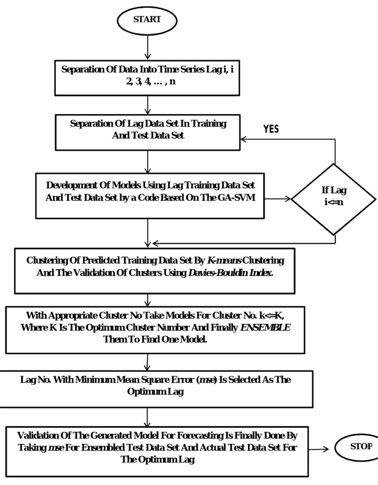
Following steps were followed in the project:

Step 1: The data for reliability of a certain process or machinery was tabulated serially for a

certain period of time.

Step 2: Separation of the data was to be done in to Lag Data. For example if the lag is 2, then the

time series has 2 variables on which the prediction is based.

Step 3: Separation of each of lag data set into training data set and Test data set was done

Step 4: Genetic algorithm and SVM (GA-SVM) was used to run for the lag data set and models

were developed for future prediction.

Step 5: All the models so developed were clustered using k-means clustering to get closely

associated models together.

Step 6: Validation of the clusters was done using Davies-Bouldin Index.

Step 7: For each lag one model from each cluster was selected and then the averaging of these

models into one model is done which is otherwise known as ensemble model.

Step 8: Comparison of the ensembled model was done by taking mean square error (mse) to test

the accuracy with actual data.

(25)

17 YES

Figure 2: Flow chart demonstrating the procedure.

Separation Of Data Into Time Series Lag i, i

ϵ 2, 3, 4, … , n

Separation Of Lag Data Set In Training And Test Data Set

Development Of Models Using Lag Training Data Set

And Test Data Set by a Code Based On The GA-SVM If Lag i<=n Clustering Of Predicted Training Data Set By K-means Clustering

And The Validation Of Clusters Using Davies-Bouldin Index. With Appropriate Cluster No Take Models For Cluster No. k<=K, Where K Is The Optimum Cluster Number And Finally ENSEMBLE

Them To Find One Model.

Lag No. With Minimum Mean Square Error (mse) Is Selected As The Optimum Lag

Validation Of The Generated Model For Forecasting Is Finally Done By Taking mse For Ensembled Test Data Set And Actual Test Data Set For

The Optimum Lag

STOP START

(26)

18

CHAPTER 4 VALIDATION OF MODEL

(27)

19

4. Validation of Developed Model:

To validate the proposed genetic algorithm-based SVM training model, two data sets were used:

1. turbo-charged diesel engine failure data (Pai, 2006; Xu et al., 2003) and

2. computerized numerical control(CNC) machine tool(Feng Ding et al.,2008)

All runs were performed on a 2.2 GHz Intel(R) Dual Core (TM) PC with 2 GB of RAM. All SVM and GA techniques were performed at R-platform.

4.1Reliability forecast of turbochargers in diesel engines

The turbocharger is a vital component in the diesel engine. Reliability information on turbochargers is summarized in the Appendix – I.

In the model developed for GA-SVM, vector of lagged reliability values were taken as input for the model; the corresponding reliability values were considered as the output of the model. The time-series reliability data shown in Eq. (2) are extracted from the reliability data after selecting the lag value p.

Thirty-seven time series data were generated from the reliability data of the Appendix - I after

selecting the p value 3. Out of 37 data, 31 were used as training data for SVM model

development and 6 were selected for testing the model.

Similarly runs were carried out for all lag values ranging from 2 to 10 and the models so developed were saved separately as “training” and “test”.

The models so developed were henceforth clustered using k-means clustering and validated

using Davies-Bouldin index and the minimum value for k was obtained from the graph as shown

(28)

20

Figure 2: graph of Davies-Bouldin index and cluster number for turbo chargers.

With selected cluster number and one model selected from each cluster selected were ensembled to generate a single model. The efficiency or accuracy of the generated model was tested by tabulating the predicted result for training data and actual data and finding their error, absolute error, root mean square error and coefficient of determination as stated in the table below.

Table 1: Error calculation for Turbo chargers diesel engine and CNC machine tool

PARAMETER TURBO CHARGERS DATA

CNC DATA SET MEAN ERROR -5.03E-06 -2.00E-04

ABSOLUTE ERROR 5.55E-05 6.64E-04

MEAN SQUARE ERROR (MSE)

3.86E-09 1.70E-06

ERROR VARIANCE 3.97E-09 1.77E-06

R

2

(29)

21

The training data generated very accurate results but it was previously known to the model. So in order to check the accuracy in predicting future values test data for the optimum lag was introduced and the obtained error calculations for the dumper are given in figure – 4

Figure 3: Actual value versus predicted value for turbo chargers training data

High value of R2 here implies greater accuracy for prediction of the trained data of turbo chargers. Here actual value is the value of output for the optimum lag from collected data.

To see whether the prediction are also better, the actual value and predicted values were also plotted for test data which was not known to the algorithm and same results were obtained as in training data. It is shown in figure-5.

R² = 1 0 0.1 0.2 0.3 0.4 0.5 0.6 0.7 0.8 0.9 1 0.00 0.20 0.40 0.60 0.80 1.00 A C TU A L O U TP U T PEDICTED OUTPUT

(30)

22

Figure 4:Actual value versus predicted value for turbo chargers reliability test data

4.2 Reliability forecasting for CNC machine tool:

Computerized numerical control (CNC) machine tool is the principal equipment in digital manufacturing system of the modern industry. Reliability information on turbochargers is summarized in the Appendix – II.

As in case of turbochargers, in the model developed for GA-SVM, vector of lagged reliability values were taken as input for the model; the corresponding reliability values were considered as the output of the model. The time-series reliability data shown in Eq. (2) are extracted from the reliability data after selecting the lag value p.

Thirty-eight time series data were generated from the reliability data of the Appendix - II

after selecting the p value 3. Out of 38 data, 32 were used as training data for SVM model

development and 6 were selected for testing the model.

The models so developed were henceforth clustered using k-means clustering and

validated using Davies-Bouldin index and the minimum value for k was obtained from

the graph similar to that in for turbo chargers in figure-3.

R² = 1 0.6 0.61 0.62 0.63 0.64 0.65 0.66 0.6 0.61 0.62 0.63 0.64 0.65 0.66 ACT U AL V AL UE PREDICTED VALUE

(31)

23

With selected cluster number and one model selected from each cluster selected were ensembled to generate a single model. The efficiency or accuracy of the generated model was tested by tabulating the predicted result for training data and actual data and finding their error, absolute error, root mean square error and coefficient of determination as stated in the table - I.

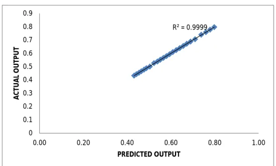
The training data generated very accurate results but it was previously known to the model. So in order to check the accuracy in predicting future values test data for the optimum lag was introduced and the obtained predicted values were plotted against actual values to see the coefficient of determination for the dumper is given in figure – 6.

Figure 5: Actual value versus predicted value for CNC machine tool reliability training data set.

To see whether the validation stands tall with test data set also which was not known to the algorithm, results were as expected and very high accuracy was obtained. It is shown in the figure-7. R² = 0.9999 0 0.1 0.2 0.3 0.4 0.5 0.6 0.7 0.8 0.9 0.00 0.20 0.40 0.60 0.80 1.00 A C TU A L O U TP U T PREDICTED OUTPUT

(32)

24

Figure 6: Actual value versus Predicted value for CNC test data set

R² = 0.9996 0.37 0.38 0.39 0.4 0.41 0.42 0.43 0.37 0.38 0.39 0.40 0.41 0.42 0.43 A C T U A L V A L U E PREDICTED VALUE

(33)

25

CHAPTER 5 CASE STUDY

(34)

26

4. Case Study

The case study for the proposed method involved failure prediction of a dumper in the mining

industry, an industry in which dumper play an important role. Dumper is used for the purpose of carrying the extracted material to its destination for further processing. If a dumper stops then the operation in one part of mine might get affected if spare dumper is not available for allocation or replacement. Therefore, mine management gives full attention to avoiding dumper failure. Historical time-to-failure data for a dumper was collected which constituted of 49 failure data altogether. Cumulative time-to-failure for the dumper was calculated and tabulated in table II.

Table 2: Cumulative time between failure for dumper as case study.

Failure order no Cumulative time

between failure Failure order no

Cumulative time between failure 1 29 26 951.5 2 31.5 27 954.25 3 49 28 980 4 128 29 1002 5 192.5 30 1014.5 6 258 31 1043 7 335.5 32 1187 8 472 33 1327 9 494.25 34 1373 10 501.25 35 1448.75 11 502.25 36 1493.25 12 506.75 37 1495.5 13 519.75 38 1535.5 14 544.75 39 1555.75 15 590.25 40 1580.25 16 613 41 1603 17 659.75 42 1626 18 702.75 43 1645.25 19 707.75 44 1768.25 20 724.5 45 1783.75 21 732 46 1804.25 22 779 47 1820.75 23 901.25 48 1942.25 24 923 49 1967.75 25 925.75

(35)

27

Forty-nine time series data were generated from the reliability data of the table - II after selecting the p

value 3. Out of 49 data, 43 were used as training data for SVM model development and 6 were selected for testing the model.

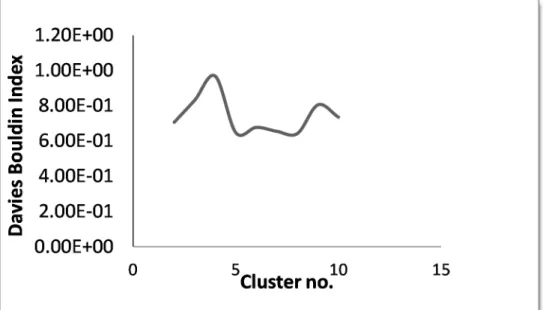
The models so developed were henceforth clustered using k-means clustering and validated using Davies-Bouldin index and the minimum value for k was obtained from the graph as shown below.

Figure 7: Graph of Davies-Bouldin index and cluster number for dumper under case study.

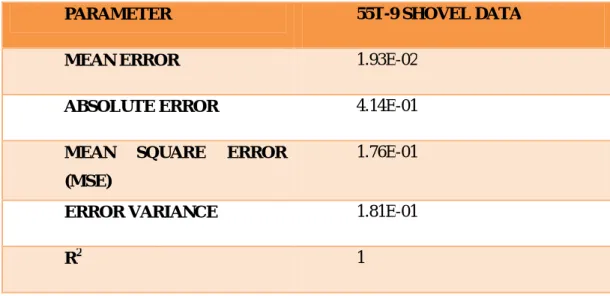
With selected cluster number and one model selected from each cluster selected were ensemble to generate a single model. The efficiency or accuracy of the generated model was tested by tabulating the predicted result for training data and actual data and finding their error, absolute error, root mean square error and coefficient of determination as stated in the table - III.

(36)

28

Table 3: Error calculation table for the dumper under case study.

PARAMETER 55T-9 SHOVEL DATA

MEAN ERROR 1.93E-02

ABSOLUTE ERROR 4.14E-01

MEAN SQUARE ERROR (MSE)

1.76E-01

ERROR VARIANCE 1.81E-01

R2 1

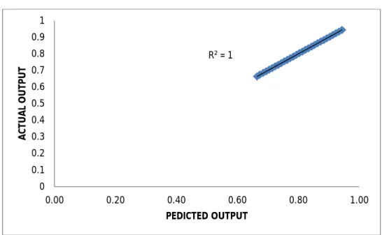
The results for accuracy of developed model for the dumper under case study can be very well incurred from the fig 9

Figure 8: actual value – predicted value for dumper training data.

The training data generated very accurate results but it was previously known to the model. So in order to check the accuracy in predicting future values test data for the optimum lag was introduced and the obtained error calculations for the dumper are given in figure – 10. It is observed form the figure that the predicted value is properly matching with the actual value of the testing data set.

R² = 1 0.00 200.00 400.00 600.00 800.00 1000.00 1200.00 1400.00 1600.00 1800.00 0 500 1000 1500 2000 A C T U A L V A L U E PREDICTED VALUE

(37)

29

Figure 9: actual value – predicted value for dumper test data

R² = 0.9997 6.00E-01 6.10E-01 6.20E-01 6.30E-01 6.40E-01 6.50E-01 6.60E-01 0.6 0.61 0.62 0.63 0.64 0.65 0.66 A C TU A L V A LU E PREDICTED VALUE

(38)

30

CHAPTER 6 CONCLUSIONS

(39)

31

5. CONCLUSIONS:

A genetic algorithm-based SVM model was used for forecasting systems reliability. The number of input variables for this SVM model of reliability plays an important role. The main application of the genetic algorithm was for selection of the SVM parameters. This study shows that selected parameters not only improve the performance of the model but also signiﬁcantly reduce the computational time by eliminating the trial-and-error exercise. I validated the proposed model using two benchmark data sets, and evaluated a comparative study of the predictive performance of various time series models.

The importance of the proposed method is that no a priori speciﬁcations of parametric failure distributions

need to be assumed. Results from the benchmark data sets show that the proposed method performs better than existing methods.

A case study of time-to-failure of a Dumper was conducted. The results of this research clearly demonstrate the potential of this approach for predicting failures and reliability of any system.

(40)

32

CHAPTER 7 REFERENCES

(41)

33 REFERENCES:

Chatterjee, S. and Bandopadhyay, S. (2012). Reliability estimation using a genetic

algorithm-based artiﬁcial neural network: An application to a load-haul-dump machine, Expert Systems

with Applications, http://dx.doi.org/10.1016/j.eswa.2012.03.030.

Ho, S. L., and Xie, M. (1998). The use of ARIMA models for reliability forecasting and analysis.

Computers and Industrial Engineering, 35(1–2), 213–216.

Lu, S., Lu, H., and Kloarik, W. J. (2001). Multivariate performance reliability prediction in

real-time. Reliability Engineering and System Safety, 72, 39–45.

MacKay, D. J. C. (2003). Information theory, inference, and learning algorithms. Cambridge:

Cambridge University Press.

Ding, F., He, Z., Zi, Y., Tan, J., Cao, H., Chen, H. (2008). Application of Support Vector

Machine for Equipment Reliability Forecasting, The IEEE International Conference on Industrial

Informatics, DCC, Daejeon, Korea (526–530).

Zhiwei, G. and Guangchen, B. (2008). Application of Least Squares Support Vector Machine for

Regression to Reliability Analysis, Chinese Journal of Aeronautics 22, 160-166.

Shabri, A.,(2001). Comparison of Time Series Forecasting Methods Using Neural Networks and

Box-jenkins Model, Mathematica, 17(1), 25-32.

Lai, K., Yu, L., Wang, S., Zhou, L. (2006). Credit Risk Analysis Using a Reliability-Based

Neural Network Ensemble Model, ICANN 2006, Part II, LNCS 4132, 682 – 690

Chatterjee, S., Bandopadhyay, S., Machuca, D.(2010). Ore Grade Prediction Using a Genetic

Algorithm and Clustering Based Ensemble Neural Network Model, Math Geosciences, 42: 309–

326.

Golafshani, N.(2003). Understanding Reliability and Validity in Qualitative Research, The

Qualitative Report, 8, 597-607.

Brockwell, P.J. and Richard, A.R., Introduction to Time Series and Forecasting,(2002),Second

(42)

34

Hong, W. C. and Pai, P. F. (2006) Predicting engine reliability by support vector machines, Int J

Adv Manuf Technol, 28, 154–161.

Rocco, S., Moreno, J. (2003). System Reliability Evaluation Using Monte Carlo and Support

Vector Machine, Proceedings of annual reliability and maintainability symposium, 482-486.

(43)

35 APPENDIX:

APPENDIX-I: Reliability(R) data for Turbo Chargers in diesel engines S/L R S/L R 1 0.993 21 0.7938 2 0.9831 22 0.7839 3 0.9731 23 0.7739 4 0.9631 24 0.7639 5 0.9532 25 0.754 6 0.9432 26 0.744 7 0.9333 27 0.7341 8 0.9233 28 0.7241 9 0.9133 29 0.7141 10 0.9034 30 0.7042 11 0.8934 31 0.6942 12 0.8835 32 0.6843 13 0.8735 33 0.6743 14 0.8635 34 0.6643 15 0.8536 35 0.6544 16 0.8436 36 0.6444 17 0.8337 37 0.6345 18 0.8237 38 0.6245 19 0.8137 39 0.6145 20 0.8038 40 0.6046

(44)

36

APPENDIX-II: Reliability(R) data for CNC Machine Tool. i R(ti) i R(ti) i R(ti)

1 0.995 15 0.706 29 0.501 2 0.971 16 0.689 30 0.488 3 0.947 17 0.672 31 0.477 4 0.925 18 0.656 32 0.465 5 0.902 19 0.640 33 0.454 6 0.880 20 0.624 34 0.443 7 0.859 21 0.609 35 0.432 8 0.838 22 0.594 36 0.421 9 0.818 23 0.580 37 0.411 10 0.798 24 0.566 38 0.401 11 0.779 25 0.552 39 0.392 12 0.760 26 0.539 40 0.382 13 0.741 27 0.526 41 0.373

(45)

(46)

(47)