Causal network inference using biochemical kinetics

Causal network inference using biochemical kinetics

Chris J. Oates

*, Frank Dondelinger

, Nora Bayani

, James Korkola

, Joe W. Gray

and

Sach Mukherjee

*

1

Department of Statistics, University of Warwick, Coventry, CV4 7AL,2MRC Biostatistics Unit, Cambridge, CB2 0SR,

UK,3Life Sciences Division, Lawrence Berkeley National Laboratory, Berkeley, CA 94710,4Department of Biomedical

Engineering, Knight Cancer Institute, Oregon Health and Science University, Portland, OR 97239-3098, USA and 5

School of Clinical Medicine, University of Cambridge, Cambridge, CB2 0SP, UK

ABSTRACT

Motivation:Networks are widely used as structural summaries of bio-chemical systems. Statistical estimation of networks is usually based on linear or discrete models. However, the dynamics of biochemical systems are generally non-linear, suggesting that suitable non-linear formulations may offer gains with respect to causal network inference and aid in associated prediction problems.

Results:We present a general framework for network inference and dynamical prediction using time course data that is rooted in non-linear biochemical kinetics. This is achieved by considering a dynam-ical system based on a chemdynam-ical reaction graph with associated kinetic parameters. Both the graph and kinetic parameters are treated as unknown; inference is carried out within a Bayesian framework. This allows prediction of dynamical behavior even when the underlying reaction graph itself is unknown or uncertain. Results, based on (i) data simulated from a mechanistic model of mitogen-activated protein kinase signaling and (ii) phosphoproteomic data from cancer cell lines, demonstrate that non-linear formulations can yield gains in causal network inference and permit dynamical prediction and uncer-tainty quantification in the challenging setting where the reaction graph is unknown.

Availability and implementation:MATLAB R2014a software is avail-able to download from warwick.ac.uk/chrisoates.

Contact:[email protected] or [email protected] Supplementary information:Supplementary data are available at Bioinformaticsonline.

1 INTRODUCTION

Statistical network inference techniques are widely used in the analysis of multivariate biochemical data (Ellis and Wong, 2008; Sachset al., 2005). These techniques aim to make inferences re-garding a networkNwhose vertices are identified with biomole-cular components (e.g. genes or proteins) and edges with (direct or indirect) regulatory interplay between those components.

Network inference methods are typically rooted in linear or discrete models whose statistical and computational advantages facilitate exploration of large spaces of networks (e.g. Ellis and Wong, 2008; Maathuiset al., 2009; Werhliet al., 2006). On the other hand, when the network topology is known, non-linear ordinary differential equations (ODEs) are widely used to model biochemical dynamics (Chen et al., 2009; Kholodenko, 2006). The intermediate case where ODE models are used to select between candidate networks has received less attention.

We propose a general framework called ‘Chemical Model Averaging’ (CheMA) that uses biochemical ODE models to carry out both network inference and dynamical prediction. In summary, we consider a dynamical system dX=dt=f_GðX; Þ

where the state vectorXcontains the abundances of molecular species,Gis a chemical reaction graph that characterizes reac-tions in the system,f_Gis a kinetic model that depends onG, and

collects together all unknown kinetic parameters. A causal net-workNis obtained as a coarse summaryN(G) of the reaction graphGin which each chemical species appears as a single node, and directed edges indicate that the parent is involved in chem-ical reaction(s), which have the child as product (we make these notions precise below). Given time course dataD consisting of noisy measurements ofX, we carry out inference and prediction within a Bayesian framework. In particular, we treatGitself as unknown and make inference concerning it using the posterior distribution, pðGjDÞ /pðGÞ Z pðDj;GÞpðjGÞd |fflfflfflfflfflfflfflfflfflfflfflfflfflfflfflfflffl{zfflfflfflfflfflfflfflfflfflfflfflfflfflfflfflfflffl} marginal likelihoodpðDjGÞ ð1Þ

where the marginal likelihood pðDjGÞ captures how well the chemical reaction graphGdescribes dataD, taking into account both parameter uncertainty and model complexity andpðjGÞis a prior density over the kinetic parameters. In contrast to linear or discrete models that are motivated by tractability, our likeli-hoodpðDj;GÞdepends on (richer) reaction graphsGand their associated kinetics.

This article makes three contributions: (i) A general frame-work for joint netframe-work learning and dynamical prediction using ODE models, (ii) a specific implementation (‘CheMA 1.0’), rooted in Michaelis–Menten kinetics, that uses Metropolis-within-Gibbs sampling to allow Bayesian inference at feasible computational cost and (iii) an empirical investigation, using both simulated and experimental time course data, of the performance of CheMA 1.0 relative to several existing approaches for network inference and dynamical prediction.

The statistical connection betweenlinearODEs and network inference using linear models has been discussed in Oates and Mukherjee (2012) and exploited in Bansalet al.(2006), Gardner et al.(2003). Several approaches based onnon-linearODEs have been proposed, includingAij€€ o and Lahdesm€ aki (2010); Honkela€ et al.(2010); Nachmanet al.(2004); Nelanderet al.(2008). This article extends these ideas by formulating a Bayesian approach to both network inference and dynamical prediction that is rooted in chemical kinetics. Bayesian model selection based on non-linear ODEs has been shown to be a promising strategy for *To whom correspondence should be addressed.

elucidation of specific signaling mechanisms (e.g. Xuet al., 2010). Our work differs in motivation and approach in that we exploit automatically generated rather than hand-crafted biochemical models, thereby allowing full network inference without manual specification of candidate models. Oates et al. (2012) performed Bayesian model selection by comparing steady-state data with equilibrium solutions of automatically generated ODE models. This article extends this approach to time course data and prediction of dynamics.

There are several considerations that motivate CheMA: (i) inference in biological systems is complicated by correlations be-tween components that are co-regulated but not causally linked. It is well known that, under a linear formulation, the causal network N is in general unidentifiable (Pearl, 2009). For ex-ample, it may not be possible to orient certain edges, or edges may be inferred between co-regulated nodes due to strong asso-ciations between them. Non-linear kinetic equations, in contrast, are able to confer asymmetries between nodes and may be suffi-cient to enable orientation of edges (Peterset al., 2011), although we note that causal inference using non-linear models still requires a number of strong assumptions (Pearl, 2009). As a consequence, CheMA can in principle aid in causal network in-ference, and empirical results below support this. (ii) In contrast to linear models, in CheMA, the mechanistic roles of individual variables are respected. This facilitates analysis of data obtained under specific molecular interventions and enhances scientific interpretability. (iii) Prediction of dynamical behavior (e.g. re-sponse to a stimulus or to a drug treatment) in general depends on the chemical reaction graph. In settings where the graph itself is unknown or uncertain (e.g. due to genetic or epigenetic con-text), CheMA allows prediction of dynamics by averaging over an ensemble of (automatically generated) candidate reaction graphs.

The CheMA framework is general and can in principle be used in many settings where kinetic formulations are available to de-scribe the dynamics, including gene regulation, metabolism and protein signaling. For definiteness, in this article, we focus on protein signaling networks mediated by phosphorylation and provide a specific implementation of the general framework. Phosphorylation kinetics have been widely studied (Kholodenko, 2006), and ODE formulations are available, including those based on Michaelis–Menten kinetics (Leskovac, 2003).

The remainder of the article is organized as follows. First, we introduce the model and associated statistical formulation. Second, we discuss network inference and dynamical prediction within this framework. Third, we show empirical results, on simulated and experimental data, comparing CheMA 1.0 with several existing approaches. Finally, we discuss our findings and suggest several directions for further work.

2 METHODS

Below we describe a first implementation of the CheMA framework, called CheMA 1.0, for the specific context of protein phosphorylation networks. Figure 1 provides an outline of the workflow below.

2.1 Automatic generation of reaction graphsG

We construct reaction graphs forpproteinsfX1. . .Xpg=V. EachXican be phosphorylated to X

i; the set of phosphorylated proteins isV

_.

Phosphorylation reactions Xi!Xi are catalyzed by enzymes E2 Ei; the subscript indicates that each protein may have a specific set of en-zymes (kinases). We consider the case in which the kinases themselves are phosphorylated proteins, i.e.Ei V (if phosphorylation ofXi is not driven by an enzyme inV_{, we setE}

i=1). For simplicity, we do not consider multiple phosphorylation sites, other post-translational modifi-cations (e.g. ubiquitinylation), protein degradation or spatial effects. The ability of enzymeE2 Ei to catalyze phosphorylation ofXimay be in-hibited by proteinsI2 Ii;E V; the double subscript indicates that in-hibition is specific to both targetXiand enzymeE(see below).

The reaction graph G provides a visual representation of the sets Ei andIi;E; Figure 1 shows an illustrative example on three proteins A, B and C. A causal biological network N(G) is formed by drawing exactlypvertices and edges (i,j) indicating thatX

i is either an enzyme catalyzing phosphorylation ofXj, or an inhibitor of such an enzyme. That is, ði;jÞ 2N,i2 Ej_ 9Ei2 Ij;E. For the example shown in Figure 1, the corresponding network N is the directed graph

A!C B.

2.2 Automatic generation of kinetic modelsfG

The reaction graphGcan be decomposed into local graphsGidescribing enzymes (and their inhibitors) for phosphorylation of proteinXi. For simplicity of exposition, we consider inference concerningGi. Thus,Xi

plays the role of the substrate; following conventional notation in enzyme kinetics, we refer toXiusing the symbolSand use [] to denote concen-tration of the chemical species indicated by the argument.

We use kinetic models fG based on Michaelis–Menten functionals (Leskovac, 2003). Here we restrict attention to a relatively simple model class, but more complex dynamics could be incorporated. The rate of phosphorylation due to kinase E is given by VE½E½Sh=ð½Sh+KhEÞ, which acknowledges variation of kinase concentration [E] and permits kinase-specific response profiles, parameterized byKEandh, with rate constantVE. Below, the Hill coefficienthis taken equal to 1 (non-coopera-tive binding). We consider competi(non-coopera-tive inhibition, where substrate and inhibitor I compete for the same binding site on the enzyme (EIÐEÐES!E+S_{). When multiple inhibitors are present, they} are assumed to act exclusively, competing for the same binding site on

Fig. 1.CheMA. Chemical reaction graphsGsummarize interplay that is described quantitatively by kinetic equationsf_G. Candidate graphsGare scored against observed time course dataDin a Bayesian framework. A networkN gives a coarse summary of the system; marginal posterior probabilities of edges inNquantify evidence in favor of causal relation-ships. The reaction graphG(andN) is treated as an unknown, latent object and the methodology allows Bayesian prediction of dynamics (including under intervention) in the unknown graph setting

the enzyme (EIÐEÐEI0_{), corresponding mathematically to a rescaling} of the Michaelis–Menten parameterKE°KEð1+PI2IS;E½I=KIÞ. We do not model phosphatase specificity; in particular, dephosphorylation is assumed to occur at a rate V0½S=ð½S+K0Þ, depending on a Michaelis–Menten parameterK0and taking a maximal valueV0.

Combining these assumptions produces a kinetic model for phosphor-ylation of substrateS, given byfG;SðX; SÞ=

V0½S ½S_+K 0 +X E2ES VE½E½S ½S+KE 1+ X I2IS;E ½I KI ! ð2Þ

where the parameter vector S contains the maximum rates V and Michaelis–Menten constantsK, and the (local) graphGSspecifies the setsESandIS;E. The complete dynamical systemfGis given by taking, for each speciesS2 V, a model akin to Equation (2). In this way, we are able to automate the generation of candidate parametric ODE models.

2.3 Model averaging and the networkN

Evidence for a causal influence of proteinion proteinjis summarized by the marginal posterior probability of a directed edge (i,j) in the network

N. This is obtained by averaging over all possible reaction graphsG, as

pðði;jÞ 2NjDÞ= X G:i2Gj pðDjGÞpðGÞ X G pðDjGÞpðGÞ: ð3Þ We note that while the marginal posterior in Equation (3) is an intuitive summary, the full posterior over reaction graphsG is also available for more detailed exploration. In the same vein, model averaging is used to compute posterior predictive distributions (see Supplementary Material).

Following work in structural inference for graphical models (Ellis and Wong, 2008), we bound graph in-degree; in particular, we consider only those sets of kinasesES V that satisfyjESj c1, and similarly, we bound the number of inhibitorsjIS;Ej c2(see Section 3.1 below).

Bayesian variable selection requires multiplicity correction to control the false discovery rate and avoid degeneracy (Scott and Berger, 2010). For phosphorylation networks, we achieve multiplicity correction using a priorp(G) uniform over the number of kinases, and for a given kinase, uniform over the number of kinase inhibitors:

pðGÞ=Y p i=1 p jEij !1 Y E2Ei p jIi;Ej !1 ð4Þ

We note that the above prior does not include biological knowledge concerning specific edges; informative structural priors are also available in the literature (Mukherjee and Speed, 2008).

2.4 Statistical formulation: CheMA 1.0

2.4.1 Time course data DataDcomprise measurementsyiðtjÞandyi ðtjÞproportional to the concentrations of unphosphorylated and phos-phorylated forms, respectively, of proteiniat discrete timestj, 0jn. Data are scale normalized to give unit mean for each protein (P_jyiðtjÞ=PjyiðtjÞ=n+1). In CheMA 1.0, observables are related to dynamics via ‘gradient matching’. We follow Aij€ o and L€ ahdesm€ aki€ (2010); Bansalet al. (2006); Oates and Mukherjee (2012) and use a simple Euler scheme that approximates the gradientdXi=dtat time tj byziðtjÞ=ðyiðtjÞ yiðtj1ÞÞ=ðtjtj1Þ. We note that more accurate ap-proximations could be used, at the cost of requiring more data points or additional modeling assumptions (see Section 4). The ODE modelfG;S [Equation (2)] is formulated as a statistical model by constructing, con-ditional upon (unknown) Michaelis–Menten parameters K, a design

matrixDG;SðKÞwith rows

" y S y S+K0 ;. . .; y EyS yS+KE 1+P I2IS;E y I KI |fflfflfflfflfflfflfflfflfflfflfflfflfflfflfflfflfflfflfflfflfflfflfflffl{zfflfflfflfflfflfflfflfflfflfflfflfflfflfflfflfflfflfflfflfflfflfflfflffl} ;. . . E2ES # ð5Þ

and then interpreting Equation (2) statistically as

zS=DG;SðKÞV+; N ð0; 2IÞ ð6Þ wherezS=½zSðt1Þ;. . .;zSðtnÞT;Ndenotes a normal density,2the noise variance,Ithe identity matrix and, as above,Vis the vector of maximum reaction rates. The appropriateness of normality, additivity and the uncorrelatedness of errors necessarily depends on the data generating and measurement processes, as well as the time intervalstjtj1between consecutive observations, as discussed in Oates and Mukherjee (2012). This approximation has the crucial advantage of rendering the local re-action graphsGS statistically orthogonal, such that each may be esti-mated independently (see Hillet al., 2012). Iterating overS2 Vpermits inference concerning the complete reaction graphG.

2.4.2 MCMC and marginal likelihoods CheMA 1.0 uses truncated normal priorsNTð;SÞwith parameters;Sinherited from the corres-ponding untruncated distribution. Truncation ensures non-negativity of parameters, while normality facilitates partial conjugacy (see below); add-itional information on truncated normals is provided in the Supplementary Material. To simplify notation, we consider a specific variableSand candidate modelGSand omit the subscript in what fol-lows. To elicit hyperparameters;S, we follow Xuet al. (2010) and assume all processes occur on observable time and concentration scales, that is_V; _K Oð1Þ, reflecting that the data are normalized a priori. For prior covariance of Michaelis–Menten parametersSK, we assume independence of the components Ki, so that pðKÞ=NTðK;K; IÞ, whereK; are hyperparameters. For the prior covarianceSVof max-imum reaction rates, we take a unit information formulation of the trun-cated g-prior, so that pðVjK; Þ=NTðV;V;n2ðD0DÞ1Þ where D=DG;SðKÞis the design matrix defined above. This implies that the prior contributes (approximately) the same amount of information as one data point, as recommended by Kass and Wasserman (1995), and automatically selects the scale of the prior covariance (see Zellner, 1986). For the noise parameter, we use a Jeffreys priorpðÞ /1=. These latter choices render the formulation partially conjugate, permitting an efficient Metropolis-within-Gibbs Markov chain Monte Carlo (MCMC) sampling scheme for the parameter posterior distribution, as described in detail in the Supplementary Material.

To estimate marginal likelihoods from sampler output, we exploit par-tial conjugacy and use the method of Chib and Jeliazkov (2001). As inference in CheMA 1.0 decomposes over proteinsXi2 V, and for a given protein, over local modelsGi, the computations were parallelized (full details and software provided as Supplementary Material). Alternatively, MCMC could be used over the discrete space of reaction graphs (Ellis and Wong, 2008) or the joint space of graphs and param-eters (Oateset al., 2012).

2.4.3 Interventions on the system In interventional experiments, data are obtained under treatments that externally influence network edges or nodes. Inhibitors of protein phosphorylation are now increas-ingly available; such inhibitors typically bind to the kinase domain of their target, preventing enzymatic activity. We consider such inhibitors in biological experiments below. Within CheMA 1.0, we model inhibition by setting to zero those terms in the design matrixDG;Scorresponding to the inhibited enzymeEin the treated samples (‘perfect certain’ interven-tions in the terminology of Eaton and Murphy, 2007; Spenceret al., 2012). This removes the causal influence ofEfor the inhibited samples.

3 RESULTS

3.1 Hyperparameter specification and sensitivity

For CheMA 1.0, we set hyperparameters _V=_K=1; =1=2 and the maximum in-degree constraintc1=2; we investigated sensitivity by varying these parameters within (i) a toy model of signaling (Supplementary Fig. S3a–c) and (ii) in a subset of the simulations reported below (Supplementary Fig. S2). As the action of inhibition is second order in the Taylor expansion sense, inference for inhibitor variablesIS;E may be expected to require substantially more data, in line with the ‘weak identifiability’ of second-order terms reported in Calderhead and Girolami (2011). A preliminary investigation based on a toy model of signaling revealed that at typical sample sizes in-ference for inhibitor sets I_S;E was extremely challenging (Supplementary Fig. S3d). Combined with computational con-siderations, we decided to fixc2=0 for subsequent experiments; that is, we did not include inhibitory regulation in the reaction graph. Further diagnostics, including MCMC convergence, are presented in the Supplementary Material.

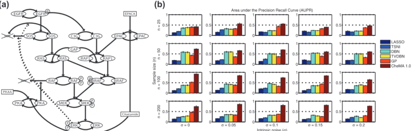
3.2 In silicoMAPK pathway

Data were generated from a mechanistic model of the MAPK signaling pathway described by Xuet al.(2010), specified by a system of 25 ODEs of Michaelis–Menten type whose reaction graph is shown in Figure 2a. This archetypal protein signaling system provides an ideal test bed, as the causal graph is known, and the model has been validated against experimentally ob-tained data (Xuet al., 2010). Following Oates and Mukherjee (2012), the Xuet al.model was transformed into a stochastic differential equation with intrinsic noise . Full details of the simulation setup appear in Supplementary Material.

For inference of the network N(G), we compared our ap-proach with existing network inference methods that are com-patible with time course data: (i) ‘1-penalized regression (‘LASSO’), (ii) time series network identification (‘TSNI’;

Bansal et al.2006; this is based on‘2-penalized regression), (iii) dynamic Bayesian networks (‘DBN’; Hillet al., 2012), (iv) time-varying DBNs (Dondelingeret al., 2012) and (v) Gaussian pro-cess regression with model averaging (‘GP’; Aij€€ o and L€ahdesm€aki, 2010). Approaches (i–iii) are based on linear differ-ence equations; (iv) relaxes the linear assumption in a piecewise fashion, whereas (v) is a semiparametric variable selection tech-nique. We note that because TSNI cannot deal with multiple time courses, we adapted it for use in this setting. Implementa-tion details for all methods may be found in the Supplementary Material.

To systematically assess estimation of network structure, we computed the average area under the precision-recall (AUPR) and area under the receiver-operating characteristic (AUROC) curves. Figure 2b shows mean AUPR for all approaches, for 20 regimes of sample sizenand noise. CheMA 1.0 performs con-sistently well in all regimes, and outperforms (i–v) substantially at the larger sample sizes. It is interesting to note that the linear and piecewise linear DBNs (iii–iv) perform better at moderate sample sizes compared with higher sample sizes, possibly because of model misspecification. AUROC results (Supplementary Fig. S6) showed a broadly similar pattern, with CheMA 1.0 offering gains at larger sample sizes. For the kinetic parameters, however, we found that CheMA 1.0 struggled to precisely re-cover the true values=fV;Kg, even when the reaction graph Gwas known (Fig. 3). The posterior distribution over rate con-stantsVwas much more informative than the posterior distribu-tion over Michaelis–Menten parameters K, consistent with the ‘weak identifiability’ of kinase inhibitors that we found in Section 3.1.

To investigate dynamical prediction in the setting where nei-ther reaction graph nor parameters are known, we generated data from an unseen intervention and assessed ability to predict the resulting dynamics (details of the simulation are included in the Supplementary Material). To fix a length scale, both true and predicted trajectories were normalized by maximum protein 0 0.5 1 n = 25 0 0.5 1 0 0.5 1

Area under the Precision Recall Curve (AUPR)

0 0.5 1 0 0.5 1 0 0.5 1 Sample size (n) n = 50 0 0.5 1 0 0.5 1 0 0.5 1 0 0.5 1 LASSO TSNI DBN TVDBN GP CheMA 1.0 0 0.5 1 n = 100 0 0.5 1 0 0.5 1 0 0.5 1 0 0.5 1 0 0.5 1 σ = 0 n = 200 0 0.5 1 σ = 0.05 0 0.5 1 σ = 0.1 Intrinsic noise (σ) 0 0.5 1 σ = 0.15 0 0.5 1 σ = 0.2 (b) (a)

Fig. 2.Network inference, simulation study. (a) Reaction graphGfor the MAPK signaling pathway because of Xuet al.(2010). (The model, based on enzyme kinetics, uses Michaelis–Menten equations to capture a variety of post-translational modifications including phosphorylation.) (b) AUPR[with respect to the true causal networkN(G)] for varying sample sizenand noise level. [Network inference methods: (i) LASSO,‘1-penalized regression, (ii) TSNI,‘2-penalized regression, (iii) DBN, dynamic Bayesian networks, (iv) TVDBN, time-varying DBNs, (v) GP, non-parametric regression, (vi) CheMA 1.0, based on chemical kinetic models. Error bars display standard error computed over five independent datasets. (Full details provided in Supplementary Material.)

expression in the test data. The quality of a predicted trajectory was then measured by the mean squared error (MSE) relative to the (held out) data points. The network inference approaches (i– v) above cannot be directly applied for prediction in this setting (although they could in principle be adapted to do so). Therefore, we compared CheMA 1.0 with the analogous linear formulation, that replaces Equation (2) by fG;SðX; SÞ=0+

P

E2ESE½X

E (see Supplementary Material for details), along

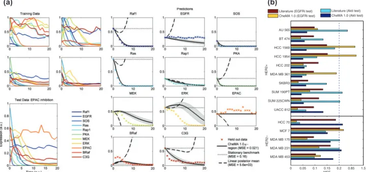
with a simple, baseline estimator (the ‘stationary benchmark’) that presumes protein concentrations do not change with time. Figure 4a displays predictions for the dynamics that result from EPAC inhibition. Here CheMA 1.0 provides qualitatively correct prediction, whereas the linear analogue rapidly diverges to infin-ity (due to poorly estimated eigenvalues). Therefore, we focused only on short-term prediction, specifically the first 25% of the time course, for which linear models may yet prove useful. Over all simulation regimes and experiments, including at small sample sizes, we found that our approach produced significa-ntly lower MSE than both the linear and benchmark mo-dels (MSECheMA 1:0=0:061;MSELin:=2:55;MSEBench:=0:199). Furthermore, CheMA 1.0 consistently produced lowest MSE at all fixed values of n and (Supplementary Fig. S10; P50.001 binomial test).

3.3 In Vitro signaling

Next, we considered experimental data obtained using reverse-phase protein arrays (Hennessy et al., 2010) from 15 human breast cancer cell lines, of which 10 were of HER2+ subtype (Neveet al., 2006). These data comprised observations for key phosphoproteins AKT, EGFR, MEK, GSK3ab, S6, 4EBP1 and their unphosphoryated counterparts. Data were acquired under pretreatment with inhibitors Lapatinib (‘EGFRi’; an EGFR/ HER2 inhibitor), GSK690693 (‘AKTi’; an AKT inhibitor) and without inhibition (DMSO) at 0.5, 1, 2, 4 and 8 h following serum stimulation, giving n= 15 observations of each species in each cell line (see Supplementary Material for full experimen-tal protocol). UACC 812 SUM 225CWN SUM 190PT SKBR3 MDA MB 361 HCC 202 HCC 1954 HCC 1569 BT 474 AU 565 HER2+

Literature (Akti test) CheMA 1.0 (Akti test)

0 0.05 0.1 0.15 0.2 0.85 1.5 MDA MB 453 MDA MB 231 MDA MB 175 MCF 7 HCC 70 MSE HER2−

Literature (EGFRi test) CheMA 1.0 (EGFRi test)

(a) (b)

Fig. 4. Predicting dynamical response to a novel intervention: (a) predicting the effect of EPAC inhibition under the data generating model of Xuet al.

(2010). [CheMA (solid) regions correspond to standard deviation of the posterior predictive distribution. Linear (dashed) replaces the non-linear chemical kinetic models with simple linear models. The stationary benchmark (dotted) simply uses the initial data point as an estimate for all later data points. The true test data are displayed as crosses. Heren= 100,=0:1.] (b) Assessing prediction over a panel of 15 breast cancer cell lines. (Training data were time series under treatment with a single inhibitor; test data represented a second held-out inhibitor. Normalized MSE was averaged over all protein species and all time points.)

0 5 10 0 0.5 1 1.5 V₀ pdf 0 5 10 0 0.2 0.4 0.6 0.8 V₁ 0 5 10 0 0.2 0.4 0.6 0.8 V₂ 0 5 10 0 0.2 0.4 0.6 0.8 K₀ pdf 0 5 10 0 0.2 0.4 0.6 0.8 K₁ 0 5 10 0 0.2 0.4 0.6 0.8 K₂ 0 5 10 0 0.2 0.4 0.6 0.8 K₃ n=3 n=5 n=10 true

Fig. 3.Posterior distributions over kinetic parameters when the graphG

is known. As the number of samplesn increases, the posterior mass concentrates on the true values much faster for the maximum reaction ratesV(top row) than for the Michaelis–Menten parametersK(bottom row)

Assessment of inferred network topologies for the cell lines is challenging because the true cell line-specific networks are not known. Inferred topologies partially agree with known signaling (Supplementary Fig. S11), but the latter is based mainly on stu-dies using wild-type cells and may not reflect networks in genet-ically perturbed cancer lines. Therefore, to assess performance, we also considered the problem of prediction of trajectories under an unseen intervention, where objective assessment is pos-sible. We sought to compare performance of CheMA 1.0 against a literature-based ODE model (reaction graphGfixed according to literature and dynamicsfGas described above) fitted to train-ing data. No prior information concerntrain-ing specific chemical reactions was provided to CheMA 1.0. This problem is highly non-trivial because of the small sample size, uneven sampling times and the complex observation process associated with prote-omic assay data.

Training on DMSO and EGFRi (or AKTi) data, we assessed ability to predict the full dynamic response to AKT (or EGFR) inhibition. In this way, each held-out test set contained trajec-tories under a completely unseen intervention. By considering all 15 cell lines, giving 30 held-out datasets, we found that in 19 of 30 prediction problems CheMA 1.0 outperformed the literature predictor (Fig. 4b). As expected (and as in the case of the simu-lated data), the linear model was not well behaved for prediction (Supplementary Fig. S12) and is not shown. In the AKTi test, of the 10 HER2+ cell lines, 9 were better predicted by CheMA 1.0 compared with literature prediction (P= 0.01, binomial test; MSECheMA 1:0=0:064 versus MSELit:=0:274). Conversely, four of five HER2– lines were better predicted by literature (MSELit:=0:145 versus MSECheMA 1:0=0:240), suggesting that signaling network topology in HER2+ lines may differ to the (wild type) literature topology, in line with the literature on the cell lines (Neveet al., 2006). This is encouraging from the per-spective of CheMA, as a priori it is far from clear whether the training data, which involved onlyP= 6 species andn= 10 data points, contain sufficient information to predict the effect of an unseen intervention, even approximately. However, in two of the failure cases (HCC 1569, HCC 1954; EGFRi test) CheMA 1.0 produced extremely poor predictions (MSECheMA 1:041), likely because of the small training sample size.

4 DISCUSSION

We proposed a general framework for using chemical kinetics in network inference and dynamical prediction. The use of chemical kinetics can be expected to contribute gains in causal inference because the underlying models are not structurally symmetric, allowing causal directionality to be established (Peters et al., 2011). In empirical results, we found that while CheMA 1.0 struggled to identify kinetic parameters from data, it was never-theless able to identify the causal network; this discrepancy is explained by the fact that the latter is in a sense a projection of the former, and can be identifiable even when the full set of parameters are not.

An important challenge in systems biology is to predict the effect on signaling of a novel intervention, such as a drug treat-ment. At present, dynamical predictions in systems biology re-quire a known chemical reaction graph, for instance, taken from the literature; a system of ODEs is usually specified based on

such a graph and used for prediction. However, in many settings, the chemical reaction graph may differ depending on cell type or disease state and cannot be assumed known. In contrast, CheMA shows how prediction of dynamical behavior may be possible even when the reaction graph itself is unknown a priori. Unlike more convenient linear or discrete formulations, our use of chemical kinetic models provides interpretable predictions. For example, the dynamic behavior of phosphoprotein concen-trations obtained under chemical kinetic rate laws is physically plausible (i.e. smooth, bounded and non-negative). Furthermore, by averaging predictions over reaction graphs, our approach should provide robustness in (typical) situations where it is un-reasonable to expect to identifyG precisely. Nevertheless, pre-diction of trajectories based on the protein data was challenging, likely because of noise and small sample sizes (Supplementary Fig. S13). We anticipate that continuing technical advances will move high-throughput proteomics closer to the favorable simu-lation regimes in Section 3.2 on which we found the richer non-linear models to be useful.

Several improvements can be made to the CheMA 1.0 imple-mentation reported here, of which we highlight two: (i) gradient matching (rather than numerical solution of the automatically generated dynamical systems) can help to relieve the computa-tional demands associated with exploration the large model spaces, but the Euler approximations we used for this purpose are crude. Improved gradient matching should be possible (at the expense of requiring more time points) via higher-order expan-sions, or (at the expense of additional modeling assumptions) kernel regression, the penalized likelihood approaches of Gonzalez et al.(2013); Ramsay et al.(2007), or the Bayesian approach of Dondelinger et al. (2013). (ii) CheMA 1.0 does not explicitly distinguish between process noise and observation noise; an interesting direction for further research would be to incorporate an explicit observation model.

Two ongoing challenges in Bayesian computation relevant to CheMA include inference of model parameters and computation of marginal likelihoods for model selection. The second is an active area of research, with candidate approaches including variational approximations (Rue et al., 2009) and MCMC (Vyshemirsky and Girolami, 2008). In general, the computa-tional burden of CheMA will be higher than many methods (see Supplementary Material). By way of illustration, Bayesian inference and prediction for a system of 27 protein species re-quired over 12 h (serial) computational time. In contrast, linear or discrete models offer better scalability to high-dimensional settings. Thus, CheMA can complement existing methodologies but is not at present applicable to truly high-dimensional prob-lems with hundreds or thousands of nodes.

Finally, we note the following caveats: (i) the automatic gen-eration of kinetic equations limits the extent to which detailed knowledge about particular biochemical processes and dynamics may be incorporated. (ii) Our empirical results suggest that more complex interactions, including kinase inhibition, can be ex-tremely difficult to identify in practice. (iii) The form of kinetics used here will likely be suboptimal when the assumptions of the Michaelis–Menten approximation are violated. (iv) Larger train-ing and test datasets may be needed to allow truly effective trajectory prediction and comprehensive assessment of performance.

Funding: US Department of Energy (DE-AC02-05CH11231); US National Institute of Health, National Cancer Institute (U54 CA 112970, P50 CA 58207); UK Engineering and Physical Sciences Research Council (EP/E501311/1); and Netherlands Organisation for Scientific Research [Cancer Systems Biology Center].

Conflicts of interest: none declared.

REFERENCES

€

Aij€o,T. and L€ahdesmaki,H. (2010) Learning gene regulatory networks from gene€ expression measurements using non-parametric molecular kinetics. Bioinformatics,25, 2937–2944.

Bansal,M.et al. (2006) Inference of gene regulatory networks and compound mode of action from time course gene expression profiles.Bioinformatics,22, 815–822. Calderhead,B. and Girolami,M. (2011) Statistical analysis of nonlinear dynamical systems using differential geometric sampling methods.J. R. Soc. Interface Focus,1, 821–835.

Chen,W.W.et al. (2009) Input-output behavior of ErbB signaling pathways as revealed by a mass action model trained against dynamic data.Mol. Syst. Biol.,5, 239.

Chib,S. and Jeliazkov,I. (2001) Marginal likelihood from the metropolis-hastings output.J. Am. Stat. Assoc.,96, 270–281.

Dondelinger,F.et al. (2012) Non-homogeneous dynamic Bayesian networks with Bayesian regularization for inferring gene regulatory networks with gradually time-varying structure.Mach. Learn.,90, 191–230.

Dondelinger,F.et al. (2013) ODE parameter inference using adaptive gradient matching with Gaussian processes. In:Sixteenth International Conference on Artificial Intelligence and Statistics,Scottsdale, AZ, USA. pp. 216–228. Eaton,D. and Murphy,K. (2007) Exact Bayesian structure learning from uncertain

interventions. In:11th International Conference on Artificial Intelligence and Statistics. Vol. 2, pp. 107–114.

Ellis,B. and Wong,W. (2008) Learning causal bayesian network structures from experimental data.J. Am. Stat. Assoc.,103, 778–789.

Gardner,T.et al. (2003) Inferring genetic networks and identifying compound mode of action via expression profiling.Science,301, 102–105.

Gonzalez,J.et al. (2013) Inferring latent gene regulatory network kinetics.Stat. Appl. Genet. Mol.,12, 109–127.

Hennessy,B.T.et al. (2010) A technical assessment of the utility of reverse phase protein arrays for the study of the functional proteome in nonmicrodissected human breast cancer.Clin. Proteomics,6, 129–151.

Hill,S.M.et al. (2012) Bayesian inference of signaling network topology in a cancer cell line.Bioinformatics,28, 2804–2810.

Honkela,A.et al. (2010) Model-based method for transcription factor target iden-tification with limited data.Proc. Natl Acad. Sci. USA,107, 7793–7798.

Kass,R.E. and Wasserman,L. (1995) A reference Bayesian test for nested hypoth-eses and its relationship to the Schwarz criterion. J. Am. Stat. Assoc.,90, 928–934.

Kholodenko,B. (2006) Cell-signalling dynamics in time and space.Nat. Rev. Mol. Cell Biol.,7, 165–176.

Leskovac,V. (2003)Comprehensive Enzyme Kinetics. Kluwer Academic/Plenum Publishers, New York.

Maathuis,M.H.et al. (2009) Estimating high-dimensional intervention effects from observational data.Ann. Stat.,37, 3133–3164.

Mukherjee,S. and Speed,T. (2008) Network inference using informative priors. Proc. Natl Acad. Sci. USA,105, 14313–14318.

Nachman,I.et al. (2004) Inferring quantitative models of regulatory networks from expression data.Bioinformatics,20, i248–i256.

Nelander,S.et al. (2008) Models from experiments: combinatorial drug perturb-ations of cancer cells.Mol. Syst. Biol.,4, 216.

Neve,R.et al. (2006) A collection of breast cancer cell lines for the study of func-tionally distinct cancer subtypes.Cancer Cell,10, 515–527.

Oates,C.J. and Mukherjee,S. (2012) Network inference and biological dynamics. Ann. Appl. Stat.,6, 1209–1235.

Oates,C.J.et al. (2012) Network inference using steady state data and Goldbeter-Koshland kinetics.Bioinformatics,28, 2342–2348.

Pearl,J. (2009) Causal inference in statistics: an overview.Stat. Surv.,3, 96–146. Peters,J.et al. (2011) Identifiability of causal graphs using functional models. In:

27th Conference on Uncertainty in Artificial Intelligence, Barcelona, Spain. pp. 589–598.

Ramsay,J.O. (2007) Parameter estimation for differential equations: a generalized smoothing approach.J. R. Stat. Soc. Series B Stat. Methodol.,69, 741–796.

Rue,H.et al. (2009) Approximate Bayesian inference for latent Gaussian models using integrated nested laplace approximations.J. R. Stat. Soc. Series B Stat. Methodol.,71, 319–392.

Sachs,K.et al. (2005) Causal Protein-signaling networks derived from multipara-meter single-cell data.Science,308, 523–529.

Scott,J.G. and Berger,J.O. (2010) Bayes and empirical-bayes multiplicity adjustment in the variable-selection problem.Ann. Stat.,38, 2587–2619.

Spencer,S.E.F.et al. (2012) Dynamic Bayesian networks for interventional data. In: CRiSM Working Paper. University of Warwick, Coventry, UK.

Vyshemirsky,V. and Girolami,M. (2008) Bayesian ranking of biochemical system models.Bioinformatics,24, 833–839.

Werhli,A.et al. (2006) Comparative evaluation of reverse engineering gene regula-tory networks with relevance networks, graphical Gaussian models and Bayesian networks.Bioinformatics,22, 2523–2531.

Xu,T.-R. et al. (2010) Inferring signaling pathway topologies from multiple perturbation measurements of specific biochemical species. Sci. Signal., 3, ra20.

Zellner,A. (1986) On assessing prior distributions and Bayesian regression analysis with g-prior distributions. In: Goel,P.K. and Zellner,A. (eds)Bayesian inference and decision techniques—Essays in honor of Bruno de Finetti,North-Holland, Amsterdam. pp. 233–243.