University of Colorado, Boulder
CU Scholar
Undergraduate Honors Theses
Honors Program
Spring 2015
Finite Sample Performance of Semiparametric
Estimation Methods for Partially Linear Models
Under Nonparametric Endogeneity
David Anderson
Follow this and additional works at:
http://scholar.colorado.edu/honr_theses
Part of the
Econometrics Commons
This Thesis is brought to you for free and open access by Honors Program at CU Scholar. It has been accepted for inclusion in Undergraduate Honors Theses by an authorized administrator of CU Scholar. For more information, please [email protected].
Recommended Citation
Anderson, David, "Finite Sample Performance of Semiparametric Estimation Methods for Partially Linear Models Under Nonparametric Endogeneity" (2015).Undergraduate Honors Theses.Paper 900.
Finite Sample Performance of Semiparametric Estimation Methods for
Partially Linear Models Under Nonparametric Endogeneity
David Anderson
Department of Economics
University of Colorado
Boulder, CO 80309-0256, USA
email: [email protected]
Voice: + 1 408 348 8725
Abstract. In this paper we discuss the derivation, and use a Monte Carlo study to examine the finite sample performances of select estimators put forth in Martins-Filho et al. (2015) for partially linear semiparametric models under nonparametric endogeneity. We find that the selected estimators sufficiently account for the explicit nonparametric endogeneity of the underlying model in finite samples, and conclude that the proposed estimators ˆm(x) and p are more efficient than their counterparts ˜m(x) and wp. Our findings support the
assertion that the estimators form(x) are oracle efficient.
Keywords and phrases. Semiparametric regression, Nonparametric endogeneity, Monte Carlo
JEL classifications. C14, C15
Defended March 31, 2015
Thesis Advisor
Carlos Martins-Filho|Department of Economics
Defense Committee
Martin Boileau|Department of Economics |Honors Council Representative Jem Corcoran|Department of Applied Mathematics
1
Introduction
Semiparametric estimation methods combine the precision of parametric methods and the flexibility of non-parametric estimation. Although quite desirable for their minimal assumptions, nonnon-parametric estimation methods su↵er from the curse of dimensionality and are not feasible for large dimensional regressors. As a result, it may be desirable to combine parametric and nonparametric assumptions to construct flexible yet easy to estimate models.
The curse of dimensionality in nonparametric regression is most easily illustrated by examining the optimal convergence rates put forth in Stone (1982). He derives the optimal rate of convergence, n r, of
an estimator ˆ✓(X) to the true p-times di↵erentiable regression function ✓(X) as r = p/(2p+D) where
X 2RD. Clearly the rate of convergence of nonparametric estimation has an inverse relationship with the
dimensionality ofX, requiring a much larger sample sizenor strong assumptions about the di↵erentiability
of the underlying functional form for the same precision obtainable from a lower dimensional regressor. One restriction we can impose on a fully nonparametric model to solve the curse of dimensionality is additivity, i.e. some object of estimationf(X) whereX 2 RD can be written as PD
d=1
gd(Xd), where Xd is
the d-th component of X. As illustrated above, if we can impose this restriction, the convergence rates
estimators is much faster in this additive structure than we would have otherwise. The convergence rate of this specific additive structure isr=p/(2p+ 1), and is examined further in Stone (1985).
In the model we examine in this paper, we restrict the object of estimation to be partially linear and ad-ditive, in a combination of parametric and nonparametric assumptions mentioned earlier. These restrictions result in the semiparametric model Y = Zs0 +m(X) +" for some conformable vectors Zs, X and some
scalarsY,". This is the standard semiparametric model first popularized by Robinson (1988), and has been
considered under a variety of relaxed assumptions and additional structure.
For the model examined in this paper, we add the an auxiliary equation as in Newey et al. (1999) to account for the explicit nonparametric endogeneity assumption E("|X)6= 0. We add the assumption that
X =g(Z) +U whereY 2R,X 2RD,Z
2RL and the previously definedZsis a subvector ofZ, Zs
and L1 < L. Estimators for models with this structure have been examined by Martins-Filho and Yao
(2012) who examined the case where both the parametric and nonparametric regressors are endogenous, and Gao and Phillips (2013) who consider the model where the parametric portion is endogenous and the nonparametric portion is strictly non stationary.
In this paper we present the derivation of some selected estimators for andm(X) proposed by
Martins-Filho et al. (2015), and use a Monte Carlo study to examine the finite sample performance under a varying number data generating procedure designs.
2
Literature Review
Our interest begins with Robinson (1988) which outlays a pn - consistent estimator for for the model
Y =Zs0 +m(X) +"whereE("
|X) = 0. For some observed sample{(Yi, Zi1,· · · , ZiL1, Xi1,· · · , XiD)}
n i=1 of some sample sizen, denoteY0 = (Y1· · ·Yn), Z= (Zi,l)in,L=11,l=1 andX= (Xi,d)n,Di=1,d=1 and let Ai. denote
theith row of some matrixA. His method estimated as ˆ =h1 n n X i=1 (Zi. Zˆi.)0(Zi. Zˆi.) i 1h1 n n X i=1 (Zi. Zˆi.)0(Yi Yˆi) i
where ˆZi and ˆYi are Nadaraya-Watson kernel estimators defined as
ˆ Zi.= h 1 nhx n X j=1 K⇣Xi. Xj. hx ⌘i 1h 1 nhx n X j=1 K⇣Xi. Xj. hx ⌘ Zi. i ˆ Yi= h 1 nhx n X j=1 K⇣Xi. Xj. hx ⌘i 1h 1 nhx n X j=1 K⇣Xi. Xj. hx ⌘ Yi i
for some choice of kernel K : RD
! R and bandwidth hx. Robinson assumed that Y is conditionally
homoskedastic, i.e. V(Y|X, Z) = 2. The model examined in our paper can be seen as a relaxation of that in Robinson (1988), as the additional assumption ofE("|X) = 0 onto our model results in the estimator he proposed.
In general, the Nadaraya-Watson kernel estimator estimatesE(Y|X) as ˆ m(x) =h 1 nh n X j=1 K⇣Xi x h ⌘i 1h 1 nh n X j=1 K⇣Xi x h ⌘ Yi i
where K is a symmetric kernel function with bandwidth h. K is any real valued integrable function such
that RK(·) = 1 andR|K(·)|<1. The bandwidth hdoes not need to be a constant and can vary withx. We use constant bandwidths and symmetric nonnegative kernels in the estimators examined in this paper, i.e. K( a) =K(a) andK(a) 08a2DwhereDis the domain of the kernel. This method of estimation is asymptotically unbiased but has finite sample bias. The variance converges to 0 at the raten25 whenD= 1
andh/n1/5; slower than the estimation method for the parametric portion proposed by Robinson. Newey et al. (1999) considered a fully nonparametric model Y = m(X, Zs) +" and added a reduced
form equation for X, that X = g(Z) +U where X, Zs, Z are defined as in the introduction, and some
unobserved error U. This structural equation is necessary to account for endogenous regressors and is
estimated nonparametrically because structural models do not generally have tight functional forms. The partially linear triangular system model we are testing in this paper can be seen as a restriction of the fully nonparametric form considered in Newey et al. (1999) for our partially linear structure. Their estimation procedure focuses on the use of series estimators, where as ours is based around kernel estimation and explicitly allows for endogenous variables to enter the model nonparametrically. Our model is also similar to the model examined in Martins-Filho and Yao (2012) as we restrict the regressors to a partially linear additive form, but where ours only has non-parametric endogeneity.
Gao and Phillips (2013) considered a similar model to ours, but under the assumptions that the parametric regressors were endogenous and the nonparametric regressors were exogenous but non stationary. They were able to show that due to the parametric endogeneity in their model, semiparametric least squares estimation for was not consistent, but proposed an instrumental variable method which was, and may even bepn, consistent even with nonstationary nonparametric regressors.
3
Model
The model we are examining is
Y =Zs0 +m(X) +" (1)
X =g(Z) +U (2)
where Y 2 R, X 2 RD, Z
2 RL are observed random variables and Zs
2 RL1 is a subvector of Z where L1 < L. We define g(Z)0 ⌘ (g1(Z) · · · gD(Z)) where gd(Z) : RL ! R for d = 1, . . . , D, 2 RL1,
m(X) : RD
! Rare unknown parameters. As per usual " and U are unobserved errors. We specifically assume thatX is endogenous, i.e. E(X0")6= 0, and
E(U|Z) = 0, E("|Z, U) =E("|U) (3) We define (U)⌘E("|U) and by the law of iterated expectation, along with (2) and (3),
E("|X, U) =E(E("|Z, X, U)|X, U) (4) =E(E("|Z, U)|X, U) (5) =E(E("|U)|X, U) (6) = (U) (7) Then, E(Y Zs0 |X, U) =m(X) + (U) (8)
LetfXU, fX, andfU denote the joint densities of (X0 U0)0,X andU respectively, and define the function
r(x, u) = fXfXU(x)(fUx,u(u)) 8x, usuch thatfXU(x, u)6= 0. From the definition of (U) observe that if we further
assume E(") = 0, then by the law of iterated expectations E( (u)) = 0. It can be easily verified that
E((Y Zs0)r(x, u)|X) =m(X) +E( (U)). Then,
E((Y Zs0 )r(x, u)|X) =m(x) (9) If we defineE(m(x))⌘↵m, then we also have that
If we defineV ⌘" (U), we can write (1) as
Y Zs0 =m(X) + (U) +V (11)
Then, if we take the expectation of both sides of (10), we get that
E(E((Y Zs0 )r(x, u)|U)) =E((Y Zs0 )r(x, u)) (12) =E(Y r(x, u)) E(Zs0r(x, u)) (13)
=↵m (14)
Given (1), (9), (10), and (11), we can write,
Y E(Y r(X, U)|X) E(Y r(X, U)|U) = (Zs0 E(Zs0r(X, U)
|X) E(Zs0r(X, U
|U)) ↵m+V (15)
Then substituting in (14) we have
W(Y, X, U) =R(Zs, X, U) +V (16)
WhereW(Y, X, U)⌘Y E(Y r(X, U)|X) E(Y r(X, U)|U) +E(Y r(X, U)) andR(Zs, X, U)⌘
Zs0 E(Zs0r(X, U)|X) E(Zs0r(X, U)|U) +E(Zs0r(X, U)). Observe that sinceE(V|Z, X, U) = 0,
E(R(Zs, X, U)0V) = 0 by the law of iterated expectations. Then we can write that
E(R(Zs, X, U)0W(Y, X, U)) =E(R(Zs, X, U)0R(Zs, X, U)) (17)
Assuming thatdet(E(R(Zs, X, U)0R(Zs, X, U)))
6
= 0,
=E(R(Zs, X, U)0R(Zs, X, U)) 1E(R(Zs, X, U)0W(Y, X, U)) (18)
Note that for any measurable nonzero function!(X, U) :RD
⇥RD
!R
!(X, U)W(Y, X, U) =!(X, U)R(Zs, X, U) +!(X, U)V (19)
whereE(!(X, U)0V) = 0 andE(!(X, U)2R(Zs, X, U)0V) = 0
So ifdet(E(!(X, U)2R(Zs, X, U)0R(Zs, X, U)))6= 0, we have that
4
Estimation
Suppose we observe a random sample{(Yi, Zi1,· · ·, ZiL, Xi1,· · ·, XiD)}ni=1of some sample sizen. Define the following notation Y0 = (Y1 · · · Yn),Z= (Zi,l)in,L=1,l=1 andX= (Xi,d)n,Di=1,d=1. For any arbitrary matrixA of dimensionn⇥P,A.pdenotes the p-th column ofAandAi.denotes thei-th row ofA. For a conformable
vectora, define C(A,a) = 0 B B B @ 1 A11 a1 A12 a2 . . . A1P aP 1 A21 a1 A22 a2 . . . A2P aP .. . ... ... . .. ... 1 An1 a1 An2 a2 . . . AnP aP 1 C C C A
In addition, given a multivariate kernelK(a) :RP
!Rwith some bandwidthh >0 denoteK(A,a, h) = diag{K(A0i. a
h )}ni=1then for some vectorydenote the local linear smooth evaluated ataby⇡K1(a;A, h,y) =
sK(a;A, h) where
sK(a;A, h) =e0P(C(A,a)0K(A,a, h)C(A,a)) 1(C(A,a)0K(A,a, h)
andep is aP+ 1⇥1 dimensional vector where the first element is 1, and the rest are 0. The local constant
smooth results whenC(A,a)0= (1· · ·1), denoted by⇡0
K(a;A, h,y).
For z 2 RL we define ˆg
d(z) = ⇡K1(z;Z, hZ,X.d), ˆg(z)0 = (ˆg1(z) · · · ˆgD(z)) and the residual vector
ˆ
Ui.=Xi. gˆ(Z0i.)0 fori= 1, . . . , n where ˆUi.is theith row of the matrix ˆU
Next, define ˆr(X0j.,Uˆ 0 j.)⌘rˆj= ˆ fX(X0 j.) ˆfU( ˆU0j.) ˆ fXU(X0 j.Uˆ0j.) where ˆ fXU(X0j.,Uˆ0j.) = 1 nhD xhDU n X i=1,i6=j K1 ⇣Uˆ0 i. Uˆ 0 j. hU ⌘ K2 ⇣X0i. X0j. hX ⌘ ˆ fU( ˆU0j.) = 1 nhD U n X i=1,i6=j K1 ⇣Uˆ0 i. Uˆ 0 j. hU ⌘ , fˆX(X0j.) = 1 nhD X n X i=1,i6=j K2 ⇣X0i. X0j. hX ⌘
for some kernels K1, K2 and bandwidthshX, hU.
Let A B denote the Hadamard product of two conformable matrices and let ˆr0 = (ˆr1 · · · ˆrn) and
Zs= (Zi,l)in,L=11,l=1. We define the following estimators for Wi ⌘W(Yi,X0i.,Ui.0) and Ri ⌘R(Zs
0
i ,X0i.,U0i.)
c Wi=Yi ⇡K12(X 0 i.:X, hX,Y ˆr) ⇡K11( ˆU 0 i.: ˆU, hU,Y ˆr) + 1 n1 0 n(Y ˆr) b Ri=Zsi. (⇡1K2(X 0 i.:X, hX,Zs.1 ˆr) · · · ⇡1K2(X 0 i.:X, hX,Zs.L1 ˆr) (⇡1K1( ˆU 0 i.: ˆU, hU,Zs.1 ˆr) · · · ⇡1K1( ˆU 0 i.: ˆU, hU,Zs.L1 ˆr) +1 n1 0 n(Z s .1 ˆr · · · Z s .L1 ˆr) fori= 1, . . . , n
Then, based on (20), let !(X, U)2 be estimated at all points by ˆr
i, define the weighted pilot estimator
for as wp= ✓1 n n X i=1 b R0iRbirˆi ◆ 1 1 n n X i=1 b R0irˆiWci (21)
We will also test an unweighted estimator for for comparison purposes, defined as
p= ✓1 n n X i=1 b R0iRbi ◆ 1 1 n n X i=1 b R0icWi (22)
Based on (9), (10), and (14), we use wp, to define the following pilot estimators,
˜ m(X0i.) =⇡K12(X 0 i.;X, hX,(Y Zs 0 wp) ˆr) (23) ˜( ˆU0i.) =⇡K11( ˆU 0 i.; ˆU, hU,(Y Zs 0 wp) ˆr) ↵˜m (24) where ˜ ↵m= 1 n1 0 n(Y ˆr) 1 n1 0 n(Zs.1 ˆr · · · Zs.L1 ˆr) wp (25)
Alternatively, we can estimatemwith a one step backfitting procedure. Let
˜0= (˜( ˆU0 1.) · · · ˜( ˆU 0 n.)) andYm=Y Zs 0 wp ˜. Forx2RD, define ˆ m(x) =⇡1K2(x;X, hx,Y m ) (26)
We also estimate (23), (24), (25), and (26) using p, rather than wp, in our estimates ofmto assess the
validity of the assertion in Martins-Filho et al. (2015) that the estimators for mare oracle efficient, as we
5
Monte Carlo study
To test this estimation procedure, we conducted a Monte Carlo experiment. For the computational feasibility, we setD= 1, L= 2, andL1= 1, and consider the following regressions
DGP1:Yi=Zi,1 +ln(|Xi 1|+ 1)sgn(Xi 1) +"i, (27)
DGP2:Yi=Zi,1 + 2 +cos(Xi) +"i, (28)
DGP3:Yi=Zi,1 + 3exp(Xi) 1 +exp(Xi)
+"i (29)
fori= 1, . . . , n. We testn= 200, 400, and 600, and we set =.5 and 1. In all three cases,Xi=Zi21+Zi22+Ui,
whereZi1,Zi2,"i andUi are generated respectively as ✓ Zi1 Zi2 ◆ iid ⇠N ✓ ✓ 0 0 ◆ , ✓ 1 0.5 0.5 1 ◆ ◆ and ✓ "i Ui ◆ iid ⇠ N ✓ ✓ 0 0 ◆ , ✓ 1 ✓ ✓ 1 ◆ ◆
where ✓=.3,.6, or.9 representing weak, medium, and strong endogeneity. We perform each parameter
set 1000 times. We note that similarDGPs are used in Ai and Chen (2003), Su (2008), Martins-Filho and
Yao (2012), and Martins-Filho et al. (2015). We chose the second order univariate Epanechnikov kernel for
K1 andK2, and the product of two univariate Epanechnikov kernels forK where applicable. We used the
rule of thumb bandwidth 2ˆ(W)n 1/k where k= 5 for the univariate Epanechnikov kernel, and k= 10 for
the bivariate case. We use a bivariate local linear estimator ˆg(Zi1, Zi2) forg(Zi1, Zi2) to obtain the residuals
( ˆU). We are testing both the weighted pilot estimator for as seen in (21), and an unweighted pilot estimator
for for comparison purposes as seen in (22). For the estimators ofm(x) we test the simple pilot estimator
defined in (23), as well as the one step back fit estimator in (26). We test each estimation method using both
wp and p so we can assess the claim in Martins-Filho et al. (2015) that them(x) estimators are oracle
efficient.
It is worth noting the short computational time required for this estimation method. For example, for a sample size of 200, one design run takes roughly 7 minutes in MATLAB on a 1.8 GHz Intel Core i5 processor.
We compare the bias (B), standard deviation (S) and root mean square error (R) of the estimates p
and wp, and use the mean of the root mean square error (M) to gauge the efficiency of the two estimates
form(X) given by (23) and (26). For examining the efficiency of the estimates, we separate the (B), (S),
and (R) values into tables by whichDGP was chosen form(X). We separate rows by the true value chosen
for and sample size (n) and columns by the level of endogeneity (✓). The last table is the mean RMSE
values for the two estimates ofm(X) calculated with both estimates for are separated vertically by sample
size and horizontally by the level of endogeneity✓.
We see that the estimates for are increasingly efficient as the sample size grows, and not particularly sensitive to the level of endogeneity, especially at larger sample sizes. In the smallest sample size, there is a slight observable increase inS andRas theta increases, but this increase is on the order of one tenth of the
values forSandR. With only a few exceptions, p dominates wpfor all 3 of the metrics at everyDGP and
endogeneity level. For the estimates of we also see that theRM SEis dominated by the standard deviation,
as the bias is consistently an order of magnitude smaller than the standard deviation acrossDGPs, with the
larger sample sizes showing an even larger magnitude di↵erence. We note that there is no clear impact on the magnitude of on the efficiency of the estimators.
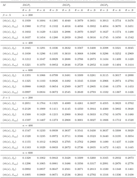
For the estimates ofm(x), we see that the one step backfitting method ˆm(x) dominates the pilot estimator
˜
m(x) across all data designs and sample sizes, using either estimate for . We notice that M actually decreases
as endogeneity increases almost everywhere, and in some cases this decrease is quite large. Like with the estimates for , the estimates ofm do not seem to be sensitive to the magnitude of , as M is consistent
across fixedDGPs and sample size, but varying values for .
Comparing across DGPs, DGP1 has consistently lower values for S and R than DGP2, which in turn
is lower than DGP3. For the estimate of m(x), DGP1 again is consistently easiest to estimate, where as
DGP3 has slightly smaller values compared to DGP2. Then, overallDGP1 is easiest to estimate for both
estimators of and both ofm.
Martins-Filho et al. (2015) showed that wp was consistent in the presence of endogeneity, and given
be used as a pilot estimator to construct a semiparametric efficient estimator for , a process discussed in Martins-Filho et al. (2015). Our results for ˆm(x) and ˜m(x) using wp and p supports the assertion that
ˆ
m(x) and ˜m(x) are oracle efficient and only a consistent estimator for is needed. There seems to be a
general trend that ˜m(x) preforms better with wpforDGP3, while inDGP1, DGP2it has a very slight edge
with p under the two higher levels of endogeneity. We do not observe this same kind of di↵erence with
ˆ
m(x).
From these results, we can conclude that these various estimators suitably account for the endogeneity of X, in general p out preforms wp in estimating , and ˆm(x) estimated with either estimate for
outperforms ˜m(x), and both ˆm(x) and ˜m(x) are relatively insensitive to the estimation method of used in
the calculations.
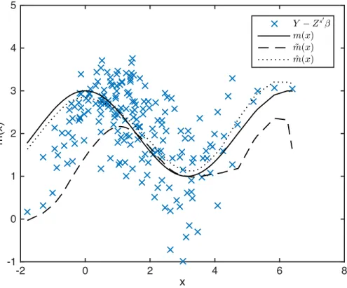
We include in figure demonstrating the estimators for the designDGP2, = 1,✓=.9 andn= 200. It is
visually evident that while both estimators match the curvature of the underlying structure, ˆm(x) provides
a much better goodness of fit.
6
Summary and Closing Remarks
In this paper we examine the derivation, computation, and asymptotic properties of a set of estimation procedures put forth by Martins-Filho et al. (2015), and test their finite sample performances with a Monte Carlo study. Under variousDGP designs, we conclude that the estimators sufficiently account for endogenous
variables entering the model nonparametrically, where the one step backfitting procedure and unweighted pilot estimators are more efficient in finite samples than their counterparts for estimating m(x) and
respectively.
In the same spirit, we could test estimators for alternative data structures than we had here. We could impose a di↵erent structure to the error, perhaps one which was conditionally heteroskedastic with or without stationarity similar to what was considered in Gao and Phillips (2013). Whatever the structure of the data, Monte Carlo studies will be perpetually useful in discerning the finite sample performance of various estimators, and will continue to be a mainstay in econometric literature, so there will always be work
of this nature to be done.
To expand the scope of this specific Monte Carlo study, we could examine the derivation of the semi-parametric efficient estimator for proposed in Martins-Filho et al. (2015) and compare the finite sample performance of an efficient estimator for to the others examined earlier in this paper. Alternatively, we could explicitly build on this work by examining the asymptotic properties of p to confirm that it is pn
consistent, and therefore suitable as the first stage in efficiently estimating , rather than just postulate this based on the finite sample properties.
References
Ai, C., Chen, X., 2003. Efficient estimation of models with conditional moment restrictions containing unknown functions. Econometrica 71, 1795–1843.
Gao, J., Phillips, P. C. B., 2013. Semiparametric estimation in triangular system equations with nonstation-arity. Journal of Econometrics 176, 59–79.
Martins-Filho, C., Yao, F., 2012. Kernel-based estimation of semiparametric regression in triangular systems. Economics Letters 115, 24–27.
Martins-Filho, C., Yao, F., Zhang, J., 2015. Efficient estimation of partially llinear models under nonpara-metric endogeneity, working paper.
Newey, W. K., Powell, J. L., Vella, F., 1999. Nonparametric estimation of triangular simultaneous equation models. Econometrica 67, 565–603.
Robinson, P. M., 1988. Root-n consistent semiparametric regression. Econometrica 56, 931–954.
Stone, C. J., 1982. Optimal rates of convergence for nonparametric regression. Annals of Statistics 10, 1040– 1053.
Stone, C. J., 1985. Additive regression and other nonparametric models. Annals of Statistics 13, 689–705. Su, L., 2008. Semi-parametric GMM estimation of spatial autoregressive models, working Paper.
7
Appendix - Tables and Figures
Table 1. Finite sample performance of estimates forDGP1
✓=.3 ✓=.6 ✓=.9 B S R B S R B S R =.5 n= 200 p -0.0039 0.2422 0.2421 -0.0105 0.2278 0.2279 0.0064 0.2235 0.2234 wp -0.0046 0.3456 0.3455 -0.0178 0.3732 0.3734 0.0237 0.4625 0.4629 n= 400 p -0.0027 0.1597 0.1596 0.0010 0.1722 0.1721 -0.0053 0.1397 0.1397 wp -0.0028 0.2516 0.2515 0.0121 0.3092 0.3093 -0.0086 0.2525 0.2525 n= 600 p 0.0000 0.1398 0.1397 -0.0001 0.1186 0.1185 -0.0023 0.1019 0.1019 wp -0.0003 0.2336 0.2335 -0.0049 0.2167 0.2167 -0.0071 0.2047 0.2047 = 1 n= 200 p -0.0109 0.2374 0.2375 0.0004 0.2301 0.2300 0.0094 0.2238 0.2239 wp -1.9472 0.3791 0.3794 0.0027 0.3432 0.3430 0.0059 0.5133 0.5131 n= 400 p -0.0018 0.1957 0.1956 -0.0109 0.1518 0.1521 -0.0014 0.1508 0.1507 wp -0.0030 0.3069 0.3067 -0.0129 0.2606 0.2608 0.0015 0.2692 0.2690 n= 600 p 0.0013 0.1460 0.1459 0.0036 0.1202 0.1202 -0.0005 0.1082 0.1081 wp 0.0031 0.2456 0.2455 0.0067 0.2273 0.2273 -0.0019 0.2234 0.2233
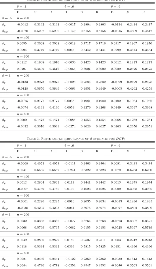
Table 2. Finite sample performance of estimates forDGP2 ✓=.3 ✓=.6 ✓=.9 B S R B S R B S R =.5 n= 200 p -0.0012 0.3162 0.3161 -0.0017 0.2804 0.2803 -0.0134 0.2414 0.2417 wp -0.0078 0.5232 0.5230 -0.0149 0.5156 0.5156 -0.0315 0.4609 0.4617 n= 400 p 0.0055 0.2008 0.2008 -0.0018 0.1717 0.1716 0.0117 0.1867 0.1870 wp 0.0094 0.3749 0.3749 0.0043 0.3442 0.3441 0.0299 0.3674 0.3684 n= 600 p 0.0112 0.1908 0.1910 -0.0030 0.1423 0.1423 0.0012 0.1213 0.1213 wp 0.0297 0.4609 0.4616 -0.0065 0.3001 0.3000 0.0029 0.2526 0.2525 = 1 n= 200 p -0.0133 0.2973 0.2975 -0.0025 0.2884 0.2882 -0.0029 0.2429 0.2428 wp -0.0128 0.5650 0.5649 -0.0063 0.4951 0.4949 -0.0005 0.4262 0.4259 n= 400 p -0.0075 0.2177 0.2177 0.0038 0.1981 0.1980 0.0102 0.1964 0.1966 wp -0.0074 0.4191 0.4190 0.0054 0.4270 0.4268 0.0149 0.3697 0.3698 n= 600 p 0.0000 0.1472 0.1471 -0.0085 0.1553 0.1554 0.0068 0.1262 0.1264 wp -0.0032 0.3070 0.3069 -0.0274 0.4020 0.4027 0.0103 0.2650 0.2651
Table 3. Finite sample performance of estimates forDGP3
✓=.3 ✓=.6 ✓=.9 B S R B S R B S R =.5 n= 200 p -0.0008 0.4053 0.4051 -0.0111 0.3463 0.3464 0.0091 0.3415 0.3414 wp 0.0041 0.6685 0.6682 -0.0241 0.6322 0.6323 0.0079 0.6283 0.6280 n= 400 p 0.0012 0.2804 0.2803 0.0112 0.2441 0.2442 0.0013 0.1975 0.1974 wp -0.0007 0.4789 0.4786 0.0195 0.4623 0.4625 0.0009 0.3968 0.3966 n= 600 p -0.0001 0.2226 0.2225 0.0016 0.2035 0.2034 -0.0013 0.1836 0.1835 wp -0.0038 0.4295 0.4293 0.0064 0.3975 0.3974 -0.0027 0.3802 0.3800 = 1 n= 200 p 0.0032 0.3368 0.3366 -0.0077 0.3764 0.3763 -0.0323 0.3307 0.3321 wp 0.0068 0.5799 0.5797 -0.0082 0.6155 0.6153 -0.0525 0.5697 0.5719 n= 400 p 0.0049 0.2830 0.2829 0.0159 0.2507 0.2511 0.0083 0.2242 0.2243 wp 0.0118 0.5334 0.5332 0.0399 0.5815 0.5825 0.0151 0.4396 0.4396 n= 600 p 0.0021 0.2456 0.2454 -0.0122 0.2360 0.2362 -0.0032 0.1643 0.1643 wp 0.0044 0.4720 0.4718 -0.0252 0.4547 0.4552 -0.0046 0.3503 0.3501
Table 4. Finite sample mean root mean square error (M) ofmestimators under all designs M DGP1 DGP2 DGP3 ✓=.3 ✓=.6 ✓=.9 ✓=.3 ✓=.6 ✓=.9 ✓=.3 ✓=.6 ✓=.9 =.5 n= 200 ( ˜m(x), p) 0.1939 0.1684 0.1385 0.4040 0.3979 0.3831 0.3913 0.3754 0.3476 ( ˜m(x), wp) 0.1980 0.1712 0.1532 0.4016 0.4056 0.3932 0.4054 0.3670 0.3451 ( ˆm(x), p) 0.1602 0.1429 0.1223 0.2896 0.2970 0.3027 0.1627 0.1574 0.1488 ( ˆm(x), wp) 0.1637 0.1454 0.1280 0.2859 0.2945 0.3016 0.1745 0.1650 0.1542 n= 400 ( ˜m(x), p) 0.1845 0.1291 0.1036 0.3632 0.3567 0.3400 0.3398 0.3321 0.3045 ( ˜m(x), wp) 0.1838 0.1296 0.1105 0.3610 0.3668 0.3496 0.3296 0.3252 0.2969 ( ˆm(x), p) 0.1212 0.1047 0.0829 0.2688 0.2766 0.2873 0.1434 0.1409 0.1420 ( ˆm(x), wp) 0.1221 0.1070 0.0852 0.2646 0.2728 0.2852 0.1449 0.1404 0.1414 n= 600 ( ˜m(x), p) 0.1355 0.1066 0.0799 0.3481 0.3309 0.3281 0.3115 0.3017 0.2890 ( ˜m(x), wp) 0.1325 0.1103 0.0826 0.3492 0.3345 0.3348 0.2966 0.2974 0.2794 ( ˆm(x), p) 0.0988 0.0825 0.0654 0.2569 0.2677 0.2805 0.1346 0.1370 0.1453 ( ˆm(x), wp) 0.0997 0.0834 0.0672 0.2545 0.2649 0.2793 0.1332 0.1367 0.1426 = 1 n= 200 ( ˜m(x), p) 0.2051 0.1764 0.1325 0.4089 0.4261 0.3837 0.4355 0.3823 0.3762 ( ˜m(x), wp) 0.2128 0.1909 0.1411 0.4145 0.4350 0.3944 0.4300 0.3802 0.3848 ( ˆm(x), p) 0.1568 0.1429 0.1215 0.2900 0.3043 0.3033 0.1792 0.1676 0.1480 ( ˆm(x), wp) 0.1597 0.1467 0.1273 0.2868 0.3001 0.3027 0.1806 0.1712 0.1520 n= 400 ( ˜m(x), p) 0.1547 0.1233 0.0939 0.3637 0.3541 0.3430 0.3637 0.3308 0.3029 ( ˜m(x), wp) 0.1520 0.1235 0.0972 0.3711 0.3586 0.3523 0.3440 0.3195 0.3054 ( ˆm(x), p) 0.1155 0.1012 0.0823 0.2705 0.2762 0.2860 0.1490 0.1437 0.1438 ( ˆm(x), wp) 0.1163 0.1029 0.0833 0.2672 0.2736 0.2835 0.1472 0.1421 0.1445 n= 600 ( ˜m(x), p) 0.1328 0.1062 0.0843 0.3428 0.3309 0.3260 0.3165 0.2932 0.2873 ( ˜m(x), wp) 0.1296 0.1065 0.0881 0.3486 0.3356 0.3317 0.2991 0.2876 0.2776 ( ˆm(x), p) 0.0992 0.0857 0.0647 0.2561 0.2671 0.2813 0.1330 0.1348 0.1461 ( ˆm(x), wp) 0.1005 0.0869 0.0671 0.2536 0.2641 0.2792 0.1316 0.1336 0.1438
x
-2 0 2 4 6 8m(x)
-1 0 1 2 3 4 5 Y !Zs0 -m(x) ~ m(x) ^ m(x)Figure 1: This is a plot of m(x) and the estimates using p under the design DGP2, = 1, ✓ = .9 and