http://dx.doi.org/10.12988/ams.2014.47548
Comparative Performance of ARIMA and
GARCH Models in Modelling and Forecasting
Volatility of Malaysia Market Properties and
Shares
Nor Hamizah Miswan1, Nor Azazi Ngatiman2, Khairum Hamzah3 and Zaminor Zamzamir Zamzamin4
1,2,3 Fakulti Teknologi Kejuruteraan
Universiti Teknikal Malaysia Melaka, Malaysia
4 Fakulti Keusahawanan dan Perniagaan
Universiti Malaysia Kelantan, Malaysia
Copyright © 2014 Nor Hamizah Miswan et al. This is an open access article distributed under the Creative Commons Attribution License, which permits unrestricted use, distribution, and reproduction in any medium, provided the original work is properly cited.
Abstract
Market properties and shares are important in the field of finance in order to measure the economic growth of a country. These market properties are volatile time series as they have huge price swings in a shortage or an oversupply period. In this study, we use two time series models which are Box-Jenkins Autoregressive Integrated Moving Average (ARIMA) and Generalized Autoregressive Conditional Heterocedasticity (GARCH) models in modelling and forecasting Malaysia property market. The capabilities of ARIMA and GARCH models in modelling and forecasting Malaysia property market will be evaluated by using Akaike's Information Criterion (AIC), Mean Absolute Percentage Error (MAPE) and Root Mean Squared Error (RMSE). It can be concluded that Box-Jenkins ARIMA model perform better compared than GARCH model in modelling and forecasting Malaysia market properties and shares.
Keywords: ARIMA, GARCH, Property, Share, Volatility
1 Introduction
The investment market is influenced by various economic conditions and factors. These factors not only affect the investment market internally but also affect the global investment. At times, the market is volatile with huge swings. Volatility is a condition where the conditional variance changes between extremely high and low values.
Malaysia has maintained its positive growth in gross domestic product (GDP) and expected to evolve in 2014 as a result of higher business and customer spending. The country is now still recovering from the epidemic that has resulted an increase of the unemployment rate. This has slightly affected the property sector as the terms and conditions become tighter and subsequently the borrowing for property purchasing has become too expensive. This crisis had a major impact to the overall financial markets including the property market and share.
Although Malaysia is one of the countries that can survive from both Asian and Global financial crisis, Malaysia should be more alert of the economic changes especially in the property investment sector since it is the largest contributor to GDP. In the current study, the volatility of the Malaysia Market Properties and Shares is investigated. The monthly data used are the Kuala Lumpur Stock Exchange Properties for properties and Kuala Lumpur Composite Index (KLCI) for shares from July 1997 to July 2012.
Two time series models where one has the ability to capture the non-constant volatility throughout the observations are used. These models are Autoregressive Integrated Moving Average (ARIMA) and Generalized Autoregressive Conditional Heterocedasticity (GARCH). These models will be used to fit the data where the best model will be used to forecast the future of forecasting market properties and shares.
2 Methodology
Data used for analysis using both ARIMA and GARCH models must be stationary. The data is said to be stationary if the mean, variance and autocorrelation structure are constant over the time interval. A stationary series
does not contain trend, it has no seasonality and flat looking. Stationarity of the data is important to describe the future behaviour of the process.
If the data are not stationary, we must transform them by using first difference. First differences are the data changes from one period to the next. Plotting the data of the first difference can reveal whether the data has been transformed to a stationary series or not. If it is still not stationary the second difference is taken. Model fitting can be carried out once the stationarity of the series has been achieved. In the current study, two time series models will be considered.
i) Box-Jenkins ARIMA models
Box-Jenkins ARIMA model has been used widely in many areas of Time Series analysis. Since ARIMA is among the earliest models, the capability of this model always being tested and widely used as a benchmark with other Time Series models. Box-Jenkins ARIMA is known as ARIMA(p,d,q) model where p is the number of autoregressive (AR) terms, d is the number of difference taken and
q is the number of moving average (MA) terms. ARIMA models always assume the variance of data to be constant. ARIMA(p,d,q) model can be represented by the following equation.
(1 − ∅1𝐵 − ⋯ − ∅𝑝𝐵𝑝)(1 − 𝐵)𝑑𝑌
𝑡 = 𝛿 + (1 − 𝜃1𝐵 − ⋯ − 𝜃𝑞𝐵𝑞)𝑎𝑡
where
1 − ∅1𝐵 − ∅2𝐵2− ⋯ − ∅
𝑝𝐵𝑝 is the AR operator of order 𝑝
1 − 𝜃1𝐵 − 𝜃2𝐵2− ⋯ − 𝜃
𝑞𝐵𝑞 is the MA operator of order 𝑞
𝛿 is the constant term
𝑎𝑡 is the shock element at time 𝑡
ii) GARCH models
GARCH model is known as a model of heterocedasticity which means not constant in variance. This model has been used widely in financial and business areas since the data of these areas tend to have variability or highly volatile throughout the time. GARCH model is written as GARCH(q,p) model where q is the number of moving average (MA) terms and p is the number of autoregressive (AR) terms. GARCH(q,p) model can be represented by the following equation.
𝑍𝑡 = 𝜇𝑡+ 𝜀𝑡 , 𝜀𝑡~𝑁(0, ℎ𝑡) 𝜀𝑡 = 𝑒𝑡√ℎ𝑡 , 𝑒𝑡~𝑁(0,1) ℎ𝑡= 𝛼 + ∑𝑝𝑖=1𝛽𝑖𝜀𝑡−𝑖2 + ∑ 𝛾 𝑖ℎ𝑡−𝑖 𝑞 𝑖=1 where
𝜇𝑡 is the mean or constant term
ℎ𝑡 is the conditional variance ℎ𝑡−𝑖 is the past conditional variance 𝜀𝑡−𝑖2 past squared residual return 𝛼 > 0, 𝛽𝑖 ≥ 0, 𝛾𝑖 ≥ 0
Before using any GARCH models, we need to check the volatility of a data. One of the methods is by computing histogram for a stationary series and check the distribution of data. Kurtosis is the measure of peakness of the data distribution and skewness is the measure of symmetrical of the distribution about the mean. When the value of kurtosis is greater than 3 and it is skewed either to the left or right, then the series is volatile. The kurtosis, K and skewness, S are defined as follows,
𝐾 =
1 𝑛.
∑𝑛𝑖=1(𝑦𝑖−𝑦̅)4 (𝑛1∑𝑛 (𝑦𝑖−𝑦̅)2 𝑖=1 ) 2𝑆 =
1𝑛.
∑𝑛𝑖=1(𝑦𝑖−𝑦̅)3 1 𝑛∑𝑛𝑖=1(𝑦𝑖−𝑦̅)3/2 where𝑦̅ is the mean of the data
𝑦𝑖 is the Time Series value of the data 𝑛 is the total number of observations
The first step in fitting the model is model identification. In order to determine the autoregressive (p) and moving average (q) values, correlogram of sample autocorrelation function (ACF) and partial autocorrelation function (PACF) will be computed. ACF and PACF specify the value of q and p respectively.
The next step is to estimate the parameters of the selected models by using Maximum Likelihood Estimation (MLE). MLE is suitable for both linear and nonlinear models and also satisfies all the properties of point estimator. MLE techniques will be applied to both ARIMA and GARCH models. The derivation of MLE for Box-Jenkins ARIMA model is given by the following equation.
𝑙 = −𝑛2ln{2𝜋𝜎𝑎2} −∑ 𝑎𝑡 2 𝑛 𝑡=1 2𝜎𝑎2 where
𝑙 is log-likelihood function of the distribution
𝑎𝑡 = 𝜃1𝑎𝑡−1+ ⋯ + 𝜃𝑞𝑎𝑡−𝑞+ 𝑌𝑡+ ∅1𝑌𝑡−1− ⋯ − ∅𝑝𝑌𝑡−𝑝
𝜎̂𝑎2 =
∑𝑛 𝑎𝑡2 𝑡=𝑝+1
df , df = n − (2p + q + 1)
The derivation of MLE for GARCH model is defined as follows,
𝑙 == −𝑛2ln{2𝜋} −12∑ {ln{ℎ𝑡} +𝑒𝑡2 ℎ𝑡} 𝑛
𝑡=1 (7)
where
𝑙 is log-likelihood function of the distribution ℎ𝑡 = 𝛼 + ∑ 𝛽𝑖 𝑝 𝑖=1 𝜀𝑡−𝑖2 + ∑ 𝛾 𝑖ℎ𝑡−𝑖 𝑞 𝑖=1
To select the best model fitting, Akaike Information Criterion (AIC) can be used. The smaller the value of AIC, the better is the model fitting. AIC is defined as follows,
𝐴𝐼𝐶 = 𝑛 ln(𝑀𝑆𝐸) − 𝑛 ln 𝑛 + 2𝑝 where
𝑝 is the number of parameters used 𝑛 is the number of observations
𝑀𝑆𝐸 is Mean Square Error of the model
The next step is forecasting. The purpose of forecasting is to predict the future values of the data. The accuracy of the forecasting model can be evaluated by computing the forecast accuracy criterion. Accuracy can be measured using Mean Absolute Percentage Error (MAPE) and Root Mean Square Error (RMSE) and it is defined as,
𝑀𝐴𝑃𝐸 = {[∑ |𝑦𝑡−𝑦̂𝑡 𝑦𝑡 | 𝑛
𝑅𝑀𝑆𝐸 = √{∑𝑛𝑡=1(𝑦𝑡−𝑦̂𝑡)2} 𝑛⁄
where
𝑦𝑡 is the actual value
𝑦̂𝑡 is the forecast value
n is the number of period.
The smaller the values of MAPE and RMSE, the better are the model.
3 Data Analysis and Results
Data of Kuala Lumpur Stock Kuala Lumpur Stock Exchange Properties and Kuala Lumpur Composite Index (KLCI) are plotted in Figure 1 and Figure 2.
Figure 1 : Kuala Lumpur Stock Exchange Properties from July 1997 to July 2012
Figure 2 : Kuala Lumpur Composite Index (KLCI) from July 1997 to July 2012
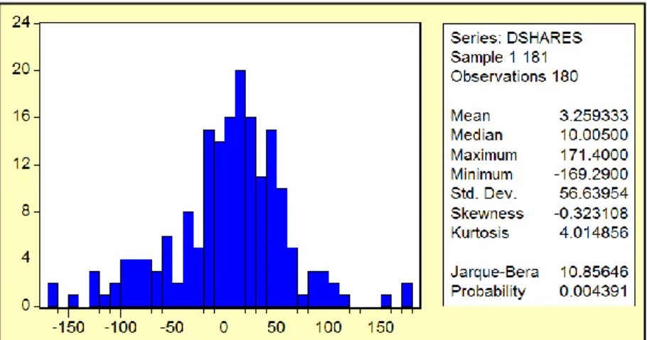
For both observations, it is clear that both data are not stationary. Hence, first difference of the data is needed. For GARCH models, we need to plot the histogram at first difference level. GARCH can only be used when the data is volatile. Figure 3 and Figure 4 show the histogram and descriptive statistics for both data at first difference level.
Figure 3 : Histogram for Kuala Lumpur Stock Exchange Properties at first difference level
Figure 4 : Histogram for Kuala Lumpur Composite Index (KLCI) at first difference level
The values of kurtosis for both series are more than 3 and skewed to the left indicating that GARCH models can be used for both series. Next, identifying the models involved can be done by computing the sample PACF, p and ACF, q. ARIMA model is denoted by ARIMA(p,d,q) and GARCH(q,p) for GARCH model. The order of differencing, d is 1 since we are taking first difference of the series.
The corresponding value of p is 1 and values of q are 1 and 4 for properties data and for shares, the values of p and q are both 1 and 7. In order to obtain the parameters values for each models, Eviews software are used. Table 1, Table 2, Table 3 and Table 4 show the equation of ARIMA(p,d,q) and GARCH(q,p) and their corresponding AIC values.
Table 1 : Equation of ARIMA(p,d,q) models for Kuala Lumpur Stock Exchange Properties and their corresponding AIC values
Model Equation AIC
ARIMA(1,1,1) (1 − 0.769497𝐵)(1 − 𝐵)𝑦 𝑡 = 3.002597 + (1 + 0.753951𝐵)𝑎𝑡 11.55521 ARIMA(1,1,4) (1 − 0.818696𝐵)(1 − 𝐵)𝑦 𝑡 = −1.644376 + (1 + 0.576091𝐵 + 0.375584𝐵2− 0.077890𝐵3 + 0.244720𝐵4)𝑎 𝑡 11.39220 ARIMA(1,1,0) (1 − 0.360012𝐵)(1 − 𝐵)𝑦 𝑡 = −3.820079 + 𝑎𝑡 11.61201 ARIMA(0,1,1) (1 − 𝐵)𝑦 𝑡 = −6.462743 + (1 − 0.432535𝐵)𝑎𝑡 11.64870 ARIMA(0,1,4) (1 − 𝐵)𝑦 𝑡= −6.502618 + (1 − 0.433552𝐵 − 0.094861𝐵2 −0.225968𝐵3+ 0.017799𝐵4)𝑎 𝑡 11.63985
Table 2 : Conditional variance equation of GARCH(q,p) models for Kuala Lumpur Stock Exchange Properties and their corresponding AIC values
Model Equation AIC
GARCH(1,1) ℎ𝑡2= 226.2584 + 0.159873𝜀𝑡−12 + 0.763929ℎ𝑡−12 11.17227 GARCH(4,1) ℎ𝑡2= 438.5962 + 0.350611𝜀𝑡−12 1.158576ℎ𝑡−12 − 1.164714ℎ𝑡−22 +0.774968ℎ𝑡−32 − 0.174557ℎ𝑡−42 11.14682 ARCH(1) ℎ𝑡2= 3886.305 + 0.432588𝜀𝑡−12 11.53150
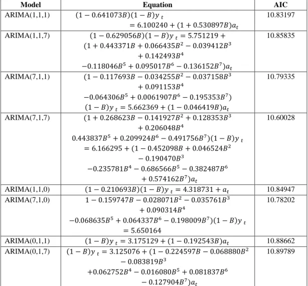
Table 3 : Equation of ARIMA(p,d,q) models for Kuala Lumpur Composite Index (KLCI) and their corresponding AIC values
Model Equation AIC
ARIMA(1,1,1) (1 − 0.641073𝐵)(1 − 𝐵)𝑦 𝑡 = 6.100240 + (1 + 0.530897𝐵)𝑎𝑡 10.83197 ARIMA(1,1,7) (1 − 0.629056𝐵)(1 − 𝐵)𝑦 𝑡= 5.751219 + (1 + 0.443371𝐵 + 0.066435𝐵2− 0.039412𝐵3 + 0.142493𝐵4 −0.118046𝐵5+ 0.095017𝐵6− 0.136152𝐵7)𝑎 𝑡 10.85835 ARIMA(7,1,1) (1 − 0.117693𝐵 − 0.034255𝐵2− 0.037158𝐵3 + 0.091153𝐵4 −0.064306𝐵5+ 0.0061907𝐵6− 0.195353𝐵7) (1 − 𝐵)𝑦 𝑡= 5.662369 + (1 − 0.046419𝐵)𝑎𝑡 10.79335 ARIMA(7,1,7) (1 + 0.268623𝐵 − 0.141927𝐵2+ 0.128353𝐵3 + 0.206048𝐵4 0.443837𝐵5+ 0.209924𝐵6− 0.491756𝐵7)(1 − 𝐵)𝑦 𝑡 = 6.166295 + (1 − 0.452098𝐵 + 0.046524𝐵2 − 0.190470𝐵3 −0.235781𝐵4− 0.686566𝐵5− 0.382487𝐵6 + 0.574162𝐵7)𝑎 𝑡 10.60028 ARIMA(1,1,0) (1 − 0.210693𝐵)(1 − 𝐵)𝑦 𝑡= 4.318731 + 𝑎𝑡 10.84947 ARIMA(7,1,0) 1 − 0.159747𝐵 − 0.028071𝐵2− 0.035761𝐵3 + 0.090314𝐵4 −0.068635𝐵5+ 0.064337𝐵6− 0.198009𝐵7)(1 − 𝐵)𝑦 𝑡 = 5.650164 10.78202 ARIMA(0,1,1) (1 − 𝐵)𝑦 𝑡= 3.175129 + (1 − 0.192543𝐵)𝑎𝑡 10.88662 ARIMA(0,1,7) (1 − 𝐵)𝑦 𝑡= 3.125076 + (1 − 0.224597𝐵 − 0.068880𝐵2 − 0.083819𝐵3 +0.062752𝐵4− 0.016080𝐵5+ 0.081837𝐵6 − 0.127904𝐵7)𝑎 𝑡 10.89789
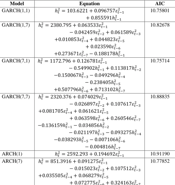
Table 4 : Conditional variance equation of GARCH(q,p) models for Kuala Lumpur Composite Index (KLCI) and their corresponding AIC values
Model Equation AIC
GARCH(1,1) ℎ𝑡2 = 103.6221 + 0.096757𝜀𝑡−12 + 0.855591ℎ𝑡−12 10.75801 GARCH(1,7) ℎ𝑡2 = 2380.795 + 0.063533𝜀𝑡−12 − 0.042459𝜀𝑡−22 + 0.061589𝜀 𝑡−32 +0.010853𝜀𝑡−42 + 0.044823𝜀𝑡−52 + 0.023590𝜀𝑡−62 +0.273671𝜀𝑡−72 − 0.188178ℎ 𝑡−1 2 10.82678 GARCH(7,1) ℎ𝑡2 = 1172.796 + 0.126781𝜀𝑡−12 − 0.549902ℎ𝑡−12 + 0.113817ℎ 𝑡−2 2 −0.150067ℎ𝑡−32 − 0.049296ℎ 𝑡−4 2 − 0.238405ℎ𝑡−52 +0.507796ℎ𝑡−62 + 0.713102ℎ 𝑡−7 2 10.75714 GARCH(7,7) ℎ𝑡2 = 2320.376 + 0.074029𝜀𝑡−12 − 0.026897𝜀𝑡−22 + 0.107617𝜀 𝑡−32 +0.081705𝜀𝑡−42 + 0.061621𝜀𝑡−52 + 0.063598𝜀𝑡−62 + 0.260546𝜀 𝑡−72 −0.136159ℎ𝑡−12 − 0.034856ℎ 𝑡−2 2 − 0.021197ℎ𝑡−32 − 0.093275ℎ 𝑡−4 2 −0.038293ℎ𝑡−52 − 0.007106ℎ 𝑡−6 2 − 0.004816ℎ𝑡−72 10.88835 ARCH(1) ℎ𝑡2 = 2592.293 + 0.194692𝜀𝑡−12 10.91190 ARCH(7) ℎ𝑡2 = 851.3916 + 0.091275𝜀𝑡−12 − 0.015023𝜀𝑡−22 + 0.107512𝜀 𝑡−32 +0.035505𝜀𝑡−42 + 0.068279𝜀𝑡−52 + 0.072775𝜀𝑡−62 + 0.324163𝜀 𝑡−72 10.77852
From the above tables, the lowest AIC values are considered to be the best model for modelling properties and shares data. Hence, it can be concluded that ARIMA(1,1,4) and GARCH(4,1) are the best model for Kuala Lumpur Stock Exchange Properties where the AIC values are 11.39220 and 11.14682 respectively. For KLCI series, ARIMA(7,1,7) and GARCH(7,1) are the best models where the AIC values are 10.60028 and 10.75714.
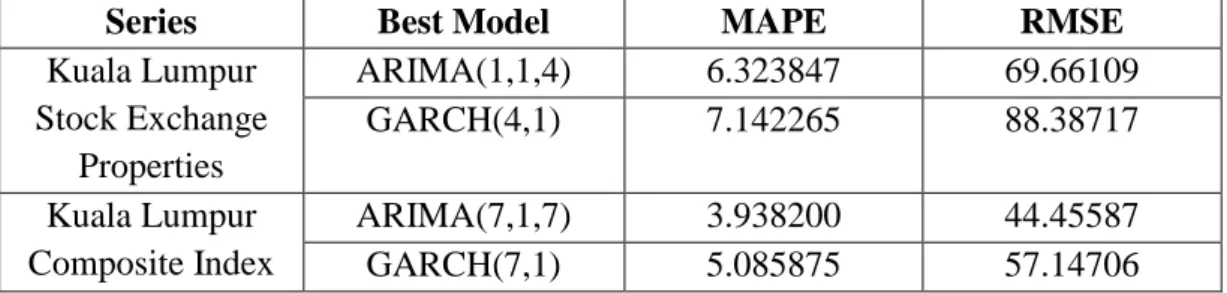
The best models will be used to forecast the data and check the accuracy of these models by using forecast accuracy criterion, MAPE and RMSE. The lowest MAPE and RMSE values are considered to best the best model for forecasting properties and shares data. Table 5 tabulates the MAPE and RMSE values when the selected models
Table 5 : Forecasting performances of ARIMA and GARCH models
Series Best Model MAPE RMSE
Kuala Lumpur Stock Exchange Properties ARIMA(1,1,4) 6.323847 69.66109 GARCH(4,1) 7.142265 88.38717 Kuala Lumpur Composite Index ARIMA(7,1,7) 3.938200 44.45587 GARCH(7,1) 5.085875 57.14706
From Table 5, the MAPE and RMSE values for ARIMA(1,1,4) are smaller for Kuala Lumpur Stock Exchange Properties and ARIMA(7,1,7) are smaller for Kuala Lumpur Composite Index data. The differences in MAPE and RMSE values between ARIMA and GARCH models for properties data are 0.818418 and 18.72608 and for shares data are 1.147675 and 12.69119. These differences are considered large.
4 Conclusion
It is known that GARCH models have been used widely for volatile data. However, for Kuala Lumpur Stock Exchange Properties and Kuala Lumpur Composite Index, GARCH models cannot give the best result. One of the reason is the data are not highly volatile based on the values of kurtosis which are only 6.716612 and 4.014856. Hence, GARCH models cannot capture variability of the data much better that ARIMA models.
As a conclusion, ARIMA is the best models in modelling and forecasting Malaysia market properties and shares as compared to GARCH model. Hence, ARIMA model can be used to predict the future values of Malaysia properties and shares. The forecasting values can help firm and investors to plan their market strategy as well as bring Malaysia economic towards positive growth.
Acknowledgements. The main author would like to acknowledge the support of the Faculty of Engineering Technology (FTK), Universiti Teknikal Malaysia Melaka (UTeM).
References
[1] D.H. Ackley, G.E. Hinton and T.J. Sejnowski, A learning algorithm for Boltzmann machine, Cognitive Science, 9 (1985), 147 - 169.
[2] F.L. Crane, H. Low, P. Navas, I.L. Sun, Control of cell growth by plasma membrane NADH oxidation, Pure and Applied Chemical Sciences, 1 (2013), 31 - 42. http://dx.doi.org/10.12988/pacs.2013.3310
[3] D.O. Hebb, The Organization of Behavior, Wiley, New York, 1949.
[4] Chong Choo, Nie Lee and Nie Ung, Macroeconomics Uncertainty and Performance of GARCH Models in Forecasting Japan Stock Market Volatility.
International Journal of Business and Social Science, 2 (2011), 200-208 (2011) [5] J. D. Cryer and K. S. Chan, Time Series Analysis with Applications in R (2nd ed.), New York : Springer, 2008
[6] Malaysia GDP to Grow 5.1% in 2013, 2014 : World Bank (2013)[Online]. Accessed [6th January 2014]. Available from The Sun Daily : www.the sundaily.my/news/751900
[7] Nor Hamizah Miswan, Modelling and Forecasting Volatile Data by using ARIMA and GARCH Models, Master Thesis, Universiti Teknologi Malaysia, 2013.
[8] Pung Yean Ping, Nor Hamizah Miswan and Maizah Hura Ahmad, Forecasting Malaysian Gold using GARCH Model, Applied Mathematical Sciences, 7 (2013), 2879-2884