Damoulas, Theodoros (2009)
Probabilistic multiple kernel learning.
PhD thesis.
https://theses.gla.ac.uk/1266/
Copyright and moral rights for this work are retained by the author
A copy can be downloaded for personal non-commercial research or study,
without prior permission or charge
This work cannot be reproduced or quoted extensively from without first
obtaining permission in writing from the author
The content must not be changed in any way or sold commercially in any
format or medium without the formal permission of the author
When referring to this work, full bibliographic details including the author,
title, awarding institution and date of the thesis must be given
Enlighten: Theses
https://theses.gla.ac.uk/ [email protected]
by
Theodoros Damoulas
A dissertation submitted to
The Department of Computing Science
of
The University of Glasgow
for the degree of
Doctor of Philosophy
October 2009
Abstract
The integration of multiple and possibly heterogeneous information sources for an overall decision-making process has been an open and unresolved research direction in computing science since its very beginning. This thesis attempts to address parts of that direction by proposing probabilistic data integration algorithms for multiclass decisions where an observation of interest is assigned to one of many categories based on aplurality of information channels.
Motivation for this thesis, from an application perspective, comes from the Automatic Currency Validation setting where the problem is to automatically classify currency notes, deposited in an Automated Teller Machine, to one of multiple classes while utilising information from multiple sensors. The adopted Bayesian probabilistic framework is motivated by the requirements for assessing decision-making costs, formal inclusion of prior knowledge and principled model selection. Requirements that are common across many fields, such as bioinfor-matics and robotics, where multiple sources of information are available for a multiclass classification decision.
There is a single light of science, and to brighten it anywhere is to brighten it everywhere.
Acknowledgements
This thesis would not have been possible without the help and support of many people, to only some of whom it is possible to give mention and acknowl-edge here.
First of all I would like to thank my supervisor Prof. Mark Girolami for his guidance and support, for giving me directions and keeping me on track, and for his patience and understanding. Furthermore, I would like to thank him for giving me the opportunity to apply for the RAEng fellowship which taught me other aspects of research and academia and also to acknowledge the additional funding for the write up months that he provided. Thank you for everything Mark, I hope to make you proud in the future.
I was very lucky to also have the guiding hand of “Uncle Keith”, my second supervisor Prof. C. J. Keith van Rijsbergen. I would like to thank him for being a role model for me, for giving me the appropriate hard time on my yearly progression examinations and for introducing me to the gems of I. J. Good and Bruno de Finetti.
Dr. Simon Rogers also had a significant impact on this thesis and my de-velopment through numerous discussions on Multiple Kernel Learning, support and direct feedback in many levels including corrections on drafts of this thesis and on my fellowship. I would like to thank him for also being a good friend throughout these years.
During this period I had the pleasure to collaborate with Dr. Colin Campbell and Dr. Yiming Ying from the University of Bristol. I would like to thank them for the numerous discussions and great time we had while developing some of the algorithms in this thesis.
This thesis was funded by NCR Financial Solutions Ltd and I benefited from interaction with research engineers from the NCR Labs. I would like to thank especially Dr. Chao He and Dr. Gary Ross for their help, support and for providing the necessary datasets and currency images.
Furthermore, thanks are due to the whole of the Inference Research Group and people from the Information Retrieval Group for their friendship, company and help. In particular, Ben, Billy, Dom, Iraklis, Keith, Tamara and Vlad (alphabetical order) helped me with research matters such as ESS scripts, the-sis templates, programming, statistical advice, scientific discussions and coffee (beer) breaks. During the last year I had the pleasure of supervising the MSc
IT thesis of Yannis Psorakis and some of our work is included in this thesis. It is always a joy to interact with a great student and also gain a friend in the process.
On the final research side of things, I would like to thank my external and internal examiners Dr. Guido Sanguinetti and Dr. Paul Siebert for agreeing to read my thesis in due time and hence help me to a smoother transition from Glasgow to Cornell University while meeting the requirements and deadlines.
On a more personal and less technical note, I had the luck of being sur-rounded with people that supported me intellectually, emotionally and finan-cially through these times. I owe a big thank you to my “extended” family (Damouleiko, Spaneiko, Tsakireiko) and my friends from back home (P.Club) and abroad. Special thanks to Vassiliki Grammenou for providing coffee and helping me during the correction phase. I also had the pleasure of meeting some new people this period that I would like to thank for their friendship and backing, especially Prof. Christos Papatheodorou and Periklis Vandoros. Finally, during the last year I was very lucky to have the attention and care of a lovely girl called Tamara Polajnar who has also helped me a lot in many ways, including help in binding and submitting this thesis.
Dedicated to my mother Ioanna Tsakiri
Declaration
All the work reported in this thesis has been performed by myself, unless specifically stated otherwise.
Theodoros Damoulas
Notation
Symbols
RD Real D - dimensional space.
RDs The real Ds - dimensional space of information source s∈ {1, . . . , S}.
RN×D Real N ×D - dimensional space.
N The set of natural numbers (positive integers).
x Scalar ∈R.
x Column vector ∈RD.
X Matrix ∈RN×D.
x(s) Column vector x∈
RDs from thesth information source. wc The cth column vector of matrix1 W∈RN×C.
xα x raised to theα power.
x∗ An “unseen” or new x.
p(z) Probability density function (p.d.f) of z.
p(z|y) Conditional p.d.f of z given y.
p(z,y) Joint p.d.f of z and y.
z∼p(z) z is distributed according to p(z).
O(N) The computational complexity is order N operations.
Operators and functions
AT Transpose of matrix A.
A−1 Inverse of matrixA.
Tr [A] Trace of matrixA.
|A| Determinant of matrixA.
δi Dirac delta function (impulse function).
Ep(z)(z) Expectation of the random variable z wrt. p(z). exp(·) Exponential function.
log(·) Naperian logarithmic function (ln). min,max Extrema with respect to an integer value. argmax
x
The argumentx that maximizes the operand. argmin
x
The argumentx that minimizes the operand. 1To simplify the notation we denotew
cas an equivalent toW1:N,cand as anNdimensional
column vector. That is, every vectorial representation will be denoted by lower-case bold (vice versa) and if an index is not appearing we are referring to all of its possible values. All vectors are column vectors.
Standard probability distributions Binomial Bk(n, p) nk pk(1−p)n−k Dirichlet Dx(ρ) Γ(PS i=1ρi) QS i=1Γ(ρi) QS i=1x ρi−1 i with x,ρ∈RS Exponential Ex(λ) λexp(−λx) Gamma Gx(α, β) β α Γ(α)x α−1exp(−βx) Gaussian Nx(µ,Σ) |2πΣ|−1/2exp −1 2(x−µ) T Σ−1(x−µ) with x,µ∈RN and Σ∈ RN×N
Inverse Gamma IG(α, β) Γ(βαα)x−α−1exp(−β/x)
Abbreviations
ANN Artificial Neural Network.
ARD Automatic Relevance Determination.
CDF Cumulative Distribution Function.
CPU Central Processing Unit.
EM Expectation Maximisation.
GLM Generalized Linear Model.
GP Gaussian Process.
i.i.d Independent and Identically Distributed.
IVM Informative Vector Machine.
KLD Kullback Leibler Divergence.
MAP Maximum A Posteriori.
MCMC Markov Chain Monte Carlo.
MH Metropolis Hastings.
MKL Multiple Kernel Learning.
ML Maximum Likelihood.
p.d.f Probability Density Function. p.s.d Positive Semi-Definite.
QP Quadratic Programming.
RBF Radial Basis Function.
RVM Relevance Vector Machine.
SVM Support Vector Machine.
Terminology
x Input sample, input variable, predictor, regressor.
1 Introduction 22
1.1 Learning from Multiple Sources . . . 22
1.2 Contributions . . . 23
1.3 Thought Process . . . 25
1.4 Thesis Structure . . . 26
2 Introduction to Multiple Kernel Learning 27 2.1 Linear Regression and Nonlinear Responses . . . 28
2.2 Learning and Bayesian Inference . . . 30
2.2.1 Statistical Learning Theory . . . 30
2.2.2 Towards Bayesian Inference . . . 32
2.2.3 Bayesian Inference . . . 33
2.3 The Kernel Trick and Kernel Regression . . . 36
2.4 Classification . . . 39
2.4.1 Logistic and Probit Regression . . . 40
2.5 Markov Chain Monte Carlo . . . 41
2.5.1 Importance Sampling . . . 42
2.5.2 Metropolis Sampling . . . 44
2.5.3 Metropolis-Hastings Sampling . . . 44
2.5.4 Gibbs Sampling . . . 45
2.6 Deterministic Approximations . . . 46
2.6.1 Saddle-point (Laplace) Approximation . . . 46
2.6.2 Variational Free Energy Minimisation . . . 52
2.7 Sparsity and Shrinkage methods . . . 54
2.7.1 Ridge Regression and the Lasso . . . 55
2.7.2 Sparsity in Kernel Methods . . . 56
2.7.3 Sparsity in Bayesian Inference . . . 56
2.8 Ensemble Learning . . . 58
2.8.1 Classifier Combination . . . 59
2.8.2 Multiple Kernel Learning . . . 61
3 Probabilistic Multiple Kernel Learning 67 3.1 Introduction . . . 67
3.2 Constructing the Composite Kernel . . . 67
3.2.1 Fixed Combination . . . 68
3.2.2 Convex Linear Combination . . . 68
3.2.3 Binary Combination . . . 69
3.2.4 Product Combination . . . 69
3.2.5 Weighted Product Combination . . . 69
3.2.6 Theoretical Justification of Kernel Combinations . . . 70
3.3 Multinomial Probit Kernel Regression . . . 70
3.3.1 Multinomial Probit Likelihood . . . 71
3.3.2 Gauss-Hermite Quadrature . . . 73
3.3.3 Prior distributions and the graphical model . . . 73
3.4 Markov Chain Monte Carlo Posterior Inference . . . 77
3.4.1 Gibbs Sampler . . . 77
3.4.2 Metropolis Hastings Sampler . . . 80
3.5 Marginal Likelihood for Model Selection . . . 82
3.6 Comparison of MCMC Sampling Schemes . . . 83
3.7 Toy Example Demonstration . . . 86
3.8 Computational Complexity . . . 87
3.9 Discussion . . . 87
4 Variational Bayes Inference 90 4.1 Mean Field Theory . . . 91
4.1.1 Variational Mean Field Theory for Classification . . . 91
4.2 Variational Bayes Probabilistic Multiple Kernel Learning . . . 93
4.2.1 Q(Y): Approximate posterior for Y . . . 95
4.2.2 Q(W): Approximate posterior for regression coefficients W 96 4.2.3 Q(A): Approximate posterior of scales A. . . 97
4.2.4 Q(Θ): Approximate posterior for Θ . . . 98
4.2.6 Q(ρ)Q(π)Q(χ): Approximate posteriors for ρ,π,χ . . . 99
4.2.7 Predictive Distribution . . . 100
4.3 Convergence and the Lower Bound . . . 101
4.4 Computational Complexity . . . 102
4.5 Variational Inference and Gibbs Sampling . . . 103
4.5.1 Synthetic Data sets . . . 103
4.6 Multinomial UCI Experiments . . . 107
4.7 Discussion . . . 108
5 MAP Estimators and mRVMs 110 5.1 MAP Estimation and EM Update Schemes . . . 111
5.2 Sparsity and Relevance Vector Machines . . . 114
5.3 Multiclass Multi-kernel Relevance Vector Machines . . . 115
5.4 Model Formulation . . . 116
5.4.1 mRVM1 . . . 117
5.4.2 Computational Efficiency for mRVM1 . . . 120
5.4.3 Informative Sample Selection for mRVM1 . . . 121
5.4.4 Initialisation and Convergence for mRVM1 . . . 123
5.4.5 mRVM2 . . . 125
5.4.6 Initialisation and Convergence Criteria for mRVM2 . . . . 126
5.5 Preliminary Experimental Evaluation . . . 126
5.5.1 Experimental Setup . . . 127
5.5.2 Non-sparse Comparison . . . 127
5.5.3 Sparse Comparison . . . 128
5.5.4 Convergence, Sparsity and Predictive Power . . . 129
5.6 Discussion . . . 138
6 Automatic Currency Validation 140 6.1 Motivation . . . 140
6.2 ACV Literature Review . . . 142
6.2.1 Recognition and Verification of Currency . . . 142
6.3 ACV with Multiple Sources of Information . . . 148
6.4 Feature Extraction . . . 150
6.4.1 Image Channels . . . 150
6.4.2 Non-Image Channels . . . 151
6.5.1 Binary Classification . . . 152
6.5.2 Multinomial Classification . . . 156
6.6 VBpMKL Results . . . 157
6.6.1 Image Integration . . . 158
6.6.2 Image and Non-Image Integration . . . 163
6.7 mRVM Results . . . 167
6.8 Discussion . . . 171
7 Further Large Scale Applications 173 7.1 Handwritten Numeral Recognition . . . 174
7.1.1 Multiple Features Dataset: Gibbs Sampling . . . 175
7.1.2 Multiple Features Dataset: Variational Bayes . . . 180
7.2 Protein Fold Recognition . . . 182
7.2.1 Experimental Setup . . . 184
7.2.2 Results and Discussion . . . 186
7.3 Remote Homology Detection . . . 190
7.4 Protein Subcellular Localisation . . . 191
7.5 Discussion . . . 194
8 Diversity in Multiple Kernel Learning 196 8.1 The Flat Maximum Effect . . . 197
8.1.1 Linear regression model . . . 197
8.1.2 Extension to Multiple Kernel Learning . . . 199
8.2 The Ambiguity Decomposition . . . 200
8.3 Bias-Variance-Covariance Decomposition . . . 201
8.4 Diversity and Information . . . 203
8.5 Fisher Information for MKL . . . 205
8.5.1 Fisher Information of β . . . 206
8.5.2 Fisher Information of the regression coefficients w . . . 206
8.5.3 Maximisation of the Fisher Information . . . 207
8.6 Discussion . . . 209
9 Conclusions and Future Research Directions 210 9.1 Future Research Directions . . . 212
A Posterior Inference in MCMC 214
A.1 Kernel Combination Parameters . . . 214
A.1.1 Convex Linear Combination . . . 214
A.1.2 Weighted Product Combination . . . 214
A.1.3 Binary Combination . . . 215
A.2 Kernel Parameters . . . 216
B Variational Approximations 217 B.1 Approximate posterior distributions . . . 217
B.1.1 Q(Y) . . . 217
B.1.2 Q(W) . . . 218
B.1.3 Q(A) . . . 219
B.1.4 Q(β), Q(ρ), Q(Θ) . . . 219
B.2 Posterior Expectations for the Auxiliary Variables . . . 221
B.3 Predictive distribution . . . 222
B.4 Lower bound . . . 224
2.1 The supervised learning setting. . . 31
2.2 The intuition behind Multiple Kernel Learning and the differences with Classifier Combination methods. . . 62
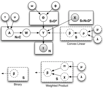
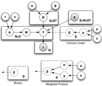
3.1 Plates diagram of the model depicting the conditional relation-ships of model variables together with the dimensionality of cor-responding plates. The dotted plates depict variations for the three parametric combination rules. . . 74
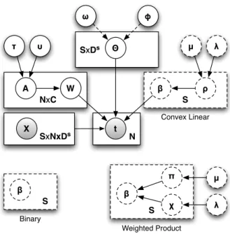
3.2 Plates diagram of the reduced model depicting the conditional relationships of model variables together with the dimensionality of corresponding plates. The dotted plates depict variations for the three parametric combination rules. . . 81
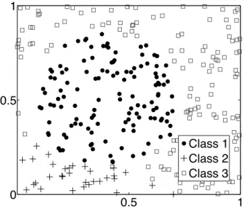
3.3 The artificial dataset. . . 84
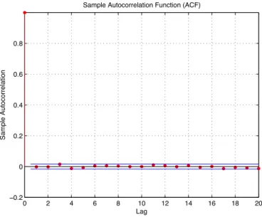
3.4 Typical Autocorrelation from the Gibbs sampler. . . 85
3.5 Typical Autocorrelation from the Metropolis sampler. . . 86
3.6 Three combined sources with varying informational content. No-tice how the the original informative kernel receives 80% of the weight, with the partially informative kernel receiving the rest 20% and the non-informative kernel being effectively discarded. . 87
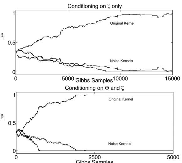
3.7 The effect of conditioning on the Neal dataset. As the param-eter space expands, the required steps of the Gibbs sampler for convergence increase. . . 88
3.8 Inferring θi and hence learning the importance of the features. The uninformative features, as it can be seen, receive a very low weight and are effectively discarded. . . 88
4.1 Plates diagram of the model depicting the conditional relation-ships of model variables together with the dimensionality of cor-responding plates. The dotted plates depict variations for the
three parametric combination rules. . . 94
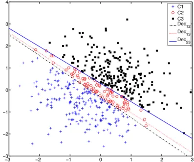
4.2 Linearly separable dataset with known regression coefficients defin-ing the decision boundaries. Cn denotes the members of class n and Decij is the decision boundary between classes i and j. . . 104
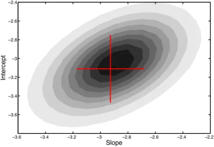
4.3 Gibbs posterior distribution of a decision boundary’s (Dec12) slope and intercept for a Markov chain of 100,000 samples. The cross describes the original decision boundary employed to sample the dataset. . . 105
4.4 The variational approximate posterior distribution for the same case as above. Employing 100,000 samples from the approximate posterior of the regression coefficientsW in order to estimate the approximate posterior of the slope and intercept. . . 105
4.5 Decision boundaries from the Gibbs sampling solution on Neal’s dataset. . . 106
4.6 Decision boundaries from the variational approximation on Neal’s dataset. . . 107
5.1 Plates diagram of the model. . . 117
5.2 Neal dataset. Left: Uninformative sample selection. Right: in-formative sample selection . . . 123
5.3 Top: Random Initialisation ofY and 50 cases that initialise con-trary to the labels and probit link relation. Bottom: Aligned Initialisation of Y and 50 randomly selected cases (all follow the target labels from the start). . . 124
5.4 Typical Relevance vectors . . . 128
5.5 Balance dataset. Top: mRVM1 Bottom: mRVM2 . . . 131
5.6 Glass dataset. Top: mRVM1 Bottom: mRVM2 . . . 132
5.7 Iris dataset. Top: mRVM1 Bottom: mRVM2 . . . 133
5.8 Soybean dataset. Top: mRVM1 Bottom: mRVM2 . . . 134
5.9 Vehicle dataset. Top: mRVM1 Bottom: mRVM2 . . . 135
6.1 Multiple Sources of Automated Currency Validation. The de-posited currency note produces crude sensory information from which features are extracted and later combined via the proposed pMKL methodology towards a final classification decision. Images not necessarily representative of sensor measurements. . . 149 6.2 Typical extraction masks for some Image channels. . . 151 6.3 Typical Markov chain from the GLMs. Top: Acceptance ratio
tuned to 30%. Bottom: Samples from the regression coefficients posterior distribution. . . 153 6.4 Some posterior distributions (smoothened via a Parzen window
type filter) from the Markov chain. Top row: Posteriors signif-icantly deviating from the zero-mean prior. Bottom: Posteriors not deviating from the zero-mean prior. . . 153 6.5 Typical Z-scores for the binary classification between genuine and
counterfeit notes. . . 154 6.6 Typical error progression with the logistic regression models. . . . 155 6.7 Typical error progression with the probit regression models. . . . 155 6.8 Typical Z-scores for the multiclass classification between genuine
new, genuine old and counterfeit notes. . . 156 6.9 Typical error progression on the multiclass ACV case. . . 157 6.10 Learning curves on $50 currency notes. . . 159 6.11 Predictive likelihood progressions for varying training size on $50. 159 6.12 CPU time requirements for varying training size on $50. . . 160 6.13 Kernel combination parameters indicating the discriminative strength
of each channel. . . 160 6.14 Learning curves on ¥100 currency notes. . . 161 6.15 Predictive likelihood progressions for varying training size on¥100.161 6.16 CPU time requirements for varying training size on ¥100. . . 162 6.17 Learning curves on £20 currency notes. . . 162 6.18 Predictive likelihood progressions for varying training size on £20. 163 6.19 CPU time requirements for varying training size on £20. . . 163 6.20 Predictive strength of fused channels on the US $50 front
orien-tation. . . 164 6.21 Predictive strength of fused channels on the US$50 back orientation.165 6.22 Predictive strength of fused channels on the ¥100. . . 166
6.23 Predictive strength of fused channels on the Scottish £10 currency.167 6.24 EM Estimator: Error progression while varying the training size.
Fixed test size of 500 notes. . . 169 6.25 mRVM1: Error progression while varying the training size. Fixed
test size of 500 notes. . . 170 6.26 mRVM2: Error progression while varying the training size. Fixed
test size of 500 notes. . . 170 6.27 mRVM1: Sparsity progression while varying the training size. . . 171 6.28 mRVM2: Sparsity progression while varying the training size. . . 171 7.1 Performance of the classifier combinations (Prod C, Sum C, Max
C, Maj C). . . 176 7.2 Performance of the individual classifiers (FR, KL, Pix, ZM) against
the best classifier combination (Prod C). . . 177 7.3 Performance of kernel combination methods (Fix K, Bin K, Weighted
K, Prod K) and the single kernel (Single K). . . 178 7.4 Performance of the best kernel combination methods (Fix K,
Weighted K) and the best performing classifier combination method (Prod C). . . 178 7.5 The mean and std of the multiple kernel weights from the convex
linear method (Weighted K). . . 179
7.6 Tim-barrel 7-bladed beta-propeller
Image Source: Wikipedia under a GNU Free Documentation Li-cense. . . 182 7.7 Combinatorial weights when all the feature spaces are employed. . 188 7.8 Confusion matrix with each element normalised to Rij . . . 189 7.9 ROC score (AUC) distributions for the proposed string
combina-tion method and two state-of-the-art string kernels with SVMs. Every point in the graph describes the number of families (y-axis) that achieve a specific ROC score (x-axis) by a single method. . . 192 7.10 Kernel combination weights when all the string kernels are fused. 192 7.11 Average kernel usage: PSORT+ . . . 194 7.12 Average kernel usage: PSORT- . . . 195
8.1 Varying the corruption level on a source while measuring the Frobenius inner product. Results are averaged over 10 randomly bootstrapped runs for every noise level. . . 204
3.1 Comparison of Gibbs versus Metropolis sampling through sam-pling Distance (mean ± std) and Effective Sampling Size (mean ± std). . . 85 4.1 CPU time (sec) comparison for 100,000 Gibbs samples versus a
maximum of 100 variational iterations. Notice that the number of variational iterations needed for the lower bound to converge is typically less than 100. . . 107 4.2 Multinomial UCI datasets. N, C,D are respectively the number
of samples, classes and attributes in each dataset. . . 108 4.3 10-fold cross-validated error percentages (mean±std) on standard
UCI multinomial datasets. Top performance (not always statisti-cally significant) in bold. . . 109 4.4 Running times (seconds) for computing 10-fold cross-validation
results with unoptimised Matlab® codes. . . 109 5.1 Multinomial UCI datasets. N, C, D are respectively the
num-ber of samples, classes and attributes in each dataset. The best-performing kernel function for each problem is reported. . . 127 5.2 10 times 10-fold cross-validated recognition rates (mean±std) on
standard UCI multinomial datasets with the EM scheme. Top performance from EM or MAP (not always statistically signifi-cant) in bold. . . 128 5.3 10 times 10-fold cross-validated recognition rates (mean±std) on
standard UCI multinomial datasets with the mRVM schemes. Top performance (not always statistically significant) in bold. . . 129
6.1 Characteristics of the available ACV sensory information. Further details regarding sensor measurements are confidential to NCR
Labs. . . 148
6.2 Generalised Linear Models employed for Covariate Ranking. . . . 152
6.3 The training ranges examined for the specific fixed test size. . . . 158
6.4 The training/test sample sizes examined. . . 164
6.5 Fixed Integration in US50BA: Combination of 2nd order polyno-mial kernels. Comparison between Integration with Image only channels versus total Integration with additional Non-Image chan-nels on the US $50 (BA) currency. . . 164
6.6 Fixed Integration in US50BC : Combination of 2nd order polyno-mial kernels. Comparison between Integration with Image only channels versus total Integration with additional Non-Image chan-nels on the US $50 (BC) currency. . . 165
6.7 Weighted Integration in Chinese : Combination of 2nd order poly-nomial kernels. Comparison between Integration with Image only channels versus total Integration with additional Non-Image chan-nels on the Chinese ¥100 currency. . . 166
6.8 Weighted Integration in SCT : Combination of 2nd order polyno-mial kernels. Comparison between Integration with Image only channels versus total Integration with additional Non-Image chan-nels on the Scottish £10 currency. . . 166
6.9 Comparison across Methods for US $50 (BA) currency. . . 168
6.10 Comparison across Methods for US $50 (BC) currency. . . 168
6.11 Comparison across Methods for Chinese¥100 currency. . . 168
6.12 Comparison across Methods for Scottish£10 currency. . . 168
7.1 A roadmap for this Chapter regarding experiments, methods, problem main characteristics and experimental goals. Abbrevi-ations: HNR-Handwritten Numeral Recognition, PFR-Protein Fold Recognition,RHD-Remote Homology Detection,PSL-Protein Sub-cellular Localisation,MKL(SourcesS)-Multiple Kernel Learn-ing,MC(ClassesC)-Multiclass problem,CC-Classifier Combina-tion methods, Het.MKL-Heterogeneous MKL. . . 174
7.2 Abbreviated names of ensemble methods. . . 175
7.4 Results on HNR when combining classifiers. . . 181 7.5 Results on HNR with the pMKL methods. . . 181 7.6 Results on HNR with the VBpMKL methods. . . 181 7.7 Fold types (27 classes) in the dataset . . . 185 7.8 The 12 Feature spaces. Sequence-alignment based features were
computed with different gap penalties: SW1 with scoring settings from Liao and Noble (2003) and SW2 with penalties of 0.8. . . 185 7.9 Average Individual Feature Space Percentage Accuracy . . . 186 7.10 Effect of F.S combination. % Accuracy reported. . . 187 7.11 CPU times (sec) for the VBKC . . . 188 7.12 Best single run performances (% Accuracy) . . . 188 7.13 ROC, ROC50 and median RFP scores. . . 191 7.14 Error and sparsity on PSORT+ . . . 193 7.15 Error and sparsity on PSORT- . . . 194
Introduction
We are drowning in information and starving for knowledge.
–Rutherford D. Roger (former Yale librarian)
1.1
Learning from Multiple Sources
The longstanding need to extract and create knowledge from multiple uncertain observations of a common underlying phenomenon becomes non-trivial in the presence of multiple observers. This additional plurality motivates the urgent requirement for effective inference procedures in the presence of multiple and possibly heterogeneous information sources. The purpose of this thesis is to investigate and propose probabilistic approaches towards that end, within the context of Bayesian inference that permits plausible reasoning whilst handling uncertainty in a principled manner.
The particular (machine) learning scenario under investigation is classifica-tion, where the individual uncertain observations belong to a specific class within the unobserved phenomenon. Learning takes place on the basis of a supervisory process which provides initial examples of observations associated with a known class. An intuitive, but inexact, analogy is the learning process that takes place when parents teach their children to separate things by example. After learning has taken place, a prediction for the class of a novel observation can be obtained. Under the classification setting, an observation or object may be represented by a set of characteristics that depend on its realisation within a specific informa-tion channel and its class. In the presence of multiple such channels the evidence is now multi-modal, in the sense of multiple modalities, as there are multiple sets
of characteristics with unknown discriminatory quality and information content. For an overall classification to take place that multi-modal evidence needs to be integrated in a formal, appropriate way such that both the discriminatory quality and the uncertainty associated with each channel is taken into account. Until now, most approaches to learning under this scenario proposed to frag-ment the sources and learn individual models with individual predictions later combined in an ad-hoc post-processing manner. This leads to an exaggeration of the problem, multiple model fitting procedures, and the inability to formally infer the discriminatory strength of an information channel as the resulting indi-vidual predictions are now model dependent. Furthermore, the integration now occurs at the model level and not on the information source level loosing sig-nificant generality and model independent knowledge regarding the information channels.
The present work explores information integration close to the primal source level and in the multiclass setting where an observation may belong to one of a multitude of classes. Uncertainty is addressed through the adopted probabilistic Bayesian framework and formally expressed in parameter distributions and class predictions. Finally, this thesis proposes an overall probabilistic classification machine able to efficiently tackle multiple information sources.
The motivating application of this thesis is Automatic Currency Validation which describes the recognition and detection of counterfeit currency notes de-posited in an Automated Teller Machine (ATM). The plurality of sensor modali-ties, the need for assessing the costs associated with a classification decision and the multiple currency note categories and conditions, motivate the requirement for probabilistic multiclass multiple kernel learning.
1.2
Contributions
The original contribution of this thesis is the proposal and investigation of prob-abilistic Bayesian approaches for multiclass classification with multiple sources of information. This is reflected in the following specific contributions:
Patents
• He, C., Damoulas, T. and Girolami, M. A.: 2009, Self-service terminals. USA Patent application, Serial number 11/899,381,
http://www.faqs.org/patents/app/20090057395.
Refereed Journal Articles
• Damoulas, T. and Girolami, M. A.: 2008, Probabilistic class multi-kernel learning: On protein fold recognition and remote homology detec-tion, Bioinformatics 24(10), 1264−1270.
• Damoulas, T. and Girolami, M. A.: 2009a, Combining feature spaces for classification, Pattern Recognition 42(11), 2671−2683.
• Damoulas, T. and Girolami, M. A.: 2009c, Pattern recognition with a Bayesian kernel combination machine, Pattern Recognition Letters 30(1), 46−54.
• Psorakis, Y., Damoulas, T. and Girolami, M. A.: 2010, Multiclass rel-evance vector machines: An evaluation of sparsity and accuracy, IEEE Transactions on Neural Networks Under Review.
Book Chapters
• Damoulas, T. and Girolami, M. A.: 2009b, Combining information with a Bayesian multi-class multi-kernel pattern recognition machine, in R. K. De, D. P. Mandal and A. Ghosh (eds), Machine Interpretation of Patterns: Image Analysis, Data Mining and Bioinformatics, World Scientific Press. In Print.
Refereed Conference Articles
• Damoulas, T., Ying, Y., Girolami, M. A. and Campbel, C.: 2008, In-ferring sparse kernel combinations and relevant vectors: An application to sub-cellular localisation of proteins, IEEE, International Conference on Machine Learning and Applications (ICMLA 08), pp. 577−582.
• Ying, Y., Campbell, C., Damoulas, T. and Girolami, M. A.: 2009, Class prediction from disparate biological data sources using a simple multi-class multi-kernel algorithm, Pattern Recognition in Bioinformatics (PRIB 09), pp. 427−438
Confidential Reports
• Damoulas, T.: 2006, Discriminative significance identification via Markov chain Monte Carlo on generalised linear regression models, Confidential Internal Report Rev. B. No. 002, NCR Labs.
• Damoulas, T.: 2008a, Feature selection of diverse signals for hierarchical Bayesian kernel machine, Confidential Internal Report Rev. B. No. 008, NCR Labs.
• Damoulas, T.: 2008b, Learning curve investigation for multinomial probit classifier, Confidential Internal Report Rev. B. No. 007, NCR Labs.
• Damoulas, T.: 2009, Inferring sparse kernel combinations and relevance vectors, Confidential Internal Report Rev. B. No. 010, NCR Labs.
Websites
• pMKL Website (University of Glasgow & NCR Labs): http://www.dcs.gla.ac.uk/inference/pMKL
1.3
Thought Process
The present thesis is underlined by a thought process which has been motivated by the aforementioned problem of learning from multiple sources and the in-adequacies of past approaches. The starting point of this process follows the argument that in the presence of multiple information channels it is best to in-formatively fuse the sources instead of learning multiple (classification) models. This is justified on the basis of economy of computation, possible memory and processing restrictions, and theoretical basis. However, simply concatenating the sources, or some dimensionally reduced representation of them, is problem-atic as it does not allow us to learn their quality and fuse them accordingly. Furthermore, such concatenation is inefficient when the dimensionality of the sensory information is high and when the sources are heterogeneous.
From the above argument, the thesis progresses by transforming or embed-ding the information from individual channels to a common metric, individually constructed from each source, hence allowing for direct and informative fusion.
The underlying thought process and motivation then leads us to consider how this can be pursued within a probabilistic and multiclass framework. This gives rise to the proposed methodologies and the focus is placed on reducing the computational complexity, developing efficient algorithmic approaches and in-vestigating the characteristics of multiple kernel learning.
1.4
Thesis Structure
Chapter 2 provides the necessary background and literature review for the the-sis, emphasising the methodological motivation behind this work. Chapter 3 presents the first main contribution of this thesis by setting the framework for probabilistic multiple kernel learning and proposing kernel combination rules and Markov chain Monte Carlo inference procedures. Chapter 4 offers approximate inference methodology based on the variational free energy minimisation princi-ples and explores its efficiency with respect to full Bayesian inference. Chapter 5 proposes further deterministic approximations based on point-estimators and generalises “The Relevance Vector Machine” to the multiclass and multiple ker-nel learning setting.
The motivating application for this thesis is presented in Chapter 6 with accompanied literature review and extensive experimental results on detecting counterfeit currency notes of various currencies and denominations. Further experimental results on large-scale bioinformatics and pattern recognition prob-lems are reported in Chapter 7 with comparisons against classifier combination approaches and other competing heuristics. A theoretical insight on multiple kernel learning is offered in Chapter 8 with the decomposition of the ensemble loss and the observed flat maximum effect. Furthermore, a Fisher information maximisation approach for the linear regression case is proposed. Finally, Chap-ter 9 concludes and discusses future research directions that emerge from this thesis.
Introduction to Multiple Kernel
Learning
One of the main goals in machine learning, statistics and their intersection is to learn a relationship between input samples generated from a common under-lying phenomenon and their responses which can be continuous or categorical variables. Consider for example as input samples the height of pine trees and as the response their corresponding age (regression) or their specific type (classifi-cation).
When the available information includes only input samples with their at-tributes and there is no dependent response variable, the problem reduces to learning an intrinsic pattern or grouping of the samples and it is defined as un-supervised learning. On the contrary, when a response variable (continuous or discrete) is associated with every input sample then the problem is in the do-main ofsupervised learning and the goal is to predict the response variable for a novel input sample. Finally in between scenarios, where only part of the input samples are associated with a known response variable, belong to the category of
semi-supervised learning where the goal is again to predict the response variable for a novel sample while this time utilising partially labelled information.
In the supervised learning scenario the typical experimental design is that a collection of past observations exists and it is used for model fitting and model selection. This initial observed collection is known as the training set and it contains all the information to be extracted by the learning algorithm. Any new or held-out set of observations that might be used for future prediction of their unknown response variables is known as the test set. It is worth noting that
a significant assumption of stationarity has taken place; both the training and any test samples are typically assumed independently and identically distributed (i.i.d).
This thesis addresses the problem of integrating multiple sources of informa-tion towards an overall classificainforma-tion decision and as such it is firmly within the supervised learning area of research. The specific research question addressed is how to efficiently classify input samples that have a multitude of attribute (feature) sets, produced from possibly heterogeneous sources or sensors. As an example consider classifying a deposited currency note in a bank as genuine or counterfeit based on information from light sensors, acoustic sensors and transac-tion history. Furthermore, this thesis investigates how the above questransac-tion can be addressed within aprobabilistic framework which comes with additional learning and decision-making benefits that are introduced in this Chapter together with the specific supervised learning problem.
Due to the connection with continuous response problems and their accom-modating nature for inference, the introduction starts from a simple linear re-gression case and progresses through to classification, kernel methods, inference and the necessary background knowledge that the reader might require. It is not an exhaustive introduction to the supervised learning field as the material reviewed is the work that this thesis builds upon and for a more general intro-duction the reader is referred to Bishop (2006), MacKay (2003) or Denison et al. (2002) for machine learning, information theoretic or statistics perspectives re-spectively. It offers however a thorough introduction and review of the specific
multiple kernel learning problem and associated research work to date.
2.1
Linear Regression and Nonlinear Responses
Consider N input predictor variables X= (x1, . . . ,xN) T
with xi ∈RD where D
is the number of attributes or features. The relationship between the predictors and the continuous response variablesy= (y1, . . . , yN)
T
is the point of interest in regression. Following the most common structural assumptions, this relationship is typically1 assumed to be described by a deterministic functiongand additional random error component as:
1Not taking into account unobserved predictors known as random effects and assuming existing predictor variables are observed without error (Denison et al. 2002).
y=g(X) + (2.1) The true deterministic functiongis unobserved and hence it is approximated by an estimating function f(X) whose nature determines the type (linear or nonlinear) of regression employed. This problem-specific choice constitutes the main modelling assumption at this stage and it is crucial for the successful prediction of responses.
Inlinear regression the modelling assumption is that the functional relation-ship between the input predictor variables and the response variables is linear in the parameters. For a predictor xthis implies
f(x) = wTh(x) (2.2)
where w are the parameters (regression coefficients) and h can be a linear or nonlinear function of the inputs. In the simplest case where h is just the input the relationship reduces to a hyper-plane:
f(x) =wTx+b (2.3)
with w ∈ RD and b the bias or intercept that makes the model translation invariant. From hereafter we will assume the bias term is included in the inner product wTh(x) by a simple augmentation of the attributes with a vector of ones.
Another common setting, analysed in depth in Denison et al. (2002) and Hastie et al. (2001), is to assumehas a set ofk basis functionsB = (B1, . . . , Bk) e.g. splines as:
f(x) = k X
i=1
wiBi(x) (2.4)
where now w ∈ Rk. Such modelling assumptions induce nonlinear responses via what is still a linear regression model, which for N input predictors and responses can be expressed as:
y=Bw+ (2.5) wherey= (y1, . . . , yN) T , = (1, . . . , N) T and
B= B1(x1) · · · Bk(x1) .. . . .. ... B1(xN) · · · Bk(xN)
Having introduced the setting for linear regression models we turn our at-tention to the main learning or inference methods and justify the Bayesian framework that is adopted in this thesis.
2.2
Learning and Bayesian Inference
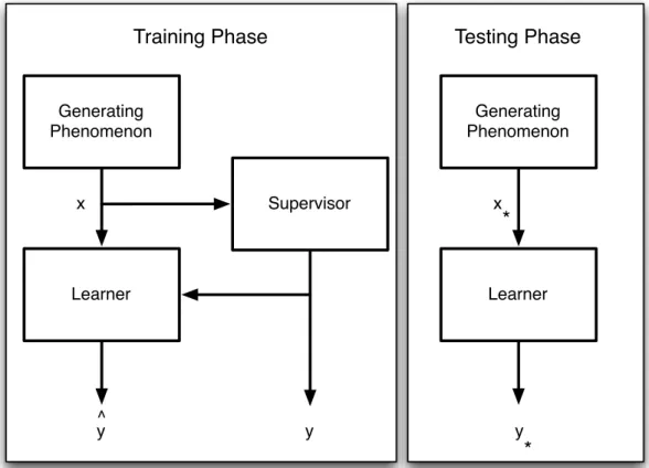
The typical supervised learning experimental setting (Bishop 2006) consists of having a training set {xi, yi}Ni=1 of N predictor and response variables that are used to learn the parameters of the assumed model (model fitting). Assuming that the input predictors are i.i.d generated from a phenomenon and the depen-dent responses from a supervisory process, the goal of learning, as depicted in Figure 2.1 is to approximate the supervisory process and predict responsey∗ of novel input samplex∗.
The learning process is driven by a loss function2 L(y,yˆ) between the esti-mated response ˆy and the true response y which measures the deviation of the prediction with respect to the true target (evidence). At this point, the specific loss function and learning procedure deviates to two main schools of thought inspired from different branches of statistics and mathematics.
2.2.1
Statistical Learning Theory
In the Statistical Learning Theory (SLT) paradigm (Vapnik 1998, Hastie et al. 2001), the emphasis is on (typically convex) optimisation with respect to specific loss functions and penalising (regularisation) terms. As an example, the simple linear regression case can be approached with the Mean Squared Error (MSE) Loss: 1 N N X i=1 |yi−yˆi|2 (2.6)
Generating Phenomenon Supervisor Learner x y y ^ Training Phase Generating Phenomenon Learner x y Testing Phase
*
*
Figure 2.1: The supervised learning setting.
whose minimisation with respect to the parametersw and the estimating func-tionf(x) = wTxleads, see Hastie et al. (2001) for first and second order deriva-tives, to the well known global minimum solution:
ˆ
wOLS = (X T
X)−1XTy (2.7)
The MSE loss results to the ordinary least-squares method by3 Gauss (1809) and the optimisation implicitly leads to minimising the noise error PN
i=1
2
i for
which we have made no assumptions so far.
To control over-fitting the estimating function to the target response (fitting the noise), regularisation via a penalising term is employed within the SLT frame-work4. In the linear regression case a typical regularisation is the squared-weight penalty λ2PD
d=1w
2
d which leads to the penalised least squares (PLS) solution: 3Also claimed by Adrien-Marie Legendre in 1805
4In later sections we also draw the connection between regularisation and sparsity of the resulting solution.
ˆ
wPLS = (X T
X+λI)−1XTy (2.8)
where the parameter λ controls the trade-off between the smoothness of the function and the fit to the data.
Finally, having briefly described the training or learning phase for linear regression with a linear function within the SLT framework, prediction can be made based on the inferred parameters (from ordinary or penalised least squares), the novel predictor and our estimating linear function as:
y∗ = ˆw T
x∗ (2.9)
2.2.2
Towards Bayesian Inference
In this section we revisit the linear regression setting and introduce the ba-sic concepts behind the Bayesian paradigm and the direct connections, e.g. (Tipping 2004), to the least squares solutions of the SLT framework.
So far we have made no modelling assumptions regarding the noise com-ponent which was implicitly minimised in the SLT case and could potentially lead to over-fitting without regularisation. In the Bayesian setting a probabilistic model over the noise component is placed which can be assumed to be normally distributed withσ2 variance: ∼ N(0, σ2I).
This directly leads to a distribution over the responses, whose negative log-arithm resembles a typical loss function, which is the likelihood of the linear model m: L=p(y|X, m) = N(f(X), σ2I) = N(Xw, σ2I) = N Y i=1 N(wTxi, σ2) (2.10)
This important distribution expresses how likely it is for the model to re-produce or generate theevidence y.
Maximisation of the likelihood is equivalent to minimising the negative log-arithm:
L=−logp(y|X, m) = N 2 log(2πσ 2 ) + 1 2σ2 N X i=1 {yn−w T xi}2 (2.11)
which leads to themaximum likelihood (ML) estimate for the parameterswthat is equivalent to the ordinary least squares estimate from Equation 2.7:
ˆ
wML = argmax w
(L) = ˆwOLS (2.12)
and analogously for the noise variance: ˆ
σML= argmax σ
(L) (2.13)
However now we have resulted again in a point estimate for the parameters5 and the response despite the initial placement of a distribution over the error component. Furthermore the ML estimate is prone to over-fitting (Ripley 1996), especially when the training size is small, as it is solely based on the data evi-dence.
2.2.3
Bayesian Inference
In order to retain a truly probabilistic framework we must also place distributions over the random variables before the model sees any evidence in the form of data. Such distributions are called prior distributions and express oura priori beliefs
about the phenomenon we are trying to infer (as prior beliefs on the model parameters imply prior beliefs for the phenomenon). In order to update these prior beliefs toa posteriori beliefs, having seen the evidence, we need Bayes rule which is the foundation of Bayesian inference:
Bayes Rule : P(A|B) = P(B|A)P(A)
P(B) (2.14)
where
• P(A) - The prior belief for A independent of B.
• P(B) - The prior belief for B independent of A. Also defined as the 5The variance of the estimate is available but has no contribution in the final prediction.
marginal likelihood as it is equivalent with integrating out A from the
joint likelihood which is the numerator.
• P(B|A) - The conditional probability of B givenA which corresponds6 to the likelihood of A for known B.
• P(A|B) - The posterior belief for A after observing B.
Returning back to the linear regression framework we place a zero-mean Gaussian prior distribution over the parameters or regression coefficients w:
p(w|α) = D Y j=1 α 2π 1/2 expn−α 2w 2 j o (2.15) where α is a common scale or inverse variance across dimensions and the prior distribution expresses our prior belief that the evidence are generated from a relatively smooth phenomenon and hence smaller weights are preferred a priori. Following Bayes rule and recalling the likelihood function in Equation 2.10 we can now update our beliefs for the parameterswto the posterior distribution (Tipping 2004): p(w|y,X, α, σ2) = p(y|X,w, σ 2)p(w|α) p(y|X, α, σ2) =N(µ,Σ) (2.16) where µ=XTX+σ2αI −1 XTy (2.17) Σ=σ2(XTX+σ2αI)−1 (2.18)
Hence now we have a closed form solution for the posterior over the pa-rameters due to the accommodating nature of linear regression where both the likelihood and the prior can be described with Gaussian distributions that give rise to a Gaussian posterior. This unfortunately will not always be the case and we will have to resort to either sampling techniques or deterministic approxima-tions that are described in later secapproxima-tions.
It is worth noting that the prior placed on the regression coefficients has an analogous function to the regularisation component within the SLT framework. 6WhenP(B|A) is treated as a function of B givenA it corresponds to a probability (dis-tribution/density) function but when is treated as a function ofA givenB it is a likelihood function.
It places a bias for smooth estimating functions and hence ensures the model is not over-fitting the data. We can further see the analogy between the approaches by maximising over the posterior and examining the mode of that distribution:
ˆ
wMAP =µ= ˆwPLS (2.19)
assumingλ=σ2α. Thus themaximum a posteriori (MAP) solution is equivalent to the PLS estimate and the parameter productσ2α has a similar function toλ of penalising complex functions and avoiding over-fitting.
This analogy is only present when we restrict our probabilistic model to resulting point estimates such as the ML or MAP solutions. In reality we have a posterior distribution over the regression coefficients and we can make full use of it through the Bayesian tool of marginalisation:
p(y∗|y,X, α, σ2) = Z
p(y∗|w, σ2)p(w|y,X, α, σ2) dw (2.20) where we see that our final predictive function is an average over the whole of the regression coefficients posterior. In the case where integration cannot be performed in closed form, the Monte Carlo estimate can be employed. The above marginalisation provides another Bayesian benefit, that of explicitly tak-ing into account the uncertainty for the parameters in the form of the posterior distribution (if it is concentrated or diffuse).
Finally, it is worth noting that we can place further prior distributions on the scales and the variance, propagating uncertainty into higher levels in the model and becoming “truly” Bayesian by marginalising over all model parameters. In some of these cases however we loose the benefit of having a closed form posterior distribution as the joint posterior over all parameters can become intractable. At this point, sampling or deterministic approximations become necessary for Bayesian inference and we will review such strategies later in this Chapter.
The Bayesian framework will be adopted for the remainder of this thesis on the basis of its advantages, most of which we have already seen. In a summary these are:
• Prior beliefs- Explicitly incorporate prior knowledge regarding the prob-lem under consideration via the prior distributions placed on the model parameters. Bayesian inference is within the so-called subjective7 probabil-7There is a great history and interesting controversy in statistics between “Bayesians” and
ity theory field (Good 1983) and accommodates prior knowledge and also prior non-informative “objective” beliefs with appropriate distributions.
• Probabilistic Responses - Instead of a single point response, a distri-bution over responses is offered via the Bayesian framework. Therefore a direct measure of the confidence of the model’s responses is offered which is crucial for decision making in critical applications such as health infor-matics or security.
• Marginalisation - Model parameters can be marginalised (integrated) out, effectively averaging over all their possible values. Very useful and informative quantities, as we shall see and employ later on, such as the marginal likelihood are based on marginalisation.
• Uncertainty- Posterior distributions directly express the uncertainty over model parameters which is taken directly into account via the process of marginalisation. Uncertainty can be encoded and propagated into higher levels of model hierarchy through the use of priors and hyper-priors (prior distributions over parameters from lower level prior distributions).
• Formality - Bayesian inference is firmly based on probability theory and the corresponding axioms of plausible reasoning (Jaynes 2003) providing a systematic and formal way of dealing with uncertainty.
2.3
The Kernel Trick and Kernel Regression
So far in this thesis we have concentrated on linear regression and how to per-form learning through the two mainstream approaches of SLT and Bayesian inference, highlighting the probabilistic benefits of the latter. We have seen how non-linearity between the input predictors and the responses can be achieved through basis function expansions while retaining the appealing nature and identifiability of linear models. In this section we take a step further into pos-sibly nonlinear embeddings of the original features and introduce the concept of kernel substitution, also known as the kernel trick, which has revolutionised
“Frequentists” on exactly the subjective nature of prior distributions. The interested reader is directed to (Jaynes 2003) and (Edwards 1992) for the Bayesian and Frequentist perspective respectively.
the field during the last decade (Sch¨olkopf and Smola 2002, Shawe-Taylor and Cristianini 2004).
Consider the basis function expansion of the linear regression model in Equa-tions 2.4 and 2.5 and generalise it to some possible nonlinear feature expansion
Φ∈RN×M with the ith row given byφ(x i)
T :
y=Φw+ (2.21)
The likelihood and prior follow from Equations 2.10 and 2.15 after substi-tuting the expansion Φ. Disregarding the marginal likelihood which is a con-stant term we can express the logarithm of the posterior8 as the sum of the log-likelihood and log-prior:
logp(w|y,X, α, σ2)∝ − 1 2σ2 N X i=1 {yi−w T φ(xi)}2− α 2w T w (2.22)
maximising with respect tow, setting to zero and solving for w we have:
w=− 1 ασ2 N X i=1 {yi−w T φ(xi)}φ(xi) =Φ T a (2.23)
where the vector a has elements ai = −ασ12{yi −w T
φ(xi)}. We can now re-formulate the logarithm of the posterior with respect to the parameter a and obtain: logp(w|y,X, α, σ2) =− 1 2σ2a T ΦΦTΦΦTa+ 1 σ2aΦΦ T y− 1 2σ2y T y−α 2a T ΦΦTa (2.24) and we can see that the feature expansion Φ appears only as an inner product with itself. Hence this dual representation indicates that we actually only need inner products of the feature expansion and not the actual feature expansion per se. Defining theN×N Gram matrixK=ΦΦT as a symmetric matrix of vector inner products in an inner product space and setting the derivative to zero with respect toa we obtain the dual solution:
8We could directly formulate the closed form posterior as in 2.16 but we will maximise over it to introduce the dual formulation and the kernel trick.
a= (K+ασ2I)−1y (2.25) which, recalling Equation 2.9, leads to the prediction for a novel samplex∗ as:
y∗ =w T φ(x∗) =a T Φφ(x∗) =k(x∗) T (K+ασ2I)−1y (2.26) where k(x∗) denotes a vector of N inner products between the training set expansionΦ and the test sample expansionφ(x∗).
This transformation of the problem leads to two main observations. First, that we do not need to explicitly construct a feature embeddingΦof the input samples but we only need to define a valid function that directly describes the inner product of some feature expansion. Secondly, the transformed regression parameters of the dual formulation are N dimensional now as they operate on the Gram matrix and they require an O(N3) inversion for estimation. This appears initially disadvantageous as we were operating before on a space with dimensions equal to the number of basis functions, which are typically less than the number of samples, but it offers the advantage that implicitly now we can employ a very high (infinite in some cases) dimensional embedding.
Definition 2.1: [Kernel function] (Shawe-Taylor and Cristianini 2004)
A kernel is a function k that for all xi,xj ∈X satisfies
k(xi,xj) =hφ(xi),φ(xj)i
whereφ is a mapping from X to an (inner product) feature space F
φ:x7→φ(x)∈F.
From Definition 2.1 we can see that the Gram matrixKis the corresponding
kernel matrix and now we can employ any valid kernel function to implicitly produce high dimensional embeddings. The main kernel property of interest at this stage (see (Shawe-Taylor and Cristianini 2004) for a full treatment) is that the resulting kernels are symmetricpositive semi-definite matrices.
Definition 2.2: [Positive Semi-definite Matrix]
Some typical kernel functions k(xi,xj) = hφ(xi),φ(xj)i that are employed in this thesis are summarised in Table 2.3:
Kernel Type Function Characteristics
Linear (Cosine) xTixj
Cosine follows by normalisation Polynomial xTixj + 1 n Degree n Gaussian (RBF) exp −||xi−xj|| 2 2σ2
Infinite degree polynomial
Finally, revisiting the linear regression setting we can now reformulate it into akernel regression problem:
y=wTK+ (2.27)
and as before we obtain a closed form Gaussian posterior distribution for the regression coefficients as p(w|y,K, α, σ2) = N(µ,Σ) with parameters defined with respect to the kernel matrixK as:
µ=KTK+σ2αI
−1
KTy (2.28)
Σ=σ2(KTK+σ2αI)−1 (2.29)
The kernel trick offers a powerful and efficient way of producing high di-mensional data embeddings that capture non-linearities of the modelling phe-nomenon and will be of especial interest to the classification setting that we visit next.
2.4
Classification
In classification the target or response variables9 tare discrete real values asso-ciating input samplesxi to a single specific class c∈ {1, . . . , C}. The encoding for the target varies depending on the classification model employed and the number of classes. For binary classification problems where there are only two classes it is typically represented as tn ∈ {0,1} or tn ∈ {−1,+1} whereas for multinomial problems it is eithertn ∈ {1, . . . , C}or follows a 1−of−C encoding scheme.
The interest lies in the joint distribution p(t,X) and there are two main categories of classification models depending on its decomposition:
p(t,X) =p(t|X)p(X) =p(X|t)p(t) (2.30) Following the first decomposition, we end up directly modelling the quantity of interestp(t|X) and such models are termeddiscriminative. In the second case we model the class conditional densityp(X|t) and employ Bayes’ rule to obtain again the distribution of interest:
p(t|X) = p(X|t)p(t)
p(X) (2.31)
Such approaches are termed generative as we are able to generate samples from the model’s class conditional distribution. There are qualitative differences and merits for either approach (Duda et al. 2000, Bishop 2006) and in this thesis we concentrate ondiscriminative approaches which avoid the drawbacks of density estimation in high-dimensional spaces and directly model the quantity of interest p(t|X).
2.4.1
Logistic and Probit Regression
The standard probabilistic discriminative classification approach is to turn the output of a regression model into a class probability by the use of a sigmoid
function10. This constrains the continuous real value output [−∞,+∞] to the range [0,1], satisfying the requirements for a probabilistic representation of class membership.
For example, in the linear regression case the model becomes:
t=σwTh(x) (2.32)
where the sigmoid function σ typically takes one of the following forms:
Type Function Case Logistic σ(z) = exp(z) 1 + exp(z) Binary Softmax σ(zc) = exp(zc) PC i=1exp(zi) Multinomial Probit Φ(z) = Z z −∞ Nx(0,1)dx Binary
These approaches belong to the family of Generalised Linear Models (GLMs) (McCullagh and Nelder 1989) and are specifically known as logistic or probit
regression, according to the likelihood function employed11.
Considering now the general probabilistic classification framework with GLMs we have the posterior for the parameters w:
p(w|t,X, α) = R p(t|X,w)p(w|α)
p(t|X,w)p(w|α)dw (2.33)
where the likelihoodp(t|X,w) is given by the specific choice of link function in Table 2.4.1.
Unfortunately the posterior cannot be obtained in closed form, in contrast with the accommodating nature of linear regression models, and hence exact
inference is not possible. This is a typical obstacle in Bayesian inference for which approximate methods have been proposed and developed. In the next sections we review exactly such approximate inference techniques that will allow us to complete inference within the classification setting.
2.5
Markov Chain Monte Carlo
The first approximate inference scheme reviewed is the sampling approaches of Markov chain Monte Carlo (MCMC) which becomes exact in the limit of infinite samples. For an excellent practical introduction the reader is referred to Gelman et al. (2004). The intuition behind MCMC is to address our inability of obtaining closed form posterior distributions by instead drawing samples from them.
In most cases we are actually interested in calculating expectations with re-spect to the posterior distribution, such as the class predictions in classification.
Hence, assuming we can draw samples from the (joint) posterior of parameters12 θ, these expectations can be approximated via the Monte Carlo estimate:
E{f|t,X}= Z f(θ)p(θ|t,X)dθ ≈fe= 1 L L X l=1 f(θl) (2.34)
One important observation is that the variance of the Monte Carlo estimate is given by: var{fe}= 1 LE (f −E{f})2 (2.35)
and hence the accuracy of the estimate is independent of the model’s dimension-ality.
The major hurdle of sampling from the posterior distribution has not been addressed so far and in the next section the four sampling approaches that will be employed in this thesis are reviewed.
2.5.1
Importance Sampling
One of the most classical, and straightforward to implement, Monte Carlo esti-mators for a functionf(θ) withθ distributed asp(θ) is given by the importance sampling approach that utilises an easy-to-sample from distributionq(θ) in the following way: Ep(θ){f(θ)}= Z f(θ)p(θ)dθ= Z f(θ)p(θ) q(θ)q(θ)dθ =Eq(θ){w(θ)f(θ)} (2.36) wherew(θ) = p(θ)
q(θ) is the importance weight.
The intuition behind this approach is to sample from theimportance distri-butionq(θ) which can be conveniently chosen as long as it offers good support for the distribution of interest, and then to weight each sample with the associated importance weight resulting in the following estimator:
12In order to express any model parameter and not only regression coefficientsw, we denote parameters with the generic notationθ. We assume the classification setting as an example scenario with the parameter posterior of interestp(θ|t,X).
e f = 1 L L X l=1 w(θl)f(θl) (2.37)
In the (common) case (Andrieu 2003) where the distribution of interestp(θ) is only available in its unnormalized formp∗(θ) then the importance weights are modified to: w(θl) = p∗ θl q(θl) N X j=1 p∗(θj) q(θj) (2.38)
Finally, the main dangers of importance sampling reside in the choice of the importance distribution. Ideally it should offer support so that the tar-get distribution is efficiently explored and it should satisfy the condition that
p(θ) > 0 ⇒ q(θ) > 0. The advantages of importance sampling are that it’s easy to implement, it is parallelisable, and that it can be extended to sequential inference. Due to the latter property it is the cornerstone of sequential Monte Carlo (particle filters) techniques (Doucet et al. 2000) and the main approach in dealing with covariate shift (Qui˜nonero-Candela et al. 2009) where the i.i.d assumption is no longer valid.
In the next sections we introduce the Markov chain Monte Carlo techniques that construct anergodic Markov chain that converges to astationary distribu-tion that is the target distribudistribu-tion. The following definidistribu-tions introduce the basic concepts:
Definition 2.3: [First order Markov chain]
A first order Markov chain is a sequence of random variables θ1, θ2, ..., θn that for
any t ∈ {1, . . . , n} the distribution of θt given all previous values of θ is dependent
only on the previous valueθt−1:
p(θt|θt−1, θt−2, . . . , θ1) =p(θt|θt−1)
Definition 2.4: [Ergodicity]
A Markov chain converges to a unique stationary distribution if it is irreducible, aperiodic and not transient. Such a Markov chain is called ergodic.
Where aperiodicity and non-transiency hold for a random walk on any proper distribution (Gelman et al. 2004) and irreducibility dictates that there is a pos-itive probability of reaching any state from any other state, in other words the Markov chain can reach all states from any state within a finite sequence of steps.
2.5.2
Metropolis Sampling
The first MCMC method considered is the Metropolis algorithm (Metropolis et al. 1953) which employs a symmetric proposal distribution (also known as transition or jump distribution) q(θt|θt−1) = q(θt−1|θt) and accepts or rejects generated samples from that distribution based on the following criterion known as theacceptance ratio:
R= min 1, p∗(θ t|t,X) p∗(θt−1|t,X) (2.39) where p∗(θ|t,X) denotes the unnormalized parameter posterior which is equal to the product of the likelihood with the prior over the parameters.
The procedure is to draw a random number from a uniform distribution on the unit interval and if the number is smaller or equal tomathcalRthe proposed sample is accepted, else rejected. Hence the new state is given by:
θt= (
θt with probabilityR
θt−1 otherwise (2.40)
2.5.3
Metropolis-Hastings Sampling
The straightforward generalisation of the Metropolis scheme to handle asymmet-ric proposal distributions is known as the Metropolis-Hastings (MH) method. The only significant difference is that the distributionq(θ) is asymmetric: q(θt|θt−1)6=
q(θt−1|θt) and hence it is included in the acceptance ratio as:
R = min 1, p∗(θ t|t,X)q(θt−1|θt) p∗(θt−1|t,X)q(θt|θt−1) (2.41) Both the Metropolis and the Metropolis-Hastings MCMC methods have been proved (Hastings 1970) to converge to a stationary distribution that is the target distribution (p(θ|t,X) here).
The main drawback of Metropolis based MCMC methods is the need to
tune the proposal distribution in order to retain an acceptance ratio between 15−40% (depending on the nature of the parameter sampling scheme) which is the recommended level to efficiently reach convergence (Gelman et al. 2004). Adaptive proposal distributions are usually employed that take into account the covariance structure of the posterior through initial exploratory samples that are later discarded (Burn-in period). In general, the engineering requirements of such methods make them less practical although more efficient sampling schemes based on gradient information through the Fisher information matrix are a major research topic (Girolami et al. 2009) and a promising direction.
2.5.4
Gibbs Sampling
The final MCMC approach reviewed is the Gibbs sampler (Geman and Geman 1984, Tanner and Wong 1987) also known as alternating conditional sampling
(Andrieu 2003, Gelman et al. 2004) which can be seen as a special case of the Metropolis-Hastings method. The intuition behind it is to decompose the (un-obtainable in closed form) posterior distribution of interest into conditional pos-terior distributions that are easy to sample from. Consider a parameter vectorθ and the sought after posterior distributionp(θ|t,X). If we decompose the joint posterior to conditional posterior distributions of the form:
p(θti|θt−−1i ,t,X) (2.42)
then iteratively sampling from these conditional distributions leads to sampling from the target joint posterior distribution. The notation θt−−1i denotes all the elements ofθ except the ith one, from the current (t−1) sample.
This principle can be extended to sampling block variables where the joint posterior can be decomposed to blocks of parameter sets (i.e. regression co-efficients w and scales α in GLMs) whose conditional posterior distributions are easy to sample from. Such a block-wise Gibbs sampling approach will be employed in this thesis.
The advantage of Gibbs sampling is that no proposal distribution is necessary. It can be seen as a sub-case of MH sampling with an acceptance ratio equal to one, see e.g. Gelman et al. (2004) for proof, and this alleviates the need for tuning acceptance ratios and adapting proposal distributions for efficient exploration of