A University of Sussex MPhil thesis
Available online via Sussex Research Online:
http://sro.sussex.ac.uk/
This thesis is protected by copyright which belongs to the author.
This thesis cannot be reproduced or quoted extensively from without first
obtaining permission in writing from the Author
The content must not be changed in any way or sold commercially in any
format or medium without the formal permission of the Author
When referring to this work, full bibliographic details including the aut
hor, title, awarding institution and date of the thesis must be given
models
Pietro Galliani
University of Sussex
I hereby declare that this thesis has not been and will not be submitted in whole or in part to another University for the award of any other degree.
The bulk of this thesis is taken from a paper with the same title, fruit of a collaboration between myself (first author), Edwin Bonilla, Amir Dezfouli and Novi Quadrianto, which has been accepted at AISTATS 2017 conference and has been published in its proceedings.
Contents
1 Introduction 4
1.1 Structured prediction . . . 4
1.2 Related work . . . 6
1.3 This work . . . 10
2 Gaussian Process Models for Structured Prediction 11 2.1 Conditional Random Fields and Gaussian Processes . . . 11
2.2 Linear chain structures . . . 13
3 Automated Inference 16 3.1 Generalising the Nugyen-Bonilla class of models . . . 16
3.2 Automated variational inference . . . 17
4 Sparse Approximation 20 4.1 Evidence lower bound . . . 21
4.2 Expectation estimates . . . 22
5 Learning 23 5.1 Computational complexity . . . 23
5.2 Variance reduction . . . 24
5.3 Piecewise pseudo-likelihood . . . 25
5.4 Making and evaluating predictions . . . 26
6 Experiments 26 6.1 Datasets and experimental baselines . . . 26
6.2 Small-scale experiments . . . 27 6.3 Larger-scale experiments . . . 29 6.4 Discussion . . . 29 7 Conclusion 30 7.1 Future Work . . . 30 7.2 Concluding Remarks . . . 30 8 Bibliography 32 Appendices 34
A Proof of Theorem 2 34
A.1 Estimation ofLell in the full (non-sparse) model . . . 35
A.2 Gradients . . . 35
B KL terms in the sparse model 36 C Proof of Theorem 3 37 D Gradients ofLelbo for sparse model 38 D.1 Inducing variables . . . 38
D.1.1 KL term . . . 38
D.1.2 Expected log likelihood term . . . 39
D.1.3 Pairwise functions . . . 40
E Experiments 40 E.1 Experimental set-up . . . 40
E.2 Optimization . . . 42
E.3 Performance profiles . . . 42
Abstract
We develop an automated variational inference method for Bayesian structured prediction problems with Gaussian process (gp) priors and linear-chain likelihoods. Our approach does not need to know the details of the structured likelihood model and can scale up to a large number of observations. Furthermore, we show that the required expected likelihood term and its gradients in the variational objective (ELBO) can be estimated efficiently by using expectations over very low-dimensional Gaussian distributions. Optimization of the ELBO is fully parallelizable over sequences and amenable to stochastic optimization, which we use along with control variate techniques to make our framework useful in practice. Results on a set of natural language processing tasks show that our method can be as good as (and sometimes better than, in particular with respect to expected log-likelihood) hard-coded approaches including svm-struct andcrfs, and overcomes the scalability limitations of
previous inference algorithms based on sampling. Overall, this is a fundamental step to developing automated inference methods for Bayesian structured prediction.
1
Introduction
1.1
Structured prediction
Structured prediction problems are prediction problems in which the available data is best understood as consisting of structured objects (that is, objects with a non-trivial internal
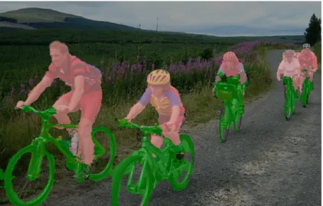
Figure 1: An example of image segmentation: pixels of the imagine are labeled as belonging to bikes (green overlay), people (red overlay), or neither (no overlay). Segmentation based on the CRF-as-RNN algorithm of (Zheng et al., 2015). Image taken fromhttp://www.robots.ox.ac. uk/~szheng/crfasrnndemo.
relational structure), rather than as consisting of scalar values or as values in some fixed-dimensionality vector (Bakir, 2007). Alternatively, structured prediction problems may be seen as problems in which there exist relationsbetween different elements of the dataset.
The duality between these two views can be seen easily in two typical instances of structured prediction problems, namelyimage segmentation (Luccheseyz and Mitray, 2001) and Part-of-Speech tagging (Voutilainen, 2003).
The problem of image segmentation, in brief, consists in partitioning the pixels of a digital image in sets belonging to different categories (e.g. to the foreground/to the background, or to different physical objects), as shown for instance in Figure 1. Under the first view, each component of our data is an entire image, with the features ascribed to each pixel as well as a specification of the relative positions of these pixels; and the result of the prediction consists itself of a complex object which fixes a label for each pixel of the image.
The second view, on the other hand, allows us to regard each individual pixel as a distinct element of our data. This lets us ignore the problem of producing a complex output, as every pixel must be matched to one single label; but the cost of this is that under this view there exist relationsbetween components of our data – i.e., spatial relationships between pixels of the same image – which carry information which is relevant to the prediction task. In particular, under this view it is not possible to assume, as it is often done in prediction tasks, that observations and labels are independently and identically distributed: the features and the labeling of a pixel, indeed, are not by any means independent from those of its neighbours.
Figure 2: A simple example of Part-of-Speech tagging: in the sentence “Nobody leaves the room”, the word “leaves” is identified as a verb (rather than a noun or some other category). It would be impossible to make such a prediction on the basis of the features of the word “leaves” alone: in order to identify the category to which a word belongs, it is also necessary to consider its position with respect to the other words of its sentence.
natural language sentence, the category to which each word belongs. Again, there are two equivalent ways of understanding this problem: we can say that whole sentences (or even entire paragraphs or texts) are distinct elements of our data, and require that the outputs of our algorithm to be same-length sequences of word labelings, or we can say that the elements of our data are single words and the required outputs are the corresponding labelings. This view, again, allows us to eschew the difficulty of our algorithm returning complex structures as output, but at the cost – once more – of having relationsbetween objects of our data (e.g. neighbourhood relations between words) which are relevant to their correct labeling, as well as at the cost of losing the assumption that the elements of our datasets are identically and independently distributed (i.i.d).
1.2
Related work
As already mentioned, structured prediction refers to the problem where there are interdepen-dencies between samples and it is necessary to model these depeninterdepen-dencies explicitly. Common examples are found in natural language processing (nlp) tasks, computer vision and bioinfor-matics. By definition, observation models in these problems are not i.i.d and standard learning frameworks have been extended to consider the constraints imposed by structured prediction tasks. Popular structured prediction frameworks are conditional random fields (crfs; Lafferty et al., 2001), maximum margin Markov networks (Taskar et al., 2004) and structured support vector machines (svm-struct, Tsochantaridis et al., 2005):
• Conditional random fields will be discussed in some detail in Section 2.1. In brief, they are discriminative, undirected probabilistic graphical models in which the weights associated tofactors between variables are (generally linear) functions of the features of the individual variables (e.g. pixels or words) involved. The probability distribution over the (structured) outputs is then derived from those weights by means of the softmax function, as shown in Equation (2).
• Maximum margin Markov networks make use of margin-based optimization to learn the parameters of (generative) probabilistic graphical models, namely Markov networks. The
optimization algorithm makes use of thekernel trick (Aizerman, 1964) in order to operate over high-dimensional feature spaces without representing them esplicitly, and seeks the choice of parameter which maximizes the separation between classes. This problem is then reparametrized in a way that allows for an efficient solution, as long as the loss function can be decomposed in the same way as the feature map.
• Similarly to maximum margin Markov networks, thesvm-struct framework also extends to the structured classification case the maximum margin approach of support vector machines (svm); but, differently from the cases of conditional random fields and maximum margin Markov networks, it is not a type of probabilistic graphical model and it does not return a probability distribution over the possible labelings, but just predictions for the correct labelings. svm-struct makes use of a cutting plane algorithm in to solve certain quadratic optimization problems with exponentially many constraints in polynomial time.
Recurrent neural networks have also been used for certain structured prediction tasks (see e.g. Graves et al., 2012). Here we mention a novel and exciting approach is the exploration of the connection between conditional random fields and recurrent neural networks (Zheng et al., 2015), which allows for the possibility of treating conditional random fields as layers of a neural network architecture. The chief insight of (Zheng et al., 2015) is that one of the inference methods for conditional random fields, namely mean-field inference (Krähenbühl and Koltun, 2011), can be reformulated within the formalism of recurrent neural networks and then added as a layer to more complex neural networks. This approach promises to combine the advantages of neural networks and probabilistic graphical models for structured prediction.
Gaussian Processes (gp) are probability distributions over functions that may be thought of as infinite-dimensional generalisations of multivariate normal distributions. Formally, they may be defined (Rasmussen and Williams, 2006), as a collection of random variables, any finite number of which have a joint Gaussian distribution specified by a mean (often assumed to be constantly zero) and a covariance defined in terms of akernel functionκ(x,x0). Their application to (non-structured) regression and classification is largely due to the fact that conditioning multivariate normal distributions with respect to observed values yields another multivariate normal distribution having a straightforward and elegant form: if
f(x) f(x0) ∼ N 0, κ(x,x) κ(x,x0) κ(x0,x) κ(x0,x0)
then the probability distribution off(x0)conditioned over an observed value off(x)is given by
f(x0)|f(x)∼ N(κ(x0,x)κ(x,x)−1f(x), κ(x0,x0)−κ(x0,x)κ(x,x)−1κ(x,x0)). (1) A similar, only slightly more complicated expression applies in the case that the observations
f(x)are subject to (additive and i.i.d.) Gaussian noise ∼ N(0, σ2).
Gaussian Processes can be used as the key component of powerful and elegant nonparametric probabilistic machine learning models. However, their asymptotic computational performance often does not compare favourably to that of other approaches to regression or classification, due largely to the fact that computing (1) requires inverting the matrixκ(x,x), which is of size
N×N whereN =|x|is the number of observed samples. As inverting such a matrix carries
O(N3)time complexity if this is done via Gaussian elimination1, such an approach to regression or classification is not feasible even for comparatively small datasets.
Two techniques, however, have been recently used with good success to improve the compu-tational performance of Gaussian Process-based regression and classification models:
• Sparse Gaussian Processes (Snelson and Ghahramani, 2006) differ from Gaussian Processes in that the conditioning of Equation (1) is not performed directly with respect to the training data(x,f(x))but rather with respect to a smaller set ofM N pseudoinputs z, whose locations and corresponding valuesf(z)can be chosen in a way that attempts to maximize the likelihood of the training data(x,f(x)). The cost of the matrix inversion is thenO(M3), which for suitable choices ofM may lead to a computationally feasible model which anyway has good performance.
• Variational approximation techniques approximate thegpposterior (1) with a function
g of known form. The task is then to learn the parameters ofg in order to minimize a distance (espressed in terms of Kullback-Leiber divergence) between g and the true posterior.
Recent advances in sparsegpmodels for regression (Titsias, 2009; Hensman et al., 2013), which combine the two approaches mentioned above by drawinggfrom Gaussian Processes conditioned over the pseudoinputsz(whose positions and values are then the parameters with respect to which the KL divergence is minimized) have allowed the applicability of such models to very large datasets, opening opportunities for the extension of these ideas to classification and to non-structured problems with generic likelihoods (Hensman et al., 2015a; Nguyen and Bonilla,
1This is not asymptotically optimal – for instance, the Coppersmith–Winograd algorithm for matrix inversion
(Coppersmith and Winograd, 1987) carries a time complexity of∼O(N2.376)– but it is often done in practice
anyway due to numerical stability concerns and to the constant factors hidden by the asymptotic notation (Robinson, 2005).
2014; Dezfouli and Bonilla, 2015; Hensman et al., 2015b). However, none of these approaches is actually applicable to structured prediction problems, which inherently deal with likelihoods that do not factorize over individual samples.
A related, exciting area of research in machine learning which plays a major role in the above described research direction consists in the development of automated inference methods for complex probabilistic models, with notable examples in the probabilistic programming community given bystan(Hoffman and Gelman, 2014) andchurch(Goodman et al., 2008). The principal thrust of this enterprise consists in the development of models and algorithms that may be deployed over a wide range of models and cost functions with a minimal amount of human intervention and fine-tuning. One of the main challenges for these approaches is to formulate expressive probabilistic models and develop generic yet efficient inference methods for them. From a variational inference perspective, one particular approach that has addressed such a challenge is the black-box variational inference framework of Ranganath et al. (2014). In brief, Ranganath et al. (2014) presents a variational optimization method for probabilistic models with latent variables in which the divergence between the variational approximation and the true posterior is minimized via a stochastic optimization algorithm, and the needed gradients are estimated via sampling. Crucially, the algorithm is largely agnostic with respect to the choice of model and likelihood, allowing the user to try out a vast range of models and likelihoods without need for time-consuming derivations.
While the works of Hoffman and Gelman (2014) and Ranganath et al. (2014) have been successful with a wide range of priors and likelihoods, their direct application to models with Gaussian process (gp) priors is cumbersome, mainly due to the large number of highly coupled latent variables in such models. In this regard, very recent work has investigated automated inference methods for general likelihood models when the prior is given by a sparse Gaussian process (Hensman et al., 2015b; Dezfouli and Bonilla, 2015). The framework of (Dezfouli and Bonilla, 2015), in particular, is at the basis of the one discussed in this work, and can be seen as the limit case (for sequences of length one) of the variational approximation approach described in detail in §3 and §4. However, while these advances have opened up opportunities for applying gp-based models well beyond regression and classification settings, they have focused on models with i.i.d observations and, therefore, are unsuitable for addressing the more challenging task of
structured prediction.
From a non-parametric Bayesian modeling perspective, in general, and from agpmodeling perspective, in particular, structured prediction problems present very hard inference challenges because of the rapid explosion of the number of latent variables with the size of the problem. Furthermore, structured likelihood functions are usually very expensive to compute.
Twin Gaussian processes (Bo and Sminchisescu, 2010) address structured continuous-output problems by forcing input kernels to be similar to output kernels. In contrast, here we deal with the harder problem of structureddiscrete-output problems, where one usually requires computing expensive likelihoods during training. The structured continuous-output problem is somewhat related to the area of multi-output regression withgps for which, unlike discrete structured prediction withgps, the literature is relatively mature (Álvarez et al., 2010; Álvarez and Lawrence, 2011, 2009; Bonilla et al., 2008).
In an attempt to build non-parametric Bayesian approaches to (non-continuous) structured prediction, Bratières et al. (2015) have proposedgpstruct, a framework based on acrf-type modeling approach withgps which uses elliptical slice sampling (ess; Murray et al., 2010) as part of its inference method. Unfortunately, although their method can be applied to linear chain structures in a generic way without considering the details of the likelihood model, it is not scalable as it involves sampling from the fullgpprior. We refer to §2.1 and §2.2 for a more detailed discussion (sans elliptical slice sampling) of the approach of Bratières et al. (2015), on which the approach discussed in this work is directly based.
Bratières et al. (2014) have explored a distributed version ofgpstructbased on the pseudo-likelihood approximation (Besag, 1975) where several weak learners are trained on subsets of gpstruct’s latent variables and bootstrap data, testing the resulting model with respect to image segmentation tasks. However, within each weak learner, inference is still done viamcmc. A variational alternative forgpstruct inference (Srijith et al., 2014, 2016) is also available. However, it relies on pseudo-likelihood approximations, which in the (non-sparse) approach discussed in the paper are essential for the tractability of the algorithm, and was only evaluated on small-scale problems.
1.3
This work
In this work we present an approach for automated inference in structuredgpmodels with linear chain likelihoods that builds upon the structuredgpmodel of Bratières et al. (2015) and the sparse variational framework of Dezfouli and Bonilla (2015) (which, in turn, is a sparse variant of the variational framework of Nguyen and Bonilla (2014)). In particular, we show that the model of Bratières et al. (2015) can be mapped onto a generalization of the automated inference framework of Dezfouli and Bonilla (2015). Unlike the work of Bratières et al. (2015) our approach is scalable to a large number of observations, as it makes use of sparsegp priors; and unlike the work of (Srijith et al., 2014, 2016), our approach can deal with both pseudo-likelihoods and generic (linear-chain) structured likelihoods, and we rely on our sparse approximation procedure and our automated variational inference technique – rather than on bootstrap aggregation – to
achieve good performance on larger datasets.
More importantly, this approach is also generic in that it does not need to know the details of the likelihood model in order to carry out posterior inference. Finally, we show that our inference method is computationally efficient in that it only requires expectations over low-dimensional Gaussian distributions in order to carry out posterior approximation.
Our experiments on a set of nlp tasks, including noun phrase identification, chunking, segmentation, and named entity recognition, show that our method can be as good as (and sometimes better than, in particular with respect to expected log-likelihood) hard-coded ap-proaches includingsvm-struct andcrfs, and overcomes the scalability limitations of previous inference algorithms based on sampling.
We refer to our approach as “gray-box” inference since, in principle, changing the structure of the underlying graphical model (for instance, moving from a linear chain model to a skip-chain model, or extending a grid model for image processing by introducing factors between non-neighbouring pixels) cannot be done automatically. Nevertheless, when applied to fixed structures, our proposed inference method is entirely “black box”. For example, as we will see, we can replace the exact likelihood with a pseudo-likelihood without needing to make any other modifications to our code.
2
Gaussian Process Models for Structured Prediction
2.1
Conditional Random Fields and Gaussian Processes
We are interested in structured prediction problems in which we observe input-output pairs
D={Xn,yn} Nseq
n=1, where
• Nseq is the total number of observations;
• Xn∈ X is a descriptor of observationn;
• yn∈ Y is the output corresponding to observationn;
• Xn and/or yn are structured objects such as a sequence, a tree or a grid, that reflect the
interdependences between its individual constituents.
Given a new input descriptorX?, our goal is to predict its corresponding structured labely?
and, more generally, a distribution over these labels.
Conditional Random Fields crf (Lafferty et al., 2001; Sutton et al., 2012) are discrimi-native undirected probabilistic graphical models which constitute a state-of-the-art approach to structured prediction. In CRFs, relationships between variables (e.g. between the labels
of neighbouring pixels or words, or between the labels of pixels/words and the corresponding features) are represented asfactors whose values are (generally linear) functions of the features of the variables involved.
Beingdiscriminative probabilistic models, CRFs specify the conditional distributionp(y|X)
of the labelsy given the inputsX. Generative probabilistic models for structural learning such as, for instance, Hidden Markov Models (Rabiner and Juang, 1986) would instead specify the joint distributionp(X,y).
Since CRFs are also undirected, their factors cannot in general be understood as conditional distributions specifying the probabilities of the values of a variable given those of the other variables. Instead, the probability distribution of a conditional random field can be expressed in terms of the values that factors take overcliques of variables pairwise connected by factors. More precisely, we can write
p(y|X,f) = exp ( P cf(c,Xc,yc)) P y0∈Yexp ( P cf(c,Xc,y0c)) , (2) where
• Xc andyc are tuples of nodes belonging to cliquec;
• Everyf(c,Xc,yc)is a (linear) function of the values of the features of the nodes in the
cliquec;
• The learning algorithm must seek good choices of weights for these linear combinations.
Calculating directly the value of Equation 2 is rarely computationally feasible. The difficulty, in brief, is in computing the expression at the denominator, which involves a sum over all possible labelings of the structure (whose number of increases exponentially with the size of the structure).
Various techniques, such as for instance sampling-based approaches or loopy belief propaga-tion, are used to approximate efficiently the value of the above expression. When the graph associated to the structure does not contain cycles, however, there existmessage propagation algorithms which can be used to efficiently and exactly compute the value of (2). Among the simplest of these algorithms is theforward-backward algorithm, which is applicable tolinear chain structures (discussed in the next section) and whose complexity is only linear with respect to chain length and quadratic with respect to the number of (individual) labels. We refer to Guo and Hsu (2002) for a more in-depth discussion of inference in probabilistic graphical models.
In Bratières et al. (2015), a generalization ofcrf-type models was proposed in which the
with a given covariance functionκ(·,·;θ), withθ being the hyperparameters. It is clear that such a model is a generalization of vanillacrfs where the potentials are draws from agpinstead of being (linear) functions of the features; and, as shown in Bratières et al. (2015), this approach leads to performances which are comparable or superior to those of conditional random fields and structured support vector machines (Tsochantaridis et al., 2005), another class commonly used structured prediction models. However, the use ofgppriors leads to computational costs that severely hamper the scalability of this type approach: indeed, the time complexity of this approach grows asO(N3), whereN is the number ofindividual samples (e.g. individual words
or pixels) in the dataset.2
The present work is an attempt to improve the scalability of (Bratières et al., 2015) by means of two main techniques:
1. Probabilities are computed not via sampling from the (computationally expensive) posterior distribution, but rather through avariational approximationwhich generalizes to structured model the variational approach to Gaussian Processes of (Nguyen and Bonilla, 2014);
2. The Gaussian Process itself is replaced with asparsegpapproximation after the way of (Quiñonero-Candela and Rasmussen, 2005) and (Titsias, 2009).
These two techniques were already combined in (Dezfouli and Bonilla, 2015), yielding an efficient sparse variational framework for (non-structured) Gaussian process models with black-box3 likelihoods. The present work, thus, is an attempt to use the insights of (Dezfouli and
Bonilla, 2015) to derive a more scalable version of thegp-based approach to structured prediction of (Bratières et al., 2015).
2.2
Linear chain structures
In this work we focus on linear chain structures where the output corresponding to datapointn
is a linear chain of lengthTn, whose corresponding constituents stem from a common set.
In other words, there are two types of cliques in linear chain structures, both of which involve only two nodes:
1. Unary cliques, which describe the relationship between the featuresxtat a given point of
the chain and the corresponding labelyt;
2. Binary cliques, which describe the relationship between a labelytof a non-terminal node
of a chain and the labeltn+1of its successor.
2In brief, this is due to the necessity of inverting theN×Ncovariance matrices of the Gaussian Processes. 3In the sense that different choices of likelihood could be used without deriving new expressions for the
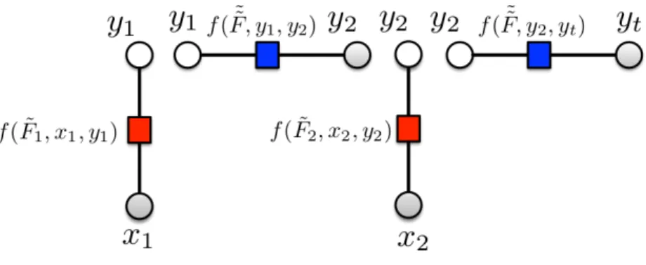
Figure 3: A linear chain model. Unary cliques are in red, binary cliques are in blue. The values
f( ˜Fi, xi, yi)are the factors corresponding to unary cliques for Equation (2), while the values
f(F˜˜i, yi, yi+1)are the factors for the binary cliques.
Linear chain structures are well-suited for applications, for instance, in natural language processing; and they have the significant advantage that the corresponding softmax likelihoods, as defined in Equation (2), can be computed in an efficient way via the forward-backward algorithm, whose complexity is of the order of|V|2T whereT is the length of the sequence and
|V|is the number of labels. This is a significant improvement over a brute-force application of Equation (2), which would require us to sum over all|V|T possible state assignments for a total
complexity ofO(T|V|T). Figure 3 shows a typical instance of linear chain structure, together
with the factors f( ˜Fi, xi, yi)andf(F˜˜i, yi, yi+1)corresponding to unary and binary factors in
Equation (2).
In this setting, the input Xn for observation n is a Tn×D matrix
x1 . . . xTn of feature
descriptors andyn is a the corresponding output sequence(y1. . . yTn)ofTn labels drawn from
the same vocabularyV.
In order to completely define the prior over the clique-dependent latent functions in Equation (2), it is now necessary to specify covariance functions over the cliques. To this end, Bratières et al. (2015) propose a kernel that is non-zero only when two cliques are of the same type, i.e. both are unary cliques(t,xt, yt)or both are pairwise cliques (yt, yt+1). These kernels are
defined as
κun((t,xt, yt),(t0,x0t0, yt0)) =I[yt=yt0]κ(xt,x0t0),
κbin((yt, yt+1),(yt0, yt0+1)) =I[yt=yt0∧yt+1=yt0+1],
whereκun is the covariance on unary functions and κbin is the covariance on pairwise functions.
In other words, according to the prior distribution of (Bratières et al., 2015)
X0 are similar (that is, if κ(xt,x0t0) is high) then, for all possible labels y, the factors
f( ˜Ft,xt, y)andf( ˜Ft0,x0t0, y)that correspond to the assignment of the labely for the two
positions (and which affect the likelihood of the labeling as per Equation 2) are also close. The relative positionstandt0 of the nodes in the corresponding chains are not relevant to this, and the distribution of these weights is independent from the distributions of the
f( ˜Ft00,xt00, y00)for other labelsy006=y.
• The probability distribution of the weightsf(F, y˜˜ t, yt+1)to be assigned to a pair(yt, yt+1)
of labels appearing at positions(t, t+ 1)is uniform and independent from the distributions of factors to unary cliques or to other binary cliques (corresponding to other positions or to other choices of labels).
This choice ofgpkernel describes – with a suitable ordering of the latent functions – a distribution with a block-diagonal covariance matrix. Its first|V|blocks, each of which describes (for the corresponding labely) the covariances between the values of the unary factorsf( ˜Ft,xt, y), are
of size P
nTn each. The last block, corresponding to covariances between pairwise factors
f(F, y˜˜ t, yt+1), is a diagonal (identity) matrix of size|V|2, where|V|denotes the vocabulary size.
To carry out inference in this model, Bratières et al. (2015) propose a sampling scheme based on elliptical slice sampling (ess; Murray et al., 2010). In the following section, we show an equivalent formulation of this model that leverages the general class of (non-structured) models presented by Nguyen and Bonilla (2014). Understanding structuredgpmodels from such a perspective will allow us to generalize the results of Nguyen and Bonilla (2014); Dezfouli and Bonilla (2015) in order to develop an automated variational inference framework. The advantages of such a framework are that of (i) dealing with generic likelihood models; and (ii) enabling stochastic optimization techniques for scalability to large datasets.
Different choices of prior are of course possible: for instance, it might be useful to deal separately with the distributions of the prior weights to the first or last nodes of the chains. However, in what follows we will using essentially the same prior described above and used in Bratières et al. (2015).4 This will allow us to make a more straightforward evaluation of
the effect of the variational approximation (based on the work of Nguyen and Bonilla (2014); Dezfouli and Bonilla (2015)) on the performance of the resulting system.
4The main differences are that the kernel functions corresponding to different labels will not necessarily be
the same and that the pairwise component of the covariance matrix will not be necessarily required to be the identity.
3
Automated Inference
3.1
Generalising the Nugyen-Bonilla class of models
Nguyen and Bonilla (2014), building upon the work of Opper and Archambeau (2009), developed an automated variational inference framework for a family of class models with Gaussian process priors. Although such an approach is an important step towards black-box inference withgp priors, since it assumes i.i.d observations it is, by definition, unsuitable for structured models.
One way to generalize such an approach to structured models such as the ones described in §2.2 is to differentiate betweengp priors over latent functions on unary nodes andgp priors over latent functions over pairwise nodes. More importantly, rather than considering likelihoods that factorize over the individual samples of our dataset, we assume likelihoods that factorize over sequences while allowing for statistical dependences within a sequence.
As in the case of the choice of kernel used in (Bratières et al., 2015) and discussed in the previous section, the prior probability distributions of the factors of unary cliques corresponding to different labels will be made to be independent, as will the prior probability distributions of different binary cliques. Furthermore, all prior distributions over the factors for unary cliques will be independent from the prior distributions over the factors for binary cliques.
Therefore, our prior modelp(f) =p(fun)p(fbin)for linear chain structures will decompose as
p(f) = |V| Y j=1 N(fjun;0,Kj) N(f bin;0,Kbin), (3)
wheref is the vector of all latent function values of unary nodesfun and pairwise nodesfbin. Accordingly,fun
j is the vector (of size equal to the total number of observationsN =
PNseq
n=1Tn)
of the unary functions of latent processj, corresponding to the jth label in the vocabulary. This vector is drawn from a zero-meangpwith covariance function κj(·,·;θj). This covariance
function, when evaluated at all the input pairs in{Xn}, induces theN×N covariance matrix
Kj. Similarly,fbinis a zero-mean|V|2-dimensional Gaussian random variable with covariance
matrix given byKbin. We note here that, again as per the kernel choice of (Bratières et al.,
2015) discussed in the previous section, while the unary functions are draws from a gpindexed byXthe distribution over pairwise functions is a finite Gaussian (not indexed byX).
Given the latent function values, our conditional likelihood is defined by
p(y|f) =
Nseq
Y
n=1
p(yn|fn), (4)
likelihood term is computed using a likelihood function for sequential data such as that defined by the structured softmax function in Equation (2). Here,yn denotes the labels of sequencen
andfn is the corresponding vector of latent (unaries and pairwise) function values; and, since
we are working with linear chain models, each likelihoodp(yn|fn)can be computed efficiently
via the forwards-backwards algorithm.
Theorem 1. Every model in the class proposed by Bratières et al. (2015) is also in the model class defined by the prior in Equation (3)and the likelihood in Equation (4).
The proof of this is trivial and can be done by (i) setting all the covariance functions of the unary latent processes to be the same; (ii) makingKbin=I; and (iii) using the structured
softmax function in Equation (2) as each of the individual termsp(yn|fn)in Equation (4). This
yields exactly the same model as specified by Bratières et al. (2015), with prior covariance matrix with block-diagonal structure described in §2.2 above. The above theorem shows that our approach may be meaningfully compared to that of Bratières et al. (2015) and may, in fact, be considered a slight generalisation of it insofar as the model class is concerned. Moreover, the class of models which we are considering contains also, as a limit case for chains of length one, that of Nguyen and Bonilla (2014). Thus, it makes sense to inquire whether the variational inference approach of Nguyen and Bonilla (2014), which achieves good computational efficiency by approximating the posterior as a Gaussian mixture and computing gradients by means of expectations overone-dimensional Gaussian distributions, can be adapted to our case.
As we shall see in the next section, this is indeed true; and in order to deal with the intractable nonlinear expectations inherent to variational inference (vi), the proposed method will require expectations over low-dimensional Gaussian distributions (but not one-dimensional as in Nguyen and Bonilla (2014) itself).
3.2
Automated variational inference
In this section we develop a method for estimating the posterior over the latent functions given the prior and likelihood models defined in Equations (3) and (4). Since the posterior is analytically intractable and the prior involves a large number of coupled latent variables, we resort to approximations given by variational inference (vi; Jordan et al., 1998). To this end, we
start by defining our variational approximate posterior distribution: q(f) =q(fun)q(fbin), for (5) q(fun) = K X k=1 πkqk(fun|bk,Σk) = K X k=1 πk |V| Y j=1 N(fjun;bkj,Σkj) , (6)
q(fbin) =N(fbin;mbin,Sbin), (7) where q(fun) andq(fbin)are the approximate posteriors over the unary and pairwise nodes respectively; eachqk(fjun) =N(fjun;bkj,Σkj)is aN-dimensional full Gaussian distribution; and
q(fbin)is a|V|2-dimensional Gaussian.
The choice of Gaussian mixture models for our variational approximations is due to two related reasons:
1. This was the same choice of variational approximation used, with good success, in Nguyen and Bonilla (2014), and this work constitutes an attempt to generalize their approach to structured prediction problems;
2. Gaussian mixture models have a mathematical form that is well-suited for the efficient computation of our gradients (see the Appendix for the details). Using a different family of functions for our variational approximations would require substantial changes to the present work, and could be rather more computationally expensive.
In our experiments, we will actually consider only single (multivariate) Gaussians as our variational approximation: in other words, we will always setK= 1andπ1= 1in the above
expressions, and then (obviously) we will no concern ourselves with computing gradients with respect toπ1. This will be done in order to reduce the computational cost of our experiments, as
well as because preliminary experiments did not show significant improvement in our performance when usingK >1for our datasets. We leave a more detailed analysis of our approach when
K >1 to future work.
In order to estimate the parameters of the above distribution, variational inference entails the optimization of the so-called evidence lower bound (Lelbo), which can be shown to be a
lower bound of the true marginal likelihood, and is composed of a KL-divergence term (Lkl),
between the approximate posterior and the prior, and an expected log likelihood term (Lell):
where the angular bracket notationh·iq indicates an expectation over the distributionq. Although the approximate posterior is anN-dimensional distribution, the expected log likelihood term can be estimated efficiently using expectations over much lower-dimensional Gaussians:
Theorem 2. For the structuredgp model defined in Equations (3) and (4), the expected log likelihood over the variational distribution defined in Equations (5) to (7) and its gradients can be estimated using expectations overTn-dimensional Gaussians and|V|2-dimensional Gaussians,
whereTn is the length of each sequence and |V|is the vocabulary size.
The proof is constructive and can be found in the supplementary material. Let L(ellk,n)def
=
hlogp(yn|fn)i be the individual expected log-likelihood terms, and let λun and λbin be the
variational parameters corresponding to unary and binary factors. Lell and its gradients are
then given by Lell= Nseq X n=1 K X k=1 πkL (k,n) ell , (9) ∇λun k L (k,n) ell = logp(yn|fn)∇λun k logqkn(f un n ) , (10) ∇λbinL (k,n) ell =
logp(yn|fn)∇λbinlogq(fbin)
, (11)
where the expectations are computed wrt the approximate marginal posteriorqkn=qkn(fnun)q(fbin);
andqkn(fnun)is a(Tn× |V|)-dimensional Gaussian with block-diagonal covarianceΣk(n), each
block being of sizeTn×Tn since by Equation (6) the components of our variational
approxi-mate posterior corresponding to different labels are independent from each other. Therefore, we can estimate the above terms by sampling from Tn-dimensional Gaussians independently.
Furthermore,q(fbin)is a |V|2-dimensional Gaussian, which can also be sampled independently.
In practice, we can assume that the covariance ofq(fbin) is diagonal and only sample from
univariate Gaussians for the pairwise functions.
It is important to emphasize the practical consequences of Theorem 2. Although we have a fully correlated prior and a fully correlated approximate posterior overN =PNseq
n=1Tn unary
function values, yielding fullN-dimensional covariances, we have shown that for these classes of models we can estimateLell by only using expectations overTn-dimensional Gaussians. We
refer to this result as thecomputational efficiency of the inference algorithm.
Nevertheless, even when having only one latent function and using a single Gaussian approximation (K= 1), optimization of theLelboin Equation (8) is completely impractical for
any realistic dataset concerned with structured prediction problems, due to its high memory requirementsO(N2)and time complexityO(N3): indeed, computing the termKL(q(f)kp(f))of
Σkj.
In the next section we will use a sparsegpapproach within our variational framework in order to develop a practical algorithm for structured prediction.
4
Sparse Approximation
In this section we describe a scalable approach to inference in the structuredgpmodel defined in §3 by introducing the so-called sparsegpapproximations (Quiñonero-Candela and Rasmussen, 2005) into our variational framework. Variational approaches to sparse (but not structured)gp models were developed by Titsias (2009) for Gaussian likelihoods, then made scalable to large datasets and generalized to non-Gaussian likelihoods by Hensman et al. (2015a,b); Dezfouli and Bonilla (2015). The main idea of such approaches is to introduce a set ofM inducing variables
{um}Mm=1 for each latent process, which lie in the same space as{fm} and are drawn from the
samegpprior. These inducing variables are the latent function values of their corresponding set of inducing inputs {Zm}. Subsequently, we redefine our prior in terms of these inducing
inputs/variables.
In our structuredgpmodel, only the unary latent functions are drawn fromgps indexed byX. Hence we assume agp prior over the inducing variables and a conditional prior over the unary latent functions, which both factorize over the latent processes. This yields the joint distribution over unary functions, pairwise functions and inducing variables given by:
p(f,u) =p(u)p(fun|u)p(fbin), (12) where
• The marginal prior over the inducing variables isp(u) =Q|V|
j=1p(uj);
• The conditional prior is given byp(fun|u) =Q|V|
j=1N(f
un
j ; ˜µj,Kej);
• The prior over the pairwise functions is defined as before, i.e.p(fbin) =N(fbin;0,Kbin).
The means and covariances of the individual conditional distributions over the unary functions are given by: µ˜j=Ajuj andKej=κj(X,X)−Ajκ(Zj,X)withAj =κ(X,Zj)κ(Zj,Zj)−1.
By keeping an explicit representation of the inducing variables, our goal is to estimate the joint posterior over the unary functions, pairwise functions and inducing variables given the observed data. To this end, we assume that our variational approximate posterior is given by:
where
• λ={λun,λbin} are the variational parameters;
• p(fun|u)is defined as above;
• q(fbin|λbin) is defined as in Equation (7), i.e. a Gaussian with parameters λbin =
{mbin,Sbin}; • It holds that q(u|λun) = K X k=1 πkqk(u|mk,Sk), (14) withqk(u|mk,Sk) =Q|V|j=1N(uj;mkj,Skj); • λun={πk,mk,Sk};
• mkj and Skj denote the posterior mean and covariance of the inducing variables for
mixture component k and latent function j, and have dimensionality M and M ×M
respectively.
As mentioned berfore, in our experiments we will use single Gaussians rather than Gaussian mixtures; thus, in Equation (14) we will always haveK= 1,π1= 1.
4.1
Evidence lower bound
The KL term in the evidence lower bound now considers a KL divergence between the joint approximate posterior in Equation (13) and the joint prior in Equation (12). Because of the structure of the approximate posterior, it is easy to show that the termp(fun|u)vanishes from
the KL (see e.g. Titsias, 2009), yielding an objective function that is composed of a KL between the distributions over the inducing variables, a KL between the distributions over the pairwise functions, and the expected log likelihood over the joint approximate posterior:
Lelbo(λ) =−KL(q(u)kp(u))−KL(q(fbin)kp(fbin))
+ *Nseq X n=1 logp(yn|fn) + q(f,u|λ) , (15)
where KL(q(fbin)kp(fbin)) is a straightforward KL divergence between two Gaussians and
KL(q(u)kp(u))is a KL divergence between a mixture of Gaussians and a Gaussian, which we bound using Jensen’s inequality. The expressions for these terms are given in the supplementary material.
Let us now consider the expected log-likelihood term in Equation (15), which is an expectation of the conditional likelihood over the joint posteriorq(f,u|λ). The following result tells us that,
as in the non-sparse case, this term can still be estimated efficiently using expectations over low-dimensional Gaussians.
Theorem 3. The expected log likelihood term in Equation (15), with a generic structured conditional likelihood p(yn|fn)and variational distributionq(f,u|λ)defined in Equation (13),
and its gradients can be estimated using expectations overTn-dimensional Gaussians and |V|2
-dimensional Gaussians, where Tn is the length of each sequence and |V| is the vocabulary
size.
As in the full (non-sparse) case, the proof is constructive and can be found in the supple-mentary material. This means that, in the sparse case, the expected log likelihood and its gradients can also be computed using Equations (9) to (11), where the mean and covariances of eachqkn(fnun) are determined by the means and covariances of the variational posterior over
the inducing variables. As before, the unary components corresponding to different labels are independent andqkn(fnun)is thus a (Tn× |V|)-dimensional Gaussian with block-diagonal
structure, where each of thej = 1, . . . ,|V|blocks has mean and covariance given by
bkjn=Ajnmkj, (16) Σkjn=Kenj +AjnSkjATjn (17) where Ajn def =κ(Xn,Zj)κ(Zj,Zj)−1 , (18) e Knj def =κj(Xn,Xn)−Ajnκ(Zj,Xn) (19)
and as mentioned in §2.2, Xn is the Tn×D matrix of feature descriptors corresponding to
sequencen.
4.2
Expectation estimates
In order to estimate the expectations in Equations (9) to (11), we use a simple Monte Carlo approach where we draw samples from our approximate distributions and compute the empirical expectations. For example, for theLell we have:
b Lell= 1 S Nseq X n=1 K X k=1 πk S X i=1
logp(yn|fnkiun,fibin), (20)
with fun
nki ∼ N(bk(n),Σk(n))and fibin∼ N(mbin,Sbin), fori= 1, . . . , S. HereS is the number
(16) and (17), respectively, collecting the entries for all labelsj.5 As mentioned before, theπ k
in this case are the weights assigned to the individual Gaussian component of our variational posterior, which is a mixture of Gaussians; and in our experiments, we will haveK = 1and
π1= 1.
We use a similar approach for estimating the gradients of the Lell and they are given in the
supplementary material.
5
Learning
We learn the parameters of our model, i.e., the parameters of our approximate variational poste-rior and the hyperparameters ({λ,θ}) through gradient-based optimization of the variational objective (Lelbo). One of the main advantages of our method is the decomposition of Lell in
Equation (20) and its gradients as a sum of expectations of the individual likelihood terms for each sequence. This result enables us to use parallel computation and stochastic optimization in order to make our algorithms useful in practice.
In our experiments, we use 500 inducing inputs{Zj}and select them via K-means clustering.
This number was chosen to provide reasonable cross-experiment balance between performance and computational cost; the corresponding statistic for the non-sparse case would be the total number of training wordsN¯, which as shown in Table 1 is consistently greater than 500 but varies considerably between experiments. We leave a detailed analysis of the effect of changing the number of inducing inputs to future work.
As discussed in the supplementary material, the step sizes for stochastic gradient descent were chosen automatically and adaptively by our code.
5.1
Computational complexity
The time-complexity of our stochastic optimization is dominated by the computation of the posterior’s entropy, Gaussian sampling, and running the forward-backward algorithm, which yields an overall cost of O(M3+T3
n+STn|V|2)for each sequence n. Indeed:
• The forward-backward algorithm allows us to compute the likelihood (for each one of the
S samples) at costO(Tn|V|2);
• Inverting sums of theM×M matricesSkj, as well as the (alsoM×M) matrixκ(Zj,Zj),
in order to compute the entropy terms and gradients6costsO(M3);
5Hence,b
k(n) is of dimensionTn|V|andΣk(n) is of dimensionTn|V| ×Tn|V|, as required for the mean and
covariance of theTn× |V|-dimensional distributionfnkiun.
• The inverse ofκ(Zj,Zj)is also necessary to computebkjnandΣkjnaccording to Equations
(16)–(19);
• Once thebkjnandΣkjnare obtained, inverting theTn×Tn matrices Σkjnin order to
draw the samplesfnkiun ∼ N(bk(n),Σk(n))required to computeLbell according to Equation
(20) carries a computational cost ofO(T3
n).
The space complexity is dominated by storing inducing-point covariances, which isO(M2).
To put this in the perspective of other available methods, the existing Bayesian structured model withesssampling (Bratières et al., 2015) has time and memory complexity of O(N3)
andO(N2)respectively, whereN is the total number of observations (e.g. words).
crf’s time and space complexity with stochastic optimization depends on the feature dimensionality, i.e., it is O(D). The actual running time ofcrf also depends on the cost of model selection via a cross-validation procedure. esssampling makes the method of Bratières et al. (2015) completely unfeasible for large datasets andcrfhas high running times for problems with high dimensions and many hyperparameters. Our work aims to make Bayesian structured prediction practical for large datasets, while being able to use infinite-dimensional feature spaces as well as sidestepping a costly cross-validation procedure.
5.2
Variance reduction
Our goal is to approximate an expectation of a function g(f) over the random variable f
that follows a distributionq(f), i.e.,Eq[g(f)]via Monte Carlo samples. The simplest way to
reduce the variance of the empirical estimator¯gis to subtract fromg(f)another functionh(f)
that is highly correlated withg(f). We note that, in the case of variational inference, this technique was introduced in Blei et al. (2012). In more detail, for any value ofˆa, the function
˜
g(f) :=g(f)−ˆah(f)will have the same expectation as g(f), i.e.,Eq[˜g] =Eq[g], provided that
Eq[h] = 0. In general, to ensure unbiasedness,Eq[h], if easily and efficiently computable, can be
subtracted fromhto form an estimatorg˜:=g−h+Eq[h]. More importantly, as the variance of
the new function is Var[˜g] =Var[g] + ˆa2Var[h]−2ˆaCov[g, h], our problem boils down to finding suitableaˆandhso as to minimize Var[˜g].
In our case, q(f) is the variational distribution and g(f) = logp(yn|fn)∇λlogq(f) (see
supplementary material). Previous work (Ranganath et al., 2014; Dezfouli and Bonilla, 2015) has found that a suitable correction term is given byh(f) =∇λlogq(f), which has expectation
zero. Given this, the optimalˆacan be computed asˆa=Cov[g, h]/Var[h]. The use of control variates is essential to achieve good performance in our framework.
Figure 4: Decomposing a linear model via pseudolikelihood: only local interactions inside unary (red) or binary (blue) factors are considered. Compare with the original model (Figure 3).
5.3
Piecewise pseudo-likelihood
In order to demonstrate the flexibility of our approach, we also tested the performance of our framework when the true likelihood is approximated by a piecewise pseudo-likelihood (Sutton and McCallum, 2007) that only takes in consideration the local interactions within a single factor between the variables in our model.
In the context of this work, as illustrated in Figure 4, this is the same as replacing the likelihoodp(yn|fnkiun,fibin)of sequencengiven the latent functionsfnkiun andfibinwith the product,7
for every single factor and every variable occurring in it, of the conditional probability of the variable given its neighbours with respect to that factor.
In our linear model, this yields the following expression for the log pseudolikelihood
˜
p(yn|fnkiun,f bin i ):
log ˜p(yn|fnkiun,fibin) = Wn X w=1 logp((yn)w|fnkiun) + X |w1−w2|=1 logp((yn)w1|(yn)w2,f bin i )
whereWn is the number of words in sentencenand
p((yn)w|fnkiun)∝exp(f un nkiyn(w)); (21) p((yn)w|(yn)w+1,fibin)∝exp(f bin i ((yn)w,(yn)w+1)); (22) p((yn)w+1|(yn)w,fibin)∝exp(f bin i ((yn)w,(yn)w+1)). (23)
We emphasize that this change did not require any modification to our inference engine and we simply used this pseudo-likelihood as a drop-in replacement for the exact likelihood.
7Hereirepresents the index of the specific samplesfun
nkiandfibintaken from our distributionsqkn(fnun)and
5.4
Making and evaluating predictions
For a given choice of parameters and hyperparameters, we make predictions and evaluate them as follows.
For any new sequence with featuresX?, we first compute the correspondingbkj? andΣkj?
from the learned parametersmkj andSkj according to Equations (16) and (17) forn=?; then,
once more, we sample a latent function fun
?ki ∼ N(bk(?),Σk(?)) (as well as a latent function
fbin
i ∼ N(mbin,Sbin)for the binary factors). Then, we use the forward-backward algorithm to
compute the posterior marginals of all labels at all positions of the sequence. This is done for multiple samplesi= 1. . . S, averaging the resulting marginals.
In this way, for each position tof the sequence and each labely we obtain a probability
P(yt=y) = 1 S K X k=1 πk S X i=1
logp(yt=y|f?kiun,f bin i )
whereS is the number of samples used, f?kiun andfibin are sampled as just discussed, and – as mentioned before – for our experiments it is always the case thatK= 1,π1= 1.
Then our prediction for positiont of the sequencenis simply the labely which maximizes this probability, that is,argmaxyP(yt=y), and the mean error rates of our method with respect
to our testing datasets are computed on the basis of these predictions. We also compute the
negative log likelihoods by summing, for all sequences in the testing and for all positions of these sequences, the negative logarithms of the probabilities, of the true labels.
Regardless of our choice of using the true likelihood or the piecewise pseudo-likelihood when training, we always use the true likelihood – computed via the forward-backward algorithm – when making the predictions. Indeed, the chief advantage of the piecewise pseudo-likelihood over the true likelihood lies in its smaller computational cost, which is mainly a concern during training (since we need to compute it, for each sampling of our latent functions, at every optimization step), while the main advantage of the true likelihood lies in its higher accuracy (which is a greater concern during the prediction phase).
6
Experiments
6.1
Datasets and experimental baselines
In this section we describe how we evaluated our approach on the benchmarks used by Bratières et al. (2015), which target several standardnlpproblems and are summarized in Table 1.
These include noun phrase identification (base np); chunking, i.e. shallow parsing labels sentence constituents (chunking); identification of word segments in sequences of Chinese
ideograms (segmentation); and Japanese named entity recognition (japanese ne). We also consider larger-scale experiments onbase np andchunking, which have significantly more training data available.8
We tested the performance of our method, both when using the true likelihood ( gp-var-t) and when using the piecewise pseudolikelihood (gp-var-p), against that of three other approaches:
• svm: Structured Support Vector Machines (Tsochantaridis et al., 2005), making use of Joachims’ implementation found at http://www.cs.cornell.edu/people/tj/svm_ light/svm_struct.html;
• crf: Conditional Random Fields, using Schmidt and Swersky’s Matlab implementation for linear models, which can found at https://www.cs.ubc.ca/~schmidtm/Software/ crfChain.html;
• gp-ess: The elliptical slice sampling-basedgpstruct, as described in (Bratières et al., 2015), using an implementation provided by the authors.
We refer to the Introduction for a brief description of Structured Support Vector Machines. Conditional random fields andgp-esshave been discussed in §2.
The hyperparameters of these methods were chosen automatically through cross-validation, as per the given implementations. When comparing the negative log likelihoods we did not make use of the results ofsvm, because this method does not produce probability estimates.
For large-scale experiments, we only compared our method (with pseudolikelihood) with crf, as it was the best baseline in our previous experiments.
6.2
Small-scale experiments
When comparing the error rates on Table 2 we see that our approach is on par with competitive benchmarks which, unlike our method, exploit the structure of the likelihood (in the sense that these implementations are custom-made and optimized for that choice of likelihood, which could not be modified without extensive reworkings of the implementations).
More importantly, when analyzing the test likelihoods on Table 3 we see that our method with true likelihood (gp-var-t) is significantly better than crf for all benchmarks except segmentation, where it has a similar performance. Finally, the log-likelihood results of gp-ess(Bratières et al., 2015) are also consistently worse than ours, owing largely to the higher computational cost of sampling.
8
Table 1: Datasets used in our experiments. For each dataset we see the number of categories (or vocabulary |V|), the number of features (D), the number of training sequences in small (Nseq-small) and large (Nseq-big) scale experiments, and the average (across folds) number of
training words (N¯-small andN¯-big). Large-scale experiments were only performed for thebase npandchunkingdatasets.
Dataset |V| D Nseq-small N¯-small Nseq-big N¯-big
base np 3 6,438 150 3,739.8 500 11,611 chunking 14 29,764 50 1,155.8 500 11,611 segmentation 2 1,386 20 942 -
-japanese ne 17 102,799 50 1,315.4 -
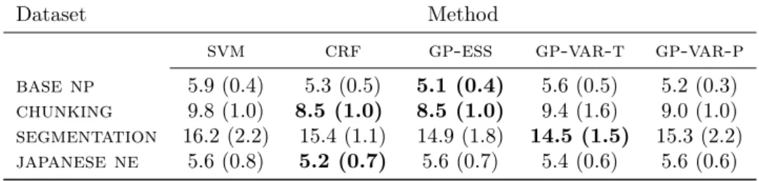
-Table 2: Mean error rates and standard deviations in brackets on small-scale experiments using 5-fold cross-validation. The average number of observed words (N¯) on these problems range from 942 to 3740. svmcorresponds to structured support vector machines; crfto conditional random fields;gp-esscorresponds togpstructwithessfor inference (Bratières et al., 2015); gp-var-tcorresponds to our method with true likelihood; andgp-var-pcorresponds to our our method with piecewise pseudo-likelihood.
Dataset Method
svm crf gp-ess gp-var-t gp-var-p base np 5.9 (0.4) 5.3 (0.5) 5.1 (0.4) 5.6 (0.5) 5.2 (0.3) chunking 9.8 (1.0) 8.5 (1.0) 8.5 (1.0) 9.4 (1.6) 9.0 (1.0) segmentation 16.2 (2.2) 15.4 (1.1) 14.9 (1.8) 14.5 (1.5) 15.3 (2.2) japanese ne 5.6 (0.8) 5.2 (0.7) 5.6 (0.7) 5.4 (0.6) 5.6 (0.6)
Table 3: Negative expected log-likelihoods and standard deviations in brackets on small-scale experiments using 5-fold cross-validation. As before,crfrefers to conditional random fields; gp-esstogpstructwith essfor inference (Bratières et al., 2015);gp-var-t to our method with true likelihood; andgp-var-pto our method with piecewise pseudo-likelihood.
Dataset Method
crf gp-ess gp-var-t gp-var-p base np 944 (835) 887 (57) 622 (34) 603 (21) chunking 517 (113) 704 (116) 407 (43) 587 (100) segmentation 253 (41) 316 (52) 255 (45) 298 (53) japanese ne 592 (131) 806 (135) 339 (38) 411 (94)
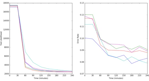
6.3
Larger-scale experiments
Here we evaluate our approach onbase npandchunkingusingNseq= 500training sequences
and the remaining 323 sequences for testing, with a five-fold cross-validation setting. This amounts to roughly11,611training words on average. We compare withcrf, as this was the best baseline in our previous experiments. We also note that that the originalgp-essmethod is completely impractical in this setting.
Onbase np, our method has a lower average test negative log-likelihood (1265.52vs. 1355.63) but a higher error rate (5.15%vs4.50%) thancrf. However, our results onchunking,2511.48
vs1862.96for test log-likelihoods and8.60%vs7.20%for error rates, indicate that our method lags behindcrfon this dataset. We attribute this result tochunkinghaving a much higher dimensionality thanbase np, which is a more critical issue with large datasets, and to the fact that our implementation is not particularly optimized.
6.4
Discussion
As the previous results show, the performance of our variational approach is roughly on par with state-of-the-art methods (and, in particular, consistently better than structured support vector machinessvm) for structured inference over chain models, at least with respect to comparatively small datasets, while being more scalable to the sampling-based implementationgp-ess(which could not be feasibly used for our large-scale experiments).
We cannot claim that our approach is consistently better than custom-made implementations ofcrffor linear chain models; but it is important to remark here that our approach is more
flexiblethan crfin that different choices of likelihood function (e.g. pseudolikelihood rather than true likelihood) can be used without changing anything in the code except the likelihood function itself. This is not the case forcrf: indeed, the likelihood function (computed via the forward-backward algorithm) and its gradients are hard-coded in the used implementation of crf, and changing it would require a substantial reworking of its code.
This is an advantage that our approach shares with the sampling-based approachgp-ess; and, in fact, the present work is in essence an attempt to make said approach more scalable by means of variational and sparse approximation techniques. Overall, the results of our experiments can be considered successful on this note: even though our performance on large-scale experiments was not consistently superior to that ofcrf, as already mentioned our approach is inherently more flexible than it in that it allows to try out different likelihood functions without the need of changing the rest of the implementation.
7
Conclusion
7.1
Future Work
The work discussed in this thesis could be extended in various ways.
First of all, in our experiments we considered only single Gaussians for our variational approximations, even though our approach may be easily extended to Gaussian mixtures. This was because preliminary experiments suggested that increasing the numberK of Gaussians in our variational approximations did not result in improvements for the datasets that we chose to consider; but it would be worthwhile to investigate whether this remains the case when considering other datasets.
The techniques described in this work could also be applied to the problem of image segmentation, extending the work of (Bratières et al., 2014).
Moreover, it could be interesting to explore the benefits of using neural networks to learn the kernels of our Gaussian processes, along the lines of (Hinton and Salakhutdinov, 2008), or even of using variationally approximated structured Gaussian process-based predictors as the last layer of a neural network: in regard to this, the ideas of (Zheng et al., 2015) about the interpretability of Conditional Random Fields in terms of recurrent neural networks could be an intriguing starting point.
Finally, one could study ways of incorporating domain knowledge (in particular, domain knowledge regarding spatial relationships between objects) in our framework. This is a fairly open-ended problem, in general; but for instance, (Hu et al., 2016), in which an expectation maximization-like framework is explored in which a “teacher” network adjusts a “student” network’s prediction by taking into account domain knowledge while the “student” negotiates between the two objectives of fitting the training data and imitating the “teacher” network, could well constitute a very suitable initial point for our exploration.
7.2
Concluding Remarks
We studied a Bayesian structured prediction model withgppriors and linear-chain likelihoods. We developed an automated variational inference algorithm that only requires expectations over low-dimensional Gaussians in order to estimate the expected likelihood term in the variational objective. We exploited these types of theoretical insights as well as practical statistical and optimization tricks to make our inference framework scalable and effective. Our model generalizes recent advances incrfs (Koltun, 2011) by allowing general positive definite kernels defining their energy functions and opens new directions for combining deep learning with structure models (Zheng et al., 2015).
As mentioned in the introduction, when adapting our approach to new structured prediction problems one may need to set up a new configuration of the latent functions (e.g. the unary and pairwise functions of our linear-chain case), which would require substantial modifications to the code. Thus, the process of developing an inference procedure, using our approach, for a different structure (e.g. when considering higher-order interactions) requires some human intervention. Nevertheless, when applied to fixed structures our approach is “black box” with respect to the choice of likelihood, inasmuch as different likelihoods can be used without any change to the inference engine.
We have already seen a possible way to extend our method to more general structured likelihoods, where the exact likelihood is replaced by a piecewise pseudo-likelihood. Such an approach might be especially valuable when adapting our framework to models such as grids or skip-chains, for which the evaluation of the true structured likelihood would be intractable.
Overall, we believe our approach is a fundamental step to developing automated inference methods for general structured prediction problems.
8
Bibliography
Mark Aizerman. Theoretical foundations of the potential function method in pattern recognition learning. Automation and remote control, 25:821–837, 1964.
Mauricio Álvarez and Neil D Lawrence. Sparse convolved Gaussian processes for multi-output regression. InNIPS, pages 57–64. 2009.
Mauricio A Álvarez and Neil D Lawrence. Computationally efficient convolved multiple output Gaussian processes. JMLR, 12(5):1459–1500, 2011.
Mauricio A. Álvarez, David Luengo, Michalis K. Titsias, and Neil D. Lawrence. Efficient multioutput Gaussian processes through variational inducing kernels. InAISTATS, 2010.
Gökhan Bakir. Predicting structured data. MIT press, 2007.
Julian Besag. Statistical analysis of non-lattice data. Journal of the Royal Statistical Society. Series D (The Statistician), 24:179–195, 1975.
David M Blei, Michael I Jordan, and John W Paisley. Variational Bayesian inference with stochastic search. InProceedings of the 29th International Conference on Machine Learning (ICML-12), pages 1367–1374, 2012.
Liefeng Bo and Cristian Sminchisescu. Twin Gaussian processes for structured prediction.International Journal of Computer Vision, 87(1-2):28–52, 2010.
Edwin V. Bonilla, Kian Ming A. Chai, and Christopher K. I. Williams. Multi-task Gaussian process prediction. InNIPS. 2008.
Sébastien Bratières, Novi Quadrianto, Sebastian Nowozin, and Zoubin Ghahramani. Scalable Gaussian process structured prediction for grid factor graph applications. InICML, 2014.
Sébastien Bratières, Novi Quadrianto, and Zoubin Ghahramani. GPstruct: Bayesian structured prediction using Gaussian processes. IEEE TPAMI, 37:1514–1520, 2015.
Don Coppersmith and Shmuel Winograd. Matrix multiplication via arithmetic progressions. In
Proceedings of the nineteenth annual ACM symposium on Theory of computing, pages 1–6. ACM, 1987.
Amir Dezfouli and Edwin V Bonilla. Scalable inference for Gaussian process models with black-box likelihoods. InNIPS. 2015.
Noah D. Goodman, Vikash K. Mansinghka, Daniel M. Roy, Keith Bonawitz, and Joshua B. Tenenbaum. Church: A language for generative models. InUAI, 2008.
Alex Graves et al. Supervised sequence labelling with recurrent neural networks, volume 385. Springer, 2012.