MURDOCH RESEARCH REPOSITORY
Kajornrit, J., Wong, K.W. and Fung, C.C. (2012) A comparative
analysis of soft computing techniques used to estimate missing
precipitation records. In: International Telecommunications
Society 19th Biennial Conference, ITS 2012, 18 - 21 November,
Bangkok, Thailand.
A Comparative Analysis of Soft Computing Techniques
Used to Estimate Missing Precipitation Records
Jesada Kajornrit1, Kok Wai Wong2, Chun Che Fung3
School of Information Technology, Murdoch University South Street, Murdoch, Western Australia, 6150
[email protected], [email protected], [email protected]
Abstract.Estimation of missing precipitation records is one of the most important tasks in hydrological and environmental study. The efficiency of hydrological and environmental models is subject to the completeness of precipitation data. This study compared some basic soft computing techniques, namely, artificial neural network, fuzzy inference system and adaptive neuro-fuzzy inference system as well as the conventional methods to estimate missing monthly rainfall records in the northeast region of Thailand. Four cases studies are selected to evaluate the accuracy of the estimation models. The simultaneous rainfall data from three nearest neighbouring control stations are used to estimate missing records at the target station. The experi-mental results suggested that the adaptive neuro-fuzzy inference system could be considered as a recom-mended technique because it provided the promising estimation results, the estimation mechanism is trans-parent to the users, and do not need prior knowledge to create the model. The results also showed thatfuzzy inference system could provide compatible accuracy to artificial neural network.In addition, artificial neural network must be used with care becausesuch model is sensitive to irregular rainfall events.
Keywords: Missing Precipitation Records, Artificial Neural Network, Fuzzy Inference System, Adaptive Neuro-Fuzzy Inference System, Northeast Region of Thailand
1. Introduction
In hydrological and environmental modelling, precipitation data are one of the most important variables. In Thailand, rain-fall data play the most important role to a variety of hydrological models (streamflow, rainrain-fall-runoff) and environmental models (crop yield estimates, drought risk and severity). These models fundamentally require the complete and reliable rainfall data records. Normally, ground-based observations are the primary source of rainfall data. However, in practice, rainfall records often contain missing data values due to malfunctioning of equipment or human error. Such imperfect rain-fall data could affect the performance of the hydrological and environmental models. Therefore, estimating missing rainrain-fall data is an important task in hydrology [16].
In the last decades, soft computing techniques have been widely adopted in hydrological study. Those techniques could handle the non-linearity and uncertainty in hydrological data. For estimation of missing rainfall data problem, Artificial Neural Network (ANN) and Fuzzy Inference System (FIS) have proved that they provide good estimation accuracy [1][2][8][16][19]. However, those studies just addressed the problem in daily scale. The estimation results may be changed when the data are in monthly scale, in which the variation of data is larger. Furthermore, the estimation result may change according to the study area. In the northeast region of Thailand, the estimation of missing rainfall data has not been studied in depth before. This study provides some study in the use of soft computing techniques to estimate missing monthly rain-fall data in this area.
The paper is organized as follows; Section 2 discusses some issues related to estimation of missing precipitation data problem. Section 3 briefly describes the estimation techniques used in this study. Section 4 illustrates four case studies and section 5 shows experimental results and analysis. The conclusion is presented in section 6.
2. Estimation of Missing Precipitation Data
In general, the estimation of missing precipitation data could be broadly grouped into two types based on the data used to create the estimation models. In the first type, the estimation model is created based on only spatial data. This type of estimation model is usually used for estimating missing precipitation data in the global scale, in which there are a large number of rain gauge stations containing missing data (target stations) that need to be estimated simultaneously [6][7][14]. In the second type, the estimation model is created based on historical data between selected neighbouring stations (control stations) and target stations. This type of estimation model focuses on the local scale wherein a few rain gauge stations are
used in the study. In this type, the estimation model is created by using the relationship of rainfall data between selected controls station and target station from historical records [1][2][9][13][18][19][20]. The study in this paper can be grouped under this type.
The soft computing techniques such as ANN have been widely adopted in variety of hydrological studies [4]. In second type of the estimation of missing rainfall data problem, ANN could be seen as a good alternative method as it provides bet-ter estimation accuracy [8][16][17]. Those models learn the generalized relationship of rainfall data between control sta-tions and target station from historical records. The advantage of ANN is that a model is easy to use and requires no under-standing of the operational details of the model. Furthermore, ANN does not need prior knowledge of the problem.
Teegavarapu et al. [16] mentioned in their comparison work that ANN and Correlation Coefficient Weighting Method (CCWM) could be a recommended technique since these methods provided high estimation accuracy from their study. Coulibaly et al. [2] suggested that among several types of ANN, the multilayer perceptron is suitable for estimating missing daily precipitation values. Kim et al. [8] used ANN to capture the relationship of precipitation from the selected control stations and control station by regression tree technique to estimate the missing data.FIS is another technique that was used to estimate missing precipitation data[1].Even thoughit is not as popular as ANN,the advantage of FIS is that such model is more transparent to the users, however, supplementaryprocedure are needed to create the model.
For studies mentioned above, one can realize that ANN had become the popular technique to solve this problem. How-ever, there is no one method which works well on every dataset. The estimation accuracy may change according to the study area. Furthermore, the more advance technique such as Adaptive Neuro-fuzzy Inference System (ANFIS) has not been investigated to this problem before. Therefore, in order to search for an appropriate method for this study area, com-parison and analysis are necessary. In the next section, the estimation techniques used in this experiment will be discussed.
3. Estimation Techniques
3.1Inverse Distance Weighting Method (IDWM) is an exact interpolation method which estimates the values at unsampled points by using a linear combination of values from nearby sampled points weighted by an inverse distance function. The mathematical formula of IDWM can be expressed as
𝑧𝑜= [ 𝑠𝑖=1𝑧𝑖 1 𝑑𝑖𝑘] [ 1 𝑑𝑖𝑘] 𝑠 𝑖=1 . (1)
where z0 represents the estimated value at location (x0, y0), S is the number of sampled points around the estimated points
and di is the distance between (x0, y0) and (xi, yi), k is a power parameter used for the estimation [16].
3.2 Correlation Coefficient Weighting Method (CCWM) is linear combination of value of neighboring points in which weight are derived from the coefficient of correlation (CC) between any two data sets. Since the coefficient of correlation is one way of quantifying the strength of spatial autocorrelation, it is meaningful to replace the weighting factor by CC [16]. The mathematic formula of CCWM can be expressed as
𝑧𝑜= si=1𝑧𝑖𝜃𝑖 si=1𝜃𝑖 . (2)
wherez0 represents the estimated value at location (x0, y0), S is the number of sampled points around the estimated points
and θiis the correlation coefficient of historical data between the control station and the target station[16].
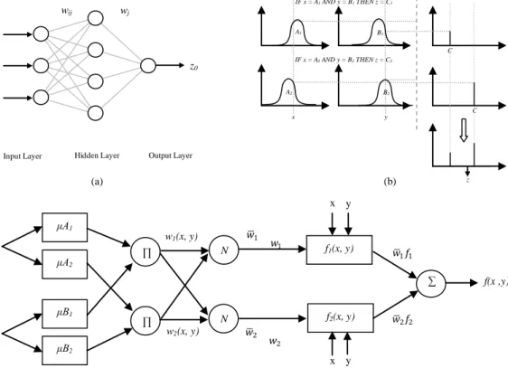
3.3Artificial Neural Network (ANN) is a bio-inspired computing technique for modeling a wide range of nonlinear sys-tem.The high degree of accuracy gained from ANN comes from the parallel processing of information through the net-works of neurons and connected weight [12]. Weights in ANN can be seen as long term memory of the model. In this study, one hidden layer back-propagation neural network (BPNN) is adopted [2]. This architecture has been widely used in hydrology area. The architecture of the BPNN consists of nodes and links connected in consecutive layers. Usually, it can be grouped into three layers, namely, input layer, hidden layer and output layer.
Figure 1a shows an overview of the system architecture of BPNN used in this study. In general, BPNN learns in two ways, the forward propagation and the backward propagation. The forward propagation is used to derive the output from a given inputs. The forward propagation maps inputs into outputby following mathematical representation:
𝑧𝑡 = 𝑤0+ 𝑤𝑗𝑜𝑢𝑡𝜑 𝑤0+ 𝑤𝑖,𝑗𝑧𝑡−𝑖 𝑝
𝑖=1 𝑞
𝑗 =1 . (3)
where wi,j (i = 0, 1, 2,..., p, j = 0, 1, 2, …,q) and wj (j = 0, 1, 2, …,q) are connected weight. p is the number of input nodes;
backward propagation, BPNN adjusts itself according to the training data through the learning algorithm called backward propagation algorithm. The algorithm adjusts weights according to the error that propagates back from output node to input nodes. The backward propagation is used to calibrate model according to training data.
3.4 Fuzzy Inference System (FIS) is a process of mapping from given inputs to outputs by using the theory of fuzzy sets [21]. FIS has been successfully applied in various fields of applications [18][19]. FIS is an appropriate technique to apply into hydrology filed because FIS allows variables to be “partial true” and/or “partial false”, which reflects to the uncertain-ty in physical process. FIS derives an output by using an inference engine which based on a form of IF-THEN rules. Basi-cally, there are two typical approaches to defuzzify fuzzy sets outputs and they are Mamdani[10]and Sugeno[15] approach-es. The Mamdani approach defuzzifies output fuzzy sets by finding the centroid of a two-dimensional shape by integrating across a continuously variation function. In the Sugeno approach, output fuzzy sets are in the form of singleton, a fuzzy set with unity membership grade at a singleton point and zero everywhere else on the universe of discourse. The output centro-id is calculated by the weighted average method. In this study, the Sugeno approach is used because it is computationally efficient, works well with optimization and adaptive techniques and guaranteed continuity of the output surface.An exam-ple of inference process of Sugeno method is shown in Figure 1b.
3.5Adaptive Neuro-Fuzzy Inference System (ANFIS) [5] is similar to Sugeno FIS which is able to adjust its parameters to training data by using back-propagation algorithm. A general structure of ANFIS is shown in Figure 1c (For simplicity in illustration, it was assumed that ANFIS had two inputs, x and y, and one output, z). According to Figure 2, ANFIS consists of five successive layers.Briefly, Layer1 (Input nodes)used to generate membership grades of crisp inputs. Layer2 (Rule nodes) generating firing strengths, which is the product of all the incoming signals. Layer3 (Average nodes)computes the ratio of firing strength of each node ith rule to the sum firing strength of all rules. Layer 4 (Consequence Nodes) computes output according to ith rule toward total output of the model.Layer5(Output nodes) computes the overall crisp output by summing all incoming signals. ANFIS adapts its parameters according to training data by using the hybrid learning algo-rithm. The algorithm consists of the gradient descent for tuning the non-linear antecedent parameters and the least-square for tuning linear consequent parameters.
(a) (b)
(c)
Figure 1: An overview of system architecture of (a) back-propagation artificial neural network, (b) Sugeno-type fuzzy inference system,
(c) Adaptive neuro-fuzzy inference system.
Hidden Layer Output Layer
z0 wj wij Input Layer z1 z2 z3 μA1 μA2 μB1 μB2 f1(x, y) ∏ ∏ N N f2(x, y) x y w1(x, y) w2(x, y) 𝑤1 = 𝑤1 𝑤1+ 𝑤2 𝑤2 = 𝑤2 𝑤1+ 𝑤2 𝑤1𝑓1 𝑤2𝑓2 f(x ,y)
Layer 1 Layer 2 Layer 3 Layer 4 Layer 5
x y x y ∑ x y A1 A2 B2 B1 IF x = A1 AND y = B1 THEN z = C1 IF x = A2 AND y = B2 THEN z = C2 C 2 C 1 z
4. Four case studies and datasets
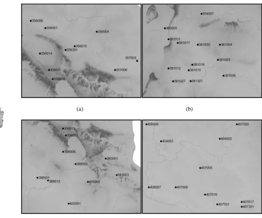
The northeast region of Thailand can be seen as the biggest part of Thailand. The area covers one third of total area of the country. Figure 3 illustrates the study area. In this study, four rainfall stations are used to validate the models. These stations are assumed to have missing rainfall data records (target station). Many researchers recommended the use of three or four closest stations for application of IDWM [16]. This suggestion was confirmed by the work of [3]. They showed that inclusion of more than four stations does not significantly improve the interpolation and may in fact degrade the estimation results. This study therefore selected three closest neighboring observations (control station) to estimate missing data at target station. Another reason for this selection is due to the availability of data. Unfortunately, since the dataset contain the real missing data in the early period, the data records that have missing data must be removed. The number of available data records decreases when the number of control stations increases. Thus, the use of three control stations could be an appropriate selection.
The rainfall data used was range from 1981 to 2001. The data from 1981 to 1998 were used to calibrate the models and data from 1999 to 2001 were used to validate the developed models. Since there are a few real missing data records from control stations in earlier period, such record must be removed. After removing missing records from calibration data, the proportion between validation and calibration data falls between18 to 20 percents approximately. To validate the models, Mean Absolute Error (MAE) is adopted as given in equation (4).
𝑀𝐴𝐸 = 𝑚 𝑂𝑖 − 𝑃𝑖
𝑖=1 𝑚 . (4)
where Oi and Pi is the observed the estimated value respectively, m is the number of missing data. The statistics of data in
this case study are shown in Table 1
(a) (b)
(c) (d)
Figure 3: Four selected rain-gauged stations used in this study are from the northeast region of Thailand, (a) case 1: ST356010, (b) case
2: ST381010, (c) case 3: ST388002, (d) case 4: ST407005. Case 1 and case 3 sites are located over and under the Phu-Phan Mountains Range respectively. Case 2 site is located in the Northern Sakon-Nakhon plain and case 4 site is located s in the Southern Khorat plain.
1 2 3 4 Thailand N
Southern Khorat plain
Phu-Phan mountain range
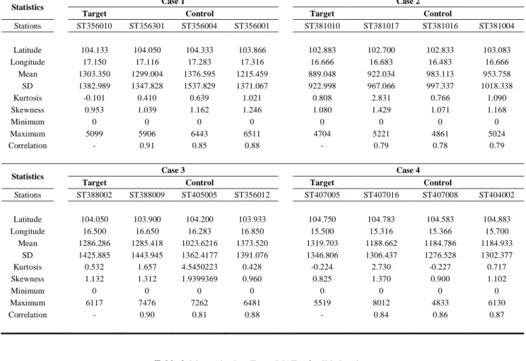
Table 1. Statistics of rainfall data in thefour case studies
Statistics Case 1 Case 2
Target Control Target Control
Stations ST356010 ST356301 ST356004 ST356001 ST381010 ST381017 ST381016 ST381004 Latitude 104.133 104.050 104.333 103.866 102.883 102.700 102.833 103.083 Longitude 17.150 17.116 17.283 17.316 16.666 16.683 16.483 16.666 Mean 1303.350 1299.004 1376.595 1215.459 889.048 922.034 983.113 953.758 SD 1382.989 1347.828 1537.829 1371.067 922.998 967.066 997.337 1018.338 Kurtosis -0.101 0.410 0.639 1.021 0.808 2.831 0.766 1.090 Skewness 0.953 1.039 1.162 1.246 1.080 1.429 1.071 1.168 Minimum 0 0 0 0 0 0 0 0 Maximum 5099 5906 6443 6511 4704 5221 4861 5024 Correlation - 0.91 0.85 0.88 - 0.79 0.78 0.79
Statistics Case 3 Case 4
Target Control Target Control
Stations ST388002 ST388009 ST405005 ST356012 ST407005 ST407016 ST407008 ST404002 Latitude 104.050 103.900 104.200 103.933 104.750 104.783 104.583 104.883 Longitude 16.500 16.650 16.283 16.850 15.500 15.316 15.366 15.700 Mean 1286.286 1285.418 1023.6216 1373.520 1319.703 1188.662 1184.786 1184.933 SD 1425.885 1443.945 1362.4177 1391.076 1346.806 1306.437 1276.528 1302.377 Kurtosis 0.532 1.657 4.5450223 0.428 -0.224 2.730 -0.227 0.717 Skewness 1.132 1.312 1.9399369 0.960 0.825 1.370 0.900 1.102 Minimum 0 0 0 0 0 0 0 0 Maximum 6117 7476 7262 6481 5519 8012 4833 6130 Correlation - 0.90 0.81 0.88 - 0.84 0.86 0.87
Table 2. Mean Absolute Error (MAE) of validation data
Method Case 1 Case 2 Case 3 Case 4
IDWM 245 267 500 399
CCWM 261 285 484 399
BPNN 244 258 487 481
FIS 247 239 484 413
ANFIS 243 236 475 402
5. Experimental Results and Analysis
This section reports the experimental results and presents some analysis discussions. Table 2 shows MAE measures of the validation data. In IDWM, the optimized power parameter k could be defined by considering MAE of data in the cali-bration period when increasing power parameter. Figure 4 shows MAE of calicali-bration data when power parameter increas-es. According to Figure 4, the optimized power parameters are 0.8, 4.5, 2.8 and 0 for case 1 to case 4 respectively. In CCWM, the correlation coefficient between each control stations and target station used in this method are shown in Table 1.
In the work of [16], they recommended to use the CCWM instead of IDWM since it provided better estimation accu-racy. However, in this study, CCWM seems not much improvement from IDWM since it did not show better accuracy than IDWM overall. One plausible reason is that the condition of higher accuracy gained from CCWM depends on the fact that the correlations used must reflect the exact relationship between control station and target station. This condition is proba-bly consistent when it is used for precipitation data in daily scale in which the numbers of training data are quite large and have small variation. In this study, the number of training data is relatively small and variation of data in monthly scale is considerably large. Then, the use of CCWM for estimating missing data may not be an effective way for this case.
Figure 4. Mean Absolute Error (MAE) of data in calibration period when power parameter k is increased. The optimized power parame-ters are 0.8, 4.5, 2.8 and 0 for case 1 to case 4 respectively.
In addition to CCWM, BPNN is another alternativeto estimate missing data suggested by the work of [8]and[16]. The advantage of BPNN model is that BPNN can adapt itself to training data through their learning algorithm. Such model is easy to use model and does not require any prior knowledge. In this study one hidden layer back-propagation neural net-work is adopted. The number of input node is three and the number of output node is one. By trial and error procedure, the numbers of optimized hidden nodes are three or four. The more number of hidden nodes could providelower estimation accuracy. It isbecause the large number of hidden nodes (or parameters) requires a large number of training data [5].In this case, the number of training data is considered small. Such amount of data could not be enough to optimize all parameters in the large BPNN.
From Table 2, BPNN showed almost similar estimation accuracy when compare to IDWM in case 1. In case 2 and case 3, BPNN provided slightly improved estimation accuracy from IDMW. In case 4, however, BPNN provided large estima-tion error. Therefore, some investigaestima-tion into the dataset of case 4 is needed. It was found that there are some rainfall records in the calibration period where the relationship of control stations and target stations could be considered as irregu-lar events. For example, there is an overshoot of rainfall record at target station whereas rainfall data at control stations are normal. If such record occurred frequently in training data, BPNN could not provide good estimation. However, only BPNN is affected by this irregular event becauseBPNN used this record as input-output pair in the training process whereas the IDWM and CCWM do not use the output. This study suggests removing this record before training the BPNN. If poss-ible, expert should be consulted before removing. Even though the accuracy of BPNN did not improve much from IDMW, the ease to use of BPNN is still interesting because noprior knowledge of datasets is needed.
The next soft computing technique is FIS. The FIS in this study are created by subtractive clustering technique. One pa-rameter has to be defined in creating the FIS is a vector that specifies a cluster center's range of influence in each of the data dimensions (or “radii”), assuming the data falls within a unit hyper box. The best values for radii are usually between 0.2 and 0.5[11]. This study adopted radii = 0.5 because the range of MFs created cover all period of data, which results in more accurate than using radii = 0.2. Another reason is that the numbers of clusters generated are two and four when radii = 0.5 and 0.2 respectively. radii = 0.2 is more suitable to be optimized in the ANFIS model because it does not have too many parameters to be tuned when the number of dataset are considered small. The center of the first cluster close to 0 and center of the second cluster fall near to 0.3 as shown in Figure 5a. The number of fuzzy rules generated is two according to the number of clusters.
(a) (b)
Figure 5. An example of membershipfunctions of fuzzy inference system created by subtractive algorithm, (a) membership functions
before optimizing (b) membership functions after optimizing.
0 1 2 3 4 5 300 310 320 330 340 350 360 370 380 390 400 Power degree (k) M e a n A b so lu te E rr o r case 1 case 2 case 3 case 4 0 0.1 0.2 0.3 0.4 0.5 0.6 0.7 0.8 0.9 1 0 0.2 0.4 0.6 0.8 1 in1 D e g re e o f m e m b e rsh ip in1cluster1 in1cluster2 0 0.1 0.2 0.3 0.4 0.5 0.6 0.7 0.8 0.9 1 0 0.2 0.4 0.6 0.8 1 in1 D e g re e o f m e m b e rsh ip in1cluster1 in1cluster2
According to Table 2, FIS provided almost similar estimation accuracy to BPNN in case 1 and case 3. However, the ac-curacy of FIS is better than BPNN in case 2 and case 4.In case 4, FIS reduces the estimation error provided by BPNN out-standingly. It seems that FIS can tolerate to irregular events more than BPNN. Although both BPNN and FIS need no prior knowledge to create the model, FIS is more transparent to the users than BPNN. As fuzzy rules are closer to human reason-ing, an analyst could understand how the model performs the estimation. If necessary, the analyst could also make use of his/her knowledge to modify the estimation model [19]. Taking this point into account, it seems that FIS should be more appropriate than BPNN to perform this task.
The last soft computing technique is ANFIS. An example of optimized MF is shown in Figure 5b. The optimization me-thod expanded the right flank of the left MF. One can see that the FIS in the prevision discussion is the original FIS whe-reas the ANFIS is the optimized FIS. Considering MAE in table 2, ANFIS showed slightly improved estimation accuracy from FIS overall. Even though ANFIS did not show any large improvement from FIS in case 1 and case 2, it provides moderately improvement in case 3 and case 4.In this study, ANFIS could be considered as the most appropriate model among all soft computing techniques because ANFIS provided lowest estimation error in all cases. Furthermore, such model need no prior knowledge as same as BPNN and FIS. Furthermore, the estimation mechanism of ANFIS is the same as FIS, which is transparent to the users.
So far, the experimental results have been discussed. The advantage and disadvantage of every method has been pointed out. Based on this study, one question may rise. Why are the FIS and ANFIS model able to improve the estimation accuracy? The possible reason is that FIS and ANFIS’s mechanism consists of two MFs, in which one captures dry period and another one captures wet period. If the uncertainty of rainfall period is captured well by these MFs, it possible that the heterogeneity of rainfall data may consist of two groups by nature. Therefore, why do we not address this problem by the use of modular models? It may improve estimation accuracy than one single model.
6.Conclusions
This study compared the common-used soft computing techniques as well as conventional methods to estimate monthly missing precipitation records. Four case studies in the northeast region of Thailand are used to evaluate the estimation accu-racy of those models. Overall, the experimental results pointed out that
Firstly, CCWM may not be appropriate to be used for monthly precipitation data prediction as the correlation measure used in CCWM could not exactly reflect the strength of the relationship between the control stations and the target station. Secondly, BPNN could be seen as an alternative technique because it showed slight improvement over IDWM and it does not need prior knowledge to create the model. However, BPNN must be used with care because such model is sensitive to irregular rainfall events.
Next, FIS is more appropriate technique than BPNN to perform this task in term of interpretability. Even though the estima-tion accuracy of BPNN and FIS is not much difference, the estimaestima-tion mechanism of FIS is more transparent to human ana-lysts than BPNN. And human can add in knowledge and modify the prediction model.
Finally, ANFIS could be considered as a recommended technique to other methods because it provided better estimation than BPNN and FIS, Furthermore, the estimation mechanism is transparent to the users, and do not need prior knowledge to create the model.
References
1. Abebe, A.J., Solomatine, D.P., Venneker, R.G.W.: Application of Adaptive Fuzzy Rule-based Models for Reconstruction of Miss-ing Precipitation Events.Hydrological Sciences-Journal-des Sciences Hydrologiques45(3), 425-436 (2000)
2. Coulibaly, P. Evora. N.D.: Comparison of Neural Network Methods for Infilling Missing Daily Weather Records. Journal of Hy-drology 341, 27-41 (2007)
3. Eischeid, J.K., Pasteris, P.A., Diaz, H.F., Plantico, M.S., Lott, N.J. Creating a Serially Complete, National Daily Time Seri es of Temperature and Precipitation for the Western United States. Journal of Applied Meteorology 39, 1580-1591 (1999)
4. Govindaraju, R.S., Rao, A.R.: Artificial Neural Networks in Hydrology (Water Science and Technology Library), Kluwer Academ-ic Publishers, Netherlands, (2000)
5. Jang, J.S.R., Sun, C.T., Mizutani, E.: Neuro-fuzzy and Soft Computing a Computational Approach to Learning and Machine Intelli-gence. Prentice Hall Inc, Upper Saddle River (1997)
6. Jeffrey, S.J., Carter, J.O., Moodie, K.B., Beswick, A.R.: Using Spatial Interpolation to Construct a Comprehensive Archive of Aus-tralian Climate Data. Environmental Modelling and Software 16, 309-330 (2001)
7. Kajornrit J., Wong, K.W., Fung, C.C.:Estimation of Missing Rainfall Data in Northeast Region of Thailand using Spatial Interp ola-tion Methods. Australian Journal of Intelligent Informaola-tion Processing Systems 13(1), 21-30 (2011)
8. Kim, J., Pachepsky, Y.A.: Reconstructing Missing Daily Precipitation Data Using Regression Trees and Artificial Neural Networks for SWAT Streamflow Simulation. Journal of Hydrology 394, 305-314 (2010)
9. Makhuvha,T., Pegram, G., Sparks R., Zucchini, W.: Patching Rainfall Data Using Regression Methods. 1. Best Subset Selection, EM and Pseudo-EM Methods: theory and 2. Comparisons of accuracy, bias and efficiency, Journal of Hydrology 198, 289–318 (1997)
10. Mamdani, E.H., Assilian, S.: An Experiment in Linguistic Synthesis with Fuzzy Logic Controller. International Journal of Man -machine Studies 7(1), 1-13 (1975)
11. MATLAB®: Fuzzy Logic ToolboxTM 2 User’s guide, MathWorks Inc. (2010)
12. Negnevitsky, M.: Artificial Intelligence a Guide to Intelligence Systems Second Edition. Pearson Education, London (2005). 13. Pegram, G.: Patching Rainfall Data Using Regression Methods. 3. Grouping, Patching and Outlier Detection. Journal of Hydrology
198, 319–334 (1997)
14. Piazza, A.D., Conti, F.L., Noto, L.V., Viola, F., Loggia, G.L.: Comparative Analysis of Different Techniques for Spatial Interpola-tion of Rainfall Data to Create a Serially Complete Monthly Time Series of PrecipitaInterpola-tion for Sicily, Italy. InternaInterpola-tional Journal of Applied Earth Observation and Geoinformation 13, 396–408 (2011)
15. Sugeno, M.: Industrial Application of Fuzzy Control. North-Holland, Amsterdam (1985)
16. Teegavarapu, R.S.V., Chandramouli, V.: Improved Weighting Methods, Deterministic and Stochastic Data-Driven Models for Es-timation of Missing Precipitation Records. Journal of Hydrology 312, 191-206 (2005)
17. Teegavarapu, R.S.V., Tufail, M., Ormsbee, L.: Optimal Functional Forms for Estimation of Missing Precipitation Data. Journal of Hydrology 374, 106–115 (2009)
18. Wong, K.W., Gedeon, T.D.: Petrophysical Properties Prediction using Self-generating Fuzzy Rules Inference System with Modified Alpha-cut Based Fuzzy Interpolation. In: The 7th International Conference of Neural Information Processing, pp. 1088-1092. IEEE Press, Korea (2000)
19. Wong, K.W., Wong, P.M., Gedeon, T.D., Fung, C.C.: Rainfall Prediction Model using Soft Computing Technique. Soft Computing Vol. 7, No. 6, 434-438, Springer, (2003)
20. Xia, Y., Fabian, P., Stohl, A., Winterhalter, M.: Forest Climatology: Estimation of Missing Values for Bavaria, Germany. Agricul-tural and Forest Meteorology 96, 131-144 (1999)