Analyzing Graph Databases by Aggregate Queries
Anton Dries
Siegfried Nijssen
K.U.Leuven, Celestijnenlaan 200A, Leuven, Belgium
{anton.dries,siegfried.nijssen}@cs.kuleuven.be
ABSTRACT
An important step in data analysis is the exploration of data. For traditional relational databases one of the most powerful tools for performing such analysis is the relational database and the aggregates and rankings that they can compute: for instance, simple statistics such as the average number of links between two types of entities (relations) are easily computed using a query on a relational database and may already provide valuable information. However, for the ex-ploration of graph data, relational databases may not be most practical and scalable. For instance, a statistic such as the shortest path between two given nodes cannot be com-puted by a relational database. Surprisingly, however, tools for querying graph and network databases are much less well developed than for relational data, and only recently an increasing number of studies are devoted to graph or network databases. Our position is that the development of such graph databases is important both to make basic graph mining easier and to prepare data for more complex types of analysis. An important component of such databases is the language that is used to enable aggregating queries, such as shortest path queries.In this paper, we propose an extension to a previously proposed query language. This extension allows for querying and analyzing databases by using ag-gregates and ranking. A notable feature of our language is that it also supports probabilistic graph queries by conceiv-ing of such queries as aggregatconceiv-ing queries. We demonstrate its value on a simple data analysis task.
Categories and Subject Descriptors
H.2.1 [Database Management]: Logical Design—Data Models
General Terms
Design, TheoryPermission to make digital or hard copies of all or part of this work for personal or classroom use is granted without fee provided that copies are not made or distributed for profit or commercial advantage and that copies bear this notice and the full citation on the first page. To copy otherwise, to republish, to post on servers or to redistribute to lists, requires prior specific permission and/or a fee.
MLG’10,July 24-25, 2010, Washington DC, U.S.A. Copyright 2010 ACM I978-1-4503-0214-2/10/07 ...$10.00.
Keywords
Graph databases, Inductive databases, Data mining
1.
INTRODUCTION
Even though one can have doubts whether database sys-tems can be called data mining syssys-tems, in practice database systems are often used for basic analysis and preparation of relational data, such as computing aggregates or histograms of attributes, ranking tuples, or even computing the number of links to a certain tuple in a table [9]. Such basic analysis is often important to gain an initial impression of data and understand the main distributions of attributes in data; in many cases already interesting knowledge can be obtained by only such basic querying.
Considering that this is the case for relational data, the motivation for the work in this paper is that this may also be true for graph data. In many applications it is increasingly common to represent data as a large graph or network: ex-amples include social networks, bibliographic networks and biological networks. Modeling the data as graphs is conve-nient in these applications as traditional graph-based con-cepts, such as paths, cliques, node degrees, edge degrees, and so on, are useful in their analysis. However, traditional rela-tional database systems do not support these concepts and hence can only be used for very limited types of graph anal-ysis, which raises the question how one can build databases that support these concepts.
The interest in integrating graphs in database systems has led to several recent proposals for graph query languages [7, 23, 10, 13, 8, 14, 20], which support basic concepts such as nodes, edges and paths between nodes. A distinguishing fea-ture of graph query languages is that they allow for declar-ative querying: they allow a user to specify whichpiece of information to find instead ofhowto find this. Even though declarative querying may not yield the most scalable solu-tions for specific tasks, a good declarative language enables more users to express problems in such a way that automatic systems find solutions within reasonable time.
When we consider the history of database technology, one of the early popular data models was the network data model. To access data in the network model, the CODASYL data management language was developed. CODASYL was a low-level language in which a user was required to specify the paths along which to access data; for instance, it con-tained a NEXT statement to move to the next element of a linked list. The relational model became more popular due to its higher level of abstraction; it allowed user to specify what they want to find and to no longer consider how to
find it.
The state-of-the-art in how machine learning and data mining deal with graphs and networks is in some ways sim-ilar to these early days of database research. Database sys-tems [18] as well as specialized graph libraries in host lan-guages such as Java or C++ [19, 17] do not provide a declar-ative querying interface but rather rely on lower-level princi-ples such as graph traversers. To the best of our knowledge, a more declarative query language which supports aggregat-ing queries does not currently exist.
Another recent development is that of probabilistic data-bases. In a probabilistic database tuples or entries are no longer strictly true or false, but are only true or false to a certain degree; consequently, the results of queries may also only be true to a certain degree. Recently, approaches based on logic programming have been developed that allow for the formulation of probabilistic logic queries on proba-bilistic logic databases. An interesting direction of research is to merge such approaches with graph databases; ideally a query language supports such integration, even if currently no underlying database management system exists that can answer such queries on a large scale.
The problem that we hence study in this paper is the de-velopment of a declarative query language supporting basic graph analysis and data preparation tasks. In our opinion, key features that such a database should support are:
• it should support graph-based concepts, such as paths and node connectivity;
• it should support aggregates, ranging from simple ones (such as node degrees) to more complex ones (such as path length or even path probability in probabilistic networks);
• it should support ranking, in order to filter results of less interest.
In previous work we proposed a declarative query language, called BiQL, for posing queries in a graph database. This language included primitives which allowed for basic data transformation steps. Such steps can be important when preparing a database for analysis by a more complex algo-rithm, for instance, algorithms for finding important nodes [4, 22], important connections [22], or methods for classify-ing [22] or clusterclassify-ing nodes [12]. The inclusion of aggregate queries, needed for basic types of analysis and converting databases in weighted or probabilistic graphs, was left as future work. In this paper, we provide the details of an ex-tension of our language towards aggregates, and we discuss how to (conceptually) evaluate such queries.
The outline of this paper is as follows. In Section 2 we summarize the motivations that led to the development of the core BiQL data model and query language. Section 3 introduces related work. In Section 4 we summarize our data model and the basic query language. Section 5 introduces the extension towards aggregates and ranking. In Section 6 we illustrate how our system can be used on a showcase application. In Section 7 we conclude.
2.
REQUIREMENTS
The main motivation and target application for our data model and query language, as presented in [6], is support-ing exploratory data analysis on networked data. Below we summarize the requirements and design choices.
Small is beautiful. The data model should consist of a small number of concepts and primitives. As a consequence, we do not wish to introduce special language constructs to deal with complicated types of networks (directed, undirected, labeled, hypergraphs, etc.) or sets of graphs.
Uniform representation of nodes and edges. The most im-mediate consequence of the former choice is that we wish edges and nodes to be represented in a uniform way. We will do this by representing both edges and nodes as ob-jects that are linked together by links that have no specific semantics. This also allows one to generate different views on a network. For instance, in a bibliographic database, we may have objects such as papers, authors and citations. In one context one could analyze the co-author relationship, in which case the authors are viewed as nodes and the papers as edges, while in another context, one could be more inter-ested in citation-analysis, in which case the papers are the nodes and the citations the edges.
Closure property. The result of any operation or query can be used as the starting point for further queries and oper-ations. The information created by a query combined with the original database can therefore be queried again.
SQL-based. There are many possible languages that could be taken as starting point, such as SQL, relational algebra or Datalog. We aimed for a data model on which multiple equivalent ways to represent queries can be envisioned. The queries that we propose on this model are expressed in an SQL-like notation here, as this notation is more familiar to many users of databases, and is the prime example of a declarative query language.
In addition to these requirements, in this paper we identify the following requirements.
Aggregates. To support a basic analysis of graphs, we need to be able to calculate statistics such as
• the degree of nodes;
• the number of nodes reachable from a certain node (connected component size);
• the length of a shortest path between two nodes;
• the length of the longest shortest path from one node to all other nodes (node centrality);
• the sum or product of weights on edges on paths. These statistics are not only useful when obtaining an initial insight in data. It is also important that these statistics can be inserted when a new graph is generated (representing an-other context). For instance, in simple random walk models the probability of going from one node to another node may be determined by the degrees of the nodes involved. These probabilities can be seen as attributes of the edges; ideally, a database query would be sufficient to put these probabilities in a graph. The closure property entails that we can also run queries on the attributes generated in this way. One such type of query could be aprobabilisticquery, which calculates new probabilities from probabilities present in the network.
Ranking. Once an aggregate is computed, it can be desirable to rank results on aggregate values; for instance, one may not be interested in the centrality of all nodes, but only in the nodes that are most central. A database system should support such ranking queries and ideally be optimized to an-swer them more efficiently than by post-processing a sorted list of all results.
3.
RELATED WORK
In this section we provide a more detailed discussion of re-lated work, which makes clear the limitations of the current systems and languages.
Graph Query Languages. A number of query languages for graph databases have been proposed, many of which have been described in a recent survey [2]. GraphDB [7] and GOQL [23] are based on an object-oriented data model, with specific, separate types of objects for use in networks such as nodes, edges and paths. Both languages devote a lot of attention to querying and manipulating paths: for example, GraphDB supports regular expressions and path rewriting.
GraphQL [10] provides a query language that is based on graph patterns. In this model graphs are a basic unit; the language is geared towards finding occurrences of small graphs in both large sets of small graphs as well as small sets of large graphs. Edges and nodes are treated separately; it has no support for paths or aggregates.
PQL [13] is an SQL-based query language which has added support for treating paths as objects; It does not provide functionality for adding new nodes in a network or aggre-gating queries.
GOOD [8] was one of the first systems that used graphs as its underlying representation. Its main focus was on the development of a database system that could be used in a graphical interface. To this end it defines a graphical transformation language, which provides limited support for graph pattern queries. This system forms the basis of a large group of other graph-oriented object data models such as Gram [1] and GDM [11].
Hypernode [14] and GROOVY [15] use a representation based on hypernodes, which make it possible to embed a graph as a node in another graph. This recursive nature makes them very well suited for representing arbitrarily com-plex objects, but also makes the model more comcom-plex than necessary for analyzing most networks in data mining.
More recently, approaches based on XML and RDF such as SPARQL [20], are being developed. SPARQL aims at extracting information from RDF data, where edges do not have attributes and express relationships between nodes. It is not focused on network data with multiple types of entities and does not provide extensive support for adding nodes to a network or aggregation.
Graph Databases. Whereas the previous studies propose declarative query languages, recently several storage systems have been proposed that do not provide a declarative query language. Notable examples here are Neo4J [18] and DEX [16], which provide Java interfaces to graphs persistently stored on disk. For Neo4J an alternative programming lan-guage called Gremlin is under development [21].
Graph Libraries.Finally, in some communities Java or C++ libraries are used for manipulating graphs in the memory of the computer (as opposed to the above graph databases which support typical database concepts such as transac-tions). Examples are SNAP [19] and igraph [17].
4.
BASIC DATA MODEL
Our data model consists of several parts: (1) thestructural partof the data model; (2) themanipulation partof the data model; (3) theintegrity partof the data model. We will here summarize the basic elements involved in (1) and (2); for details on data integrity see [6].
obj-id features X1 {label=A, color=red} X2 {label=B, color=yellow} X3 {label=C, color=blue} X4 {label=D, color=yellow} X5 {label=E, color=red} Y1 {weight=0.2} Y2 {weight=0.5} Y3 {weight=0.8} Y4 {weight=0.2} Y5 {weight=0.9}
(a) Object store
Y1 ↔ X1 Y1 ↔ X2 Y2 ↔ X1 Y2 ↔ X3 Y3 ↔ X2 Y3 ↔ X3 Y4 ↔ X3 Y4 ↔ X4 Y5 ↔ X3 Y5 ↔ X5 (b) Link store
name objects Comment
X {X1, X2, X3, X4, X5} Nodes
Y {Y1, Y2, Y3, Y4, Y5} Edges
(c) Domain store Table 1: Example database
4.1
Data Structures
Our data structure consists of the following components. The object store, which contains all objects in a data-base. Objects are uniquely identified by an object identifier. Each object can contain an arbitrary list of attribute-value pairs describing its features. The link store, which contains directed links between
ob-jects. They can be represented as (ordered) pairs of object identifiers, and do not have any attributes. The domain store, which contains named sets of objects.
A domain name allows users to identify a set of objects. The main design choice in this data structure is to not allow attributes on links. Between every pair of objects a link may or may not exist. We do not specify how links are stored. A basic operation is to check if a link exists between two objects.
Domains are used to group nodes of a certain type to-gether. In a bibliographic database, groups of nodes may be
authorsorpapers. One may think of the objects as nodes in a graph, and of the links as unlabeled binary edges be-tween these nodes. However, this raises the question how we represent edge labeled graphs or hypergraphs. This is clarified in the following example.
Example 1 (Edge Labeled Graph). Assume given the objects and links in Table 1, belonging to domainsX and
Y, together constituting the graphG. Then we can visualize
G as given in Figure 1. In this example, one may think of nodes A, ..., E as authors, and as the edges expressing strengths of co-authorships.
Hence, the main choice that we have made is that also edges are represented as objects. An edge object is linked to the nodes it connects. Even though this may not seem intu-itive, or could seem a bloated representation, the advantages of this choice outweigh the disadvantages because:
• by treating both edges and nodes as objects, we obtain simplicity and uniformity in dealing with attributes;
• it is straightforward to treat (hyper)edges as nodes (or nodes as (hyper)edges);
0.2 0.9 0.8 0.5 0.2 A D E B C
Figure 1: A visualization of context G in the example da-tabase in Table 1, where we use domain X as nodes and domainY as edges. 0.8 0.5 0.9 B A C D E
Figure 2: View on the database using the new table Y’.
• it is straightforward to link two edges, for instance, when one wishes to express a similarity relationship between two edges.
4.2
Data Manipulation
In this section we introduce the main components of the BiQL query language, which allows for basic (deductive) querying using an SQL-like notation. The extensions needed to deal with aggregates and ranking will be discussed in the next section.
In general a query looks like this.
CREATE <domain name> AS
SELECT <definitions of domains>
FROM <selection from domains>
WHERE <predicate on attributes of objects> A simple example of such a query is this:
CREATE Y’ AS SELECT E FROM Y E
WHERE E.weight > 0.4
This statement creates a new domain Y0; the objects that are inserted in this domain are obtained by letting a variable
Erange over the objects in domainY; those objects which have a weight attribute with a value higher than 0.4 are inserted.
ForY defined as in Table 1, the resulting domain contains the following set of identifiers.
Y0={Y2, Y3, Y5}
We can define a new graph, visualized in Figure 2, by using
X as nodes andY0 as edges (Figure 1).
Below we provide some more details on the FROM,WHERE
andSELECTparts of a query; see also [6] for more details.
4.2.1
WHEREstatement
In theWHEREstatement constraints are expressed based on the features of the objects that the variables refer to. These constraints are similar to those in SQL, and include compar-isons of attributes of objects and compositions thereof into formulas using ANDs and ORs.
Figure 3: A simple graph pattern
4.2.2
FROMstatement
An important distinguishing feature is the FROM state-ment. In our language we can usepath expressionsto specify structural constraints on the variables. A simple example of a query, which can be applied on the data in Table 1 is:
CREATE E’ SELECT E FROM X N -- Y E
WHERE E.weight >= 0.9 AND N.color=blue
This statement creates a new domain E’ containing those edge objects that are linked to a blue node object.
In general theFROMstatement consists of a list of path ex-pressions. The simplest form of a path expression consists of a series of domain identifiers separated by the--or->or
<-operators, which represent structural constraints requiring the presence of links in any direction or the presence of links in a given direction.
Conceptually, for every combination of variable assign-ments a tuple of objects (or object tuple) is created. Each element in a tuple is uniquely identified by the name of a variable; only those tuples are selected which satisfy the structural constraints. In our example, one such tuple is
(N:X3,E:Y5). If we letRdenote a set tuples, we can denote a selection by σP(R) in analogy to the relational model,
where P expresses the connectivity conditions that should be satisfied by the elements in a tuple.
Variables can occur multiple times in path expressions by prefixing all but one occurrence with a #. Using this notation, also more complex patterns than paths can be ex-pressed. Consider the followingFROMandWHERE statement:
FROM X N1 -- Y -- X N2 -- Y -- X N3,
#N2 -- Y -- X N4
WHERE N1.color = red AND N2.color = blue
AND N3.color = yellow AND N4.color = black
One can visualize this path expression, together with the
WHEREstatement, as the graph in Figure 3.
4.2.3
SELECTstatement
The SELECT statement expresses which variables in the query are used to define a new domain. In our previous examples, queries always returned subsets of objects of ex-isting domains. However, it can often be useful to create new objects. We illustrate this using the following query.
CREATE PatZ AS
SELECT <N1,E1,N2,E2,N3> {E1->,E2->} FROM X N1 -- Y E1 -- X N2 -- Y E2 -- X N3 WHERE N1.color = red
AND N2.color = blue AND N3.color = yellow
The angle brackets (<...>) express a grouping operation; for each objects tuple (N1,E1,N2,E2,N3) for which the path expression matches the data, a new object is created. This object is linked to objectsE1andE2. Essentially, each object in the result represents an occurrence of a given subgraph.
It is important to note here that the SELECT statement does not need to contain all variables mentioned in theWHERE
statement. If some variables are missing, the object tuples areprojectedon the variables mentioned in theSELECT state-ment; in analogy to projection in relational databases, ifR
denotes a set of tuples,πV(R) removes those elements from
all tuples inR not corresponding to variables listed inV. Hereset semantics are applied, i.e. after projection dupli-cate occurrences of the same tuple are removed. Simple attributes can be assigned to new objects as follows:
SELECT <E>{E.*, weight: E.weight/2} FROM Y E
WHERE E.weight > 0.4
which copies all the attributes from the original object but replaces the weight attribute by its old value divided by two. If the<...>brackets are missing, new attributes can be added to existing objects. It is important to note that between the braces{...}only variables can be used that oc-cur within the grouping brackets<...>: the other variables may have different values in the tuples that were merged together in the projection. To assign additional values to new objects based on sets of tuples, aggregates can be used. This is discussed in the next section.
5.
EXTENDED QUERY LANGUAGE
In this section we will introduce the extensions to our lan-guage step by step. We will first discuss a basic extension with aggregates, followed by a discussion of how to deal with arbitrary regular expressions. We will subsequently extend our language with ranking and will illustrate the overall pro-cedure by which queries are (conceptually) answered.
5.1
Aggregates
The two main types of aggregates arecountand attribute-based aggregates (sum, avg, min, max,. . .). The syntax of an aggregate is illustrated by the following query:
SELECT <N> {weight: sum<E>(E.weight)} FROM X N -- Y E -- X N2
This query determines a weight for nodes; the weight is com-puted by summing the weights of connecting edges. Intu-itively in this query object tuples are first partitioned on the values for N and subsequently further partitioned on the values forE. In the partitioning onN, all tuples within one partition share the same object value forN; in the par-titioning onN andE, all tuples within one partition share the sameN andEvalue. For every value ofN (correspond-ing to a partition of tuples), the aggregate now sums the weights of the E objects in its partition (hence projecting theN2 variable away).
In general, an aggregate can be expressed as
function<grouping>(expression)
wheregroupingdetermines the variables on which the tuple-set is partitioned (hence creating partitions within which all tuples have the same value for the variables mentioned here),
expressionselects the attribute that is used, andf unction
aggregates all these attribute values into a single result. The notation is chosen to be similar to that of the object cre-ation statement in the previous section: also here variables are grouped by<...> brackets, and in the expression only variables can be used mentioned in the<...> brackets (of
the current aggregate or of an enclosing block). Further-more, the notation is aimed to be close to a mathematical notation.
More formally, the evaluation strategy uses similar ideas as those used in the nested relational model, which is used to evaluate aggregates in the relational model. A tuple of nested objectsis a tuple which may not only contain objects, but can also recursively contain sets of other tuples. A nest-ing operatorcan be used to create a nested set from a flat set of objects. WhenRis a set of tuples, andV ={v1, . . . , vn}
a set of variable names, νV→b(R) creates a nested set of
tuples, νV→b(R) = {(v1:v1(t), . . . vn:vn(t), b:r(v1(t), . . . vn(t))) | t∈R} where r(a1, . . . , an) = {t0−V |t0∈R,(v1(t0), . . . vn(t0)) = (a1, . . . , an)}
creates a set of tuples which is nested as an element in a tu-ple ofνV→b(R). This new element is given namebin order
to allow other operators to refer to it;v(t) denotes the value of variablevin tuplet;t−V denotes a tuple from which el-ements corresponding to variables inV have been removed. Note that a nesting operator essentially partitions the orig-inal set of tuples according to certain variables. The main difference betweenνV→b(R) andπV(R) is that inνV→b(R)
we associate a nested set to every projected tuple.
An aggregate is essentially a function that can be applied to a set of objects and yields a single value: letR be a set of nested tuples, b an element name, and f an aggregate, thenfα,b→b0(R) recursively considers all sets of tuples, and to those tuples which contain a nested set of tuples called
b, adds a new element named b0 that takes as value the application of the aggregating functionfon theαattributes of the nested set of objects.
In our example, assuming thatR is the set of object tu-ples corresponding to occurrences of the path expression, we formally evaluate:
sumweight,b→weight(νN→b(πN,E(R))).
The resulting set of tuples is converted into new objects with appropriate attributes. Note thatπN,E(R) can equivalently
be replaced byνN,E→b0(R).
In our language aggregates can be used in the object con-struction statement (SELECT), in constraints (WHERE) and as sort order criteria (see Section 5.3). Aggregates can also be nested, for example,sum<X>(min<Y>(Y.value)). In this case recursively nested sets of tuples are constructed. This means that the statement<Y>first nests on<X,Y>and subsequently on<X>.
5.2
Regular expressions
The path expressions we used in all the previous exam-ples were limited in their expressiveness because the length of the connections needed to be known; effectively, the ex-pressiveness remained close to that of the traditional rela-tional model due to this. By using regular expressions we can overcome this limitation.
Using regular expressions, one could express a path of arbitrary length; for instance, consider
This expression can be expanded into
FROM Node -> Edge -> Node
FROM Node -> Edge -> Node -> Edge -> Node ...
In order to express aggregates over paths and refer to paths, we need to be able to refer to the sets of nodes matched by a path. We allow this by making it possible to place named variables inside a regular expression.
FROM Node -> (Edge E -> Node ->)*
-> Edge E -> Node
Themulti-valuedvariableEis a special type of variable that takes a set of objects as value; hence the result of the above FROM statement is already a tuple of nested objects.
Multi-valued variables can be used as normal variables, except that they need aggregation to access attributes of the individual objects. For example, one can sum the weights of the edges in a path using the aggregatesum(E.weight). Note that unlike before, we did not specify a projection; the aggregate only operates on one nested set of objects, as defined byE. Also here it possible to combine multiple aggregates, for example: avg<E>(sum(E.weight)).
A special aggregate that can be applied on multi-valued variables is thelength(E)aggregate, which counts the num-ber of values assigned to the variable.
5.3
The
LIMITstatement
Often one is interested in finding the best results accord-ing to some metric, for example, one is interested in the 10 authors with the most publications, or in the shortest path between two given nodes. These types of restrictions can be expressed using theLIMITstatement. It defines the (max-imum) number of results that are to be returned and the order of selection. The syntax of the statement is
LIMIT <number> BY <list of sort criteria>
Two variants exist, differing in the moment they are exe-cuted. Alocal limit statement is executed before theSELECT
statement and is used to limit the number of results within each group, for example, when looking for the shortest path.
SELECT <A,B>
FROM N A -> (E X -> N ->)* -> E X -> N C LIMIT LOCAL 1 BY length(X) ASC
More formally, we can define an operatorλ↓α,b,n(R) which re-duces every set of tuples namedbinRto the tuples having thenhighest values in attribute or elementα.
Agloballimit statement is executed after theSELECT state-ment and is used to limit the final number of results, for ex-ample, when looking for the most active authors in a citation network.
SELECT A
FROM author A -> author_of -> publication P LIMIT GLOBAL 10 BY count<P> DESC
More formally, we can define an operatorλ↓,n
α (R) which
re-duces the set of tuplesR to the tuples having the highest values in an object’s attribute or elementα. A query can contain both local and global limit statements.
5.4
Probabilistic aggregates
Recently there has been an increasing interest in using probabilistic networks to represent information. In this sec-tion we show that our system can deal with some of the
most common queries in such networks by adding proba-bilistic aggregates.
Probabilities can follow different semantic models. In this section we focus on the possible-worlds semantic as employed in ProbLog [5]; ProbLog itself is an extended version of on earlier work in probabilistic querying and is hence a good representative of probabilistic querying. In BiQL we incor-porate this model by allowing the user to identify attributes in objects that are used as probabilities. First consider the simple case where one is interested in determining the prob-ability of the existence of a single path in the network, for example, for finding the most probable path between two nodes. Then we can run the following query:
CREATE most_probable_path AS SELECT <A,B>{ A->, B<-}
FROM N A -> (E X -> N ->)* -> E X -> N B LIMIT LOCAL 1 BY problog_path(X.prob) DESC
Here we use theproblog_pathaggregate, which essentially multiplies the probabilities of objects being present; attrib-uteprobof an edge object is used as probability.
Another query that is common in probabilistic networks is to determine the probability of two nodes being con-nected. This requires combining the probabilities of all pos-sible paths, while taking into account the disjoint sum prob-lem.
CREATE connection AS
SELECT <A,B>{ prob: problog_connect(X.prob) } FROM N A -> (E X -> N ->)* -> E X -> N B
For this, we introduce theproblog_connectaggregate that calculates the probability of any path existing within a set of paths. The aggregate is evaluated using the BDD-based technology pioneered in ProbLog.
5.5
Operations and Semantics
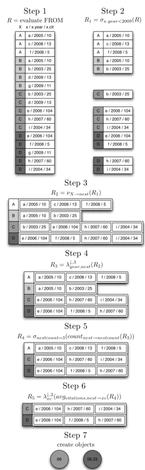
Summarizing the execution strategy of BiQL, we can dis-tinguish several steps. These steps are shown schematically in Figure 5 for the following query, when executed on exam-ple data in Figure 4:
SELECT <X> { color: X.color,
label: avg<x>(x.citations) } FROM author X -> author_of -> publication x WHERE x.year < 2009 AND count<x> = 3 LIMIT LOCAL 3 ON x.year DESC
LIMIT GLOBAL 2 ON avg<x>(x.citations) DESC
This query returns the two authors that have the highest average number of citations on their three most recent pa-pers before 2009. Authors with less than 3 papa-pers in this period are not taken into account. The steps to execute this query are the following, where we also illustrate the use of our algebra:
1. Evaluate the path expressions described in the FROM
statement. This step generates a set of tuples, where each tuple corresponds to a valid assignment to the variables defined in the FROM statement. Alternative strategies can be applied to evaluate these path expres-sions based on their internal structure and the presence of named variables. This is shown in step 1 of Figure 5, where the set of tuples contains all pairs of an author
X and a publicationxthat are connected by an ‘au-thor of’ edge in the network. Only named variables are part of the tuple (so the author-of connection is not present). We call this set of tuplesR.
A B C D a 2005 10 cit. b 2003 25 cit. c 2008 13 cit. d 2009 13 cit. e 2006 104 cit. f 2008 5 cit. g 2009 11 cit. h 2007 60 cit. i 2004 34 cit.
Figure 4: Database graph containing authors (boxes) and publications (circles) connected through an ‘author of’ ob-ject (arrow). Publications contain year of publication and number of citations.
2. Filter the set of tuples based on attribute-based con-straints defined in the WHEREstatement. It should be possible to evaluate each constraint for each tuple indi-vidually. For the example, this corresponds to remov-ing all tuples containremov-ing publication dor g, as shown in step 2 of Figure 5. In algebra, this corresponds to
R1=σx.year<2009(R)
3. Apply nesting to the remaining tuples based on the grouping variables given in the SELECTstatement. In Figure 5 this is done by, for each author, combining all publications into a nested tuple. In algebra, this corresponds to
R2=νX→nest(R1),
where a new element with namenestis introduced. 4. Order and select the top-k tuples based on the
con-ditions given in the (local) LIMIT statement for each tuple-set. For the example, this corresponds to re-moving the oldest publication from the nested tuples corresponding to C and D. The tuples forA and B
remain unchanged, since they already contain three or less items. In algebra, we apply a local limit on the year attribute on the nested tuples:
R3=λ
↓,3
year,nest(R2)
5. Filter the new tuple set based on aggregate-based con-straints defined in the WHERE statement. As before, it should be possible to evaluate each constraint for each tuple individually. In the example, authors with less (or more) than three remaining publications are removed. Step 5 in Figure 5 shows the removal of author B because of this. Note that this step is per-formedafter the local limit statement so tuplesCand
D also satisfy this constraint. In algebra we add an
A A A B B a / 2005 / 10 c / 2008 / 13 f / 2008 / 5 a / 2005 / 10 b / 2003 / 25 C C C C D D D D b / 2003 / 25 e / 2006 / 104 h / 2007 / 60 i / 2004 / 34 e / 2006 / 104 f / 2008 / 5 h / 2007 / 60 i / 2004 / 34 R1=σx.year<2009(R)
Step 2
A A A B B B C C C C C D D D a / 2005 / 10 c / 2008 / 13 f / 2008 / 5 a / 2005 / 10 b / 2003 / 25 D D d / 2009 / 13 b / 2003 / 25 d / 2009 / 13 e / 2006 / 104 h / 2007 / 60 i / 2004 / 34 e / 2006 / 104 f / 2008 / 5 g / 2009 / 11 h / 2007 / 60 i / 2004 / 34 B g / 2009 / 11 X x / x.year / x.cit R= evaluate FROMStep 1
A a / 2005 / 10 c / 2008 / 13 f / 2008 / 5 B a / 2005 / 10 b / 2003 / 25 C b / 2003 / 25 e / 2006 / 104 h / 2007 / 60 i / 2004 / 34 D e / 2006 / 104 f / 2008 / 5 h / 2007 / 60 i / 2004 / 34 R2=νX→nest(R1)
Step 3
A a / 2005 / 10 c / 2008 / 13 f / 2008 / 5 B a / 2005 / 10 b / 2003 / 25 C e / 2006 / 104 h / 2007 / 60 i / 2004 / 34 D e / 2006 / 104 f / 2008 / 5 h / 2007 / 60 R3=λ↓year,nest,3 (R2)Step 4
A a / 2005 / 10 c / 2008 / 13 f / 2008 / 5 C e / 2006 / 104 h / 2007 / 60 i / 2004 / 34 D e / 2006 / 104 f / 2008 / 5 h / 2007 / 60 R4=σnestcount=3(countnest→nestcount(R3))Step 5
C e / 2006 / 104 h / 2007 / 60 i / 2004 / 34 D e / 2006 / 104 f / 2008 / 5 h / 2007 / 60 R5=λ↓xc,2(avgcitations,nest→xc(R4))Step 6
56.33 66create objects
Step 7
rank name #co-authors
1 Muggleton, S. 36
2 Dzeroski, S. 28
3 Blockeel, H. 22
Table 2: Results for query Q1
attribute to represent the aggregate and select on this new attribute:
R4=σnestcount=3(countnest→nestcount(R3))
6. Order and select the top-k tuples based on the con-ditions in the (global) LIMITstatement. In step 6 of Figure 5, the tuple corresponding to author A is re-moved because it has the lowest average number of citations of the three remaining tuples. In algebra we add another attribute for nested tuples and and rank on these attributes:
R5=λ↓xc,2(avgcitations,nest→xc(R4))
7. Create a new object for each of the remaining tuples by generating the attributes and links described in the SELECT statement. As a final result, the exam-ple query generates two new objects corresponding to the remaining tuplesC andD.
6.
EXPERIMENTS
In this section we showcase some of the capabilities of BiQL on the ILPnet2 publication database. A prototype of BiQL was implemented using YAP Prolog. In this im-plementation BiQL queries are essentially transformed into Prolog queries; we exploit the fact that YAP Prolog already has support for BDDs to execute ProbLog-like queries.
In the following we only use three domains from this data-base: author(A),author_of(AO), and,publication(P). First, we add theco-author relation to the network as a connection between authors that have more than one publi-cation in common.
CREATE co-author AS
SELECT <a,b> { a->, b<-, strength: count<p> } FROM A a -> AO -> P p <- AO <- A b
WHERE count<p> > 1
Using this relation we can request the top 3 authors with the most co-authors (Q1).
SELECT a FROM author a -> co-author co LIMIT GLOBAL 3 BY count<co> DESC
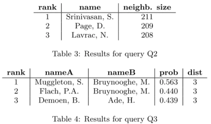
We can also be interested in finding the authors with the largest network of co-authors up to a certain distance (Q2).
SELECT a { network_size: count<b> }
FROM A a -> CA ca -> (A -> CA ca ->)* -> A b WHERE length(ca) < 4
LIMIT GLOBAL 3 BY count<b> DESC
Another interesting task is calculating network analysis metrics such as centrality measures. The easiest centrality measure is degree centrality which can be calculated using BiQL as follows.
EXEC SELECT a { Cdegree: count<ca>/(count<n> - 1)} FROM A a -- CA ca, A n
rank name neighb. size
1 Srinivasan, S. 211
2 Page, D. 209
3 Lavrac, N. 208
Table 3: Results for query Q2
rank nameA nameB prob dist
1 Muggleton, S. Bruynooghe, M. 0.563 3
2 Flach, P.A. Bruynooghe, M. 0.440 3
3 Demoen, B. Ade, H. 0.439 3
Table 4: Results for query Q3
Another common centrality measure is closeness centrality which involves determining the length of the shortest path to all other nodes in the network. First let us define the notion of shortest path between two nodes.
DEFINE ShortestPath AS
SELECT <a,b>{ a->, b<-, len: min<ca>(length(ca))} FROM A a -> CA ca -> (A -> CA ca ->)* -> A b WHERE a != b
LIMIT LOCAL 1 BY length(ca) ASC
Using this new domain, we can easily calculate the closeness centrality as follows.
EXEC SELECT a { Cclose: 1/sum<b>(min<sp>(sp.len))} FROM A a -> ShortestPath sp -> A b
Another important aspect of BiQL is its ability of dealing with probabilistic networks. To illustrate this, we first need to introduce probabilities in our network. For this we as-sume that the information in the network is very unreliable by stating that for each publication in the network there is only 10% probability that it actually exists. Under this assumption we can attach a probability to each co-author connection using the following query.
EXEC SELECT ca { prob: 1-(0.9^ca.strength) } FROM co-author ca
We can now calculate for each pair of authors the probability that they are connected using the probabilistic aggregate
problog_connect.
DEFINE ProbConnect AS SELECT <a,b>{ a->, b<-,
prob: problog_connect(ca.prob) } FROM A a -> CA ca -> (A -> CA ca ->)* -> A b WHERE a != b
As a final step we can use this domain in combination with the shortest path to find authors that are very likely con-nected, but that are relatively far apart in the co-author network (Q3).
SELECT <a,b,pc,sp>
{nameA: a.name, nameB: b.name,
prob: pc.prob, dist: sp.length } FROM A a -> ProbConnect pc -> A b,
#a -> ShortestPath sp -> #b WHERE sp.length > 2
LIMIT GLOBAL 1 BY pc.prob DESC
7.
CONCLUSIONS
Motivated by the need to have database support for the analysis and mining of large networks we proposed several
extensions to a previously proposed data model and query language (BiQL). The main elements of these extensions were aggregates, rankings and path expressions; they al-lowed us to calculate well-known network statistics (such as centrality measures), transform networks for the application of more advanced mining algorithms or more complex prob-abilistic measures (such as connection probabilities). We implemented our language in a Prolog-based prototype.
The main challenge we are currently facing is the develop-ment of a more scalable impledevelop-mentation. To a certain degree our approach seems incompatible with recent work on large-scale storage systems (such as the Hadoop File System or Google’s BigTable). Our language supports operations such as subgraph isomorphism, which are known to be NP hard to compute; hence it is not likely that our language (or any other language supporting this operation) will scale to the datasets of billions of nodes that the HFS and BigTable are required for. Still, we believe there is a need for expressive query languages for smaller datasets. On such datasets, sev-eral common queries, such as shortest path queries, may be optimized by running specialized algorithms. A theoretical framework for the evaluation of queries with such optimiza-tions is currently missing, even though some more simple optimizations are not too hard to obtain: for instance, when a query is posed in which path expressions are used without variables that collect the objects in the path, we can deduce that finding one path satisfying the regular expression is suf-ficient; in such case we can avoid considering a potentially exponential number of paths between nodes, and can per-form a dynamic programming style of algorithm. This may still not be feasible on very large graphs, but already scales much better to datasets of thousands of nodes.
Further optimizations may be obtained by more carefully considering how graphs are stored. Our current implemen-tation relies on an in-memory Prolog or on-disk relational database. The first option is reasonably fast, but is not per-sistent; the latter option is persistent but not efficient. By implementing our language on top of a graph database, such as Neo4J [18] or Dex [16], our language could become more widely applicable.
A possible use of our query language is in systems for Inductive Logic Programming. In many such systems a hy-pothesis language needs to be defined through which the system searches; a BiQL query may serve as a hypothesis.
Finally, we aim to study several open questions concern-ing the formulation of graph queries. In recent work [21] a higher-level programming language called Gremlin was de-veloped for implementing PageRank-like measures on net-works. This language however does not support the more declarative querying that we are proponents of. Extending our language with primitives for expressing measures such as PageRank may increase the flexibility of our language.
Acknowledgements.
This work was supported by the Euro-pean Commission under the 7th Framework Programme FP7-ICT-2007-C FET-Open, contract no. BISON-211898 and by a Postdoc grant from the Research Foundation — Flanders.8.
REFERENCES
[1] B. Amann and M. Scholl. Gram: a graph data model and query language. InHT, pages 201–211. 1992. [2] R. Angles and C. Gutierrez. Survey of graph database
models.ACM Computing Surveys, 40(1):1–39, 2008.
[3] I. Bhattacharya and L. Getoor. Collective entity resolution in relational data.Data Engineering Bulletin, 29(2):4–12, 2006.
[4] S. Brin and L. Page. The anatomy of a large-scale hypertextual web search engine.Computer Networks, 30(1-7):107–117, 1998.
[5] L. De Raedt, A. Kimmig, H. Toivonen. ProbLog: A Probabilistic Prolog and Its Application in Link Discovery. InIJCAI, pages 2462–2467, 2007. [6] A. Dries, S. Nijssen and L. De Raedt. A query
language for analyzing networks. InCIKM, pages 485–494, 2009.
[7] R. H. G¨uting. GraphDB: Modeling and querying graphs in databases. InVLDB, pages 297–308, 1994. [8] M. Gyssens, J. Paredaens, and D. van Gucht. A
graph-oriented object database model. InPODS, pages 417–424. ACM, 1990.
[9] J. Han, and M. Kamber.Data Mining: Concepts and Techniques. 2nd edition, Morgan Kaufmann, 2006. [10] H. He and A. K. Singh. Graphs-at-a-time: query
language and access methods for graph databases. In
SIGMOD, pages 405–418. ACM, 2008.
[11] J. Hidders. Typing graph manipulation operations. In
ICDT, pages 394–409. Springer-Verlag, 2003. [12] G. Karypis and V. Kumar. Multilevel k-way
partitioning scheme for irregular graphs.J. on Parallel and Distributed Computing, 48(1):96–129, 1998. [13] U. Leser. A query language for biological networks.
Bioinformatics, 21(2):33–39, 2005.
[14] M. Levene and A. Poulovassilis. The hypernode model and its associated query language. InJCIT, pages 520–530. IEEE Computer Society Press, 1990. [15] M. Levene and A. Poulovassilis. An object-oriented
data model formalised through hypergraphs.Data and Knowledge Engineering, 6(3):205–224, 1991.
[16] N. Mart´ınez-Bazan, V. Munt´es-Mulero, S.
G´omez-Villamor, J. Nin, M. S´anchez-Mart´ınez and J. Larriba-Pey Dex: high-performance exploration on large graphs for information retrieval. InCIKM, pages 573–582, 2007.
[17] The iGraph library.
http://igraph.sourceforge.net/. [18] The Neo4J Project.http://neo4j.org/. [19] Jure Leskovec. SNAP Library.
http://snap.stanford.edu/snap/.
[20] E. Prud’hommeaux and A. Seaborne. SPARQL query language for RDF.
http://www.w3.org/TR/rdf-sparql-query/. [21] Marko A. Rodriguez.
http://wiki.github.com/tinkerpop/gremlin/. [22] P. Sen, G. Namata, M. Bilgic, L. Getoor, B. Gallagher,
and T. Eliassi-Rad. Collective classification in network data.AI Magazine, 29(3):93–107, 2008.
[23] L. Sheng, Z. Ozsoyoglu, and G. Ozsoyogly. A graph query language and its query processing. InICDE, pages 572–581. IEEE Computer Society Press, 1999. [24] J. Wicker, L. Richter, K. Kessler, and S. Kramer.
SINDBAD and SiQL: An inductive database and query language in the relational model. In