September 2015
Multiple Testing for Neuroimaging via Hidden Markov Random Field
Hai Shu,1 Bin Nan,1,*and Robert Koeppe21Department of Biostatistics, University of Michigan, Ann Arbor, Michigan 48109, U.S.A.
2Department of Radiology, University of Michigan, Ann Arbor, Michigan 48109, U.S.A.
∗email:[email protected]
Summary. Traditional voxel-level multiple testing procedures in neuroimaging, mostlyp-value based, often ignore the spatial correlations among neighboring voxels and thus suffer from substantial loss of power. We extend the local-significance-index based procedure originally developed for the hidden Markov chain models, which aims to minimize the false nondiscovery rate subject to a constraint on the false discovery rate, to three-dimensional neuroimaging data using a hidden Markov random field model. A generalized expectation–maximization algorithm for maximizing the penalized likelihood is proposed for estimating the model parameters. Extensive simulations show that the proposed approach is more powerful than conventional false discovery rate procedures. We apply the method to the comparison between mild cognitive impairment, a disease status with increased risk of developing Alzheimer’s or another dementia, and normal controls in the FDG-PET imaging study of the Alzheimer’s Disease Neuroimaging Initiative.
Key words: Alzheimer’s disease; False discovery rate; Generalized expectation–maximization algorithm; Ising model; Local significance index; Penalized likelihood.
1. Introduction
In a seminal article, Benjamini and Hochberg (1995) intro-duced false discovery rate (FDR) as an alternative measure of Type I error in multiple testing problems to the family-wise error rate (FWER). They showed that the FDR is equiv-alent to the FWER if all null hypotheses are true and is smaller otherwise, thus FDR controlling procedures poten-tially have a gain in power over FWER controlling procedures. FDR is defined as the expected proportion of false rejec-tions among all rejecrejec-tions. The false nondiscovery rate (FNR; Genovese and Wasserman, 2002), the expected proportion of falsely accepted hypotheses, is the corresponding measure of Type II error. The traditional FDR procedures (Benjamini and Hochberg, 1995, 2000; Genovese and Wasserman, 2004), which arep-value based, are theoretically developed under the assumption that the test statistics are independent. Although these approaches are shown to be valid in controlling FDR under certain dependence assumptions (Benjamini and Yeku-tieli, 2001; Farcomeni, 2007; Wu, 2008), they may suffer from severe loss of power when the dependence structure is ignored (Sun and Cai, 2009). By modeling the dependence structure using a hidden Markov chain (HMC), Sun and Cai (2009) pro-posed an oracle FDR procedure built on a new test statistic, the local index of significance (LIS), and the corresponding asymptotic data-driven procedure, which are optimal in the sense that they minimize the marginal FNR subject to a con-straint on the marginal FDR. Following the work of Sun and Cai (2009), Wei et al. (2009) developed a pooled LIS (PLIS) procedure for multiple-group analysis where different groups have different HMC dependence structures, and proved the optimality of the PLIS procedure. Either the LIS procedure
or the PLIS procedure only handles the one-dimensional de-pendency. However, problems with higher dimensional depen-dence are of particular practical interest in analyzing imaging data.
FDR procedures have been widely used in analyzing neu-roimaging data, such as positron emission tomography (PET) imaging and functional magnetic resonance imaging (fMRI) data (Genovese, Lazar, and Nichols, 2002; Chumbley and Fris-ton, 2009; Chumbley et al., 2010, among many others). We extend the work of Sun and Cai (2009) in this article by developing an optimal LIS-based FDR procedure for three-dimensional (3D) imaging data using a hidden Markov ran-dom field model (HMRF) for the spatial dependency among multiple tests. Existing methods for correlated imaging data, for example, Zhang, Fan, and Yu (2011) are not shown to be optimal, i.e., minimizing FNR.
HMRF model is a generalization of HMC model, which re-places the underlying Markov chain by Markov random field. A well-known classical Markov random field with two states is the Ising model. In particular, the two-parameter Ising model, whose formal definition is given in equation (1), reduces to the two-state Markov chain in one-dimension (Bremaud, 1999). The Ising model and its generalization with more than two states, the Potts model, have been widely used to capture the spatial structure in image analysis; see Bremaud (1999), Winkler (2003), Zhang et al. (2008), Huang et al. (2013) and Johnson et al. (2013), among others. In this article, we con-sider a hidden Ising model for each area based on the Brod-mann’s partition of the cerebral cortex (Garey, 2006) and subcortical regions of the human brain, which provides a nat-ural way of modeling spatial correlations for neuroimaging
data. To the best of our knowledge, this is the first work that introduces the HMRF-LIS based FDR procedure to the field of neuroimaging.
We propose a generalized expectation-maximization algo-rithm (GEM; Dempster et al., 1977) to search for penalized maximum likelihood estimators (Ridolfi, 1997; Ciuperca, Ri-dolfi, and Idier, 2003; Chen, Tan, and Zhang, 2008) of the hidden Ising model parameters. The penalized likelihood pre-vents the unboundedness of the likelihood function, and the proposed GEM uses Monte Carlo averages via Gibbs sampler (Geman and Geman, 1984; Roberts and Smith, 1994) to over-come the intractability of computing the normalizing constant in the underlying Ising model. Then the LIS-based FDR pro-cedures can be conducted by plugging in the estimates of the hidden Ising model parameters. In what follows, we use the term “HMRF” to refer to the 3D hidden Ising model.
The article is organized as follows. In Section 2, we intro-duce the HMRF model, i.e., the hidden Ising model, for 3D imaging data. We provide the GEM algorithm for the HMRF parameter estimation and the implementation of the HMRF-LIS-based data-driven procedures in Section 3. In Section 4, we conduct extensive simulations to compare the LIS-based procedures with conventional FDR methods. In Section 5, we apply the PLIS procedure to the 18F-Fluorodeoxyglucose PET (FDG-PET) image data of the Alzheimer’s Disease Neu-roimaging Initiative (ADNI), which finds more signals than conventional methods.
2. A Hidden Markov Random Field Model
LetS be a finite lattice ofN voxels in an image grid, usually in a 3D space. Let= {s∈ {0,1}:s∈S}denote the set of latent states onS, wheres=1 if the null hypothesis at voxel
s is false ands=0 otherwise. For simplicity, we follow Sun and Cai (2009) to call hypothesissto be nonnull ifs=1 and null otherwise. We also call voxelsto be a signal ifs=1 and noise otherwise. Let be generated from a two-parameter Ising model with the following probability distribution
Pϕ(θ)= 1 Z(ϕ)exp{ϕ TH(θ)} = 1 Z(β, h)exp β s,t θsθt+h s∈S θs , (1)
where Z(ϕ) is the normalizing constant, ϕ=(β, h)T,H(θ)= (s,tθsθt,
s∈Sθs)
T, ands, tdenotes all the unordered pairs inS such that for anys,tis among the six nearest neighbors of voxel sin a 3D setting. This model possesses the Markov property: Pϕ(θs|θS\{s})=Pϕ(θs|θN(s)) = exp{θs(β t∈N(s)θt+h)} 1+exp{βt∈N(s)θt+h} ,
whereS\ {s}denotes the setSafter removings, andN(s)⊂S is the nearest neighborhood ofsinS. Some parameter inter-pretations ofβandhare given in Web Appendix A.
We assume the observedz-valuesX= {Xs:s∈S}are inde-pendent given=θwith
Pφ(x|θ)= s∈S
Pφ(xs|θs), (2) wherePφ(xs|θs) denotes the following distribution
Xs|s∼(1−s)N(μ0, σ20)+s L l=1 plN(μl, σl2) (3) with (μ0, σ2 0)=(0,1), unknown parameters φ=(μ1, σ12, p1, . . ., μL, σL2, pL)T, L
l=1pl=1 andpl≥0. In particular, the
z-value Xs follows the standard normal distribution under the null, and the nonnull distribution is set to be the nor-mal mixture that can be used to approximate a large collec-tion of distribucollec-tions (Magder and Zeger, 1996; Efron, 2004). The number of componentsLin the nonnull distribution may be selected by, for example, the Akaike or Bayesian informa-tion criterion. Following the recommendainforma-tion of Sun and Cai (2009), we useL=2 for the ADNI image analysis.
Markov random fields (MRFs; Bremaud, 1999) are a natu-ral genenatu-ralization of Markov chains (MCs), where the time index of MC is replaced by the space index of MRF. It is well known that any one-dimensional MC is an MRF, and any one-dimensional stationary finite-valued MRF is an MC (Chandgotia et al., 2014). When S is taken to be one-dimensional, the above approach based on (1)–(3) reduces to the HMC method of Sun and Cai (2009).
3. Hidden Markov Random Field LIS-Based FDR Procedures
Sun and Cai (2009) developed a compound decision theoretic framework for multiple testing under HMC dependence and proposed LIS-based oracle and data-driven testing procedures that aim to minimize the FNR subject to a constraint on FDR. We extend these procedures under HMRF for image data. The oracle LIS for hypothesissis defined asLISs(x)=
P(s=0|x) for a given parameter vector. In our model, =(φT
,ϕT)T. LetLIS(1)(x), . . ., LIS(
N)(x) be the ordered LIS values andH(1), . . .,H(N) the corresponding null hypotheses. The oracle procedure operates as follows: for a prespecified FDR levelα, letk=max i:1 i i j=1 LIS(j)(x)≤α ,
then reject allH(i), i=1, . . ., k. (4) Parameter is unknown in practice. We can use the data-driven procedure that simply replaces LIS(i)(x) in (4) with
LIS(i)(x)=Pˆ((i)=0|x), where ˆis an estimate of. If all the tests are partitioned into multiple groups and each group follows its own HMRF, in contrast to the separated LIS (SLIS) procedure that conducts the LIS-based FDR procedure separately for each group at the same FDR levelαand then combines the testing results, we follow Wei et al. (2009) to propose a pooled LIS (PLIS) procedure that is more efficient
in reducing the global FNR. The PLIS follows the same pro-cedure as (4), but with LIS(1), . . ., LIS(N) being the ordered test statistics from all groups.
Note that the model homogeneity, which is required in Sun and Cai (2009) and Wei et al. (2009) for HMCs, fails to hold for the HMRF model. In other words,P(s=1) for the interior voxels with six nearest neighbors are different to those for the boundary voxels with less than six nearest neighbors. We show the validity and optimality of the oracle HMRF-LIS-based procedures in Web Appendix B.
We now provide details of the LIS-based data-driven proce-dure for 3D image data, where the parameters of the HMRF model need to be estimated from observed test data. 3.1. A Generalized EM Algorithm
The observed likelihood function under HMRF, L(|x)= P(x)=Pφ(x|)Pϕ(), is unbounded (see Web Ap-pendix C for details). One solution to avoid the unbound-edness is to replace the likelihood by a penalized likeli-hood (Ridolfi, 1997; Ciuperca et al., 2003)
pL(|x)=L(|x) L l=1 g(σl2), (5) where g(σ2
l), l=1, . . . , L, are penalty functions that ensure the boundedness of pL(|x). We follow Ridolfi (1997) and Ciuperca et al. (2003) to choose
g(σ2 l)∝ 1 σ2b l exp − a σ2 l , a >0, b≥0,
wherex∝ymeans thatx=cywith a positive constantc in-dependent of any parameter. Note that (5) reduces to the unpenalized likelihood function whena=b=0. Whena >0 andb >1, the penalized likelihood approach is equivalent to settingg(σ2
l) to be the inverse gamma distribution, which is a classical prior distribution for the variance of a normal distri-bution in Bayesian statistics (Hoff, 2009). We do not impose any prior distribution here. The choice ofa and bdoes not impact the strong consistency of the penalized maximum like-lihood estimator (PMLE) based on the same penalty function for a finite mixture of normal distributions (Ciuperca et al., 2003; Chen et al., 2008). Such a penalty performs well in the simulations, though formal proof of the consistency of PMLE for hidden Ising model remains an open question.
We develop an EM algorithm based on the penalized likeli-hood (5) for the estimation of parameters in the HMRF model characterized by (1)–(3). We introduce unobservable categori cal variablesK= {Ks:s∈S}, whereKs=0 ifs=0, andKs∈
{1, . . ., L}ifs=1. Hence,P(Ks=0|s=0)=1 and we denote
P(Ks=l|s=1)=pl. From (3), we letXs|Ks∼N(μKs, σ 2
Ks). To estimate the HMRF parameters=(φT,ϕT)T, (,K,X) are used as the complete data variables to construct the auxiliary function in the (t+1)st iteration of EM algorithm given the observed dataxand the current estimated parameters(t):
Q(|(t) )=E(t)[logP(,K,X)|x]+ L l=1 logg(σl2), whereP(,K,X)=Pϕ()Pφ(X,K|)=Pϕ()s∈SPφ(Xs,
Ks|s). TheQ-function can be further written as follows
Q(|(t))=Q1(φ|(t))+Q2(ϕ|(t)), where Q1(φ|(t))= K P(t)(,K|x) logPφ(x,K|) + L l=1 logg(σl2) and Q2(ϕ|(t))= P(t)(|x) logPϕ().
Therefore, we can maximizeQ(|(t)) forby maximizing Q1(φ|(t)
) forφandQ2(ϕ|(t)
) forϕ, separately.
MaximizingQ1(φ|(t)) under the constraintLl=1pl=1 by the method of Lagrange multipliers yields,
p(lt+1)= s∈Sw (t) s (l) s∈Sγ (t) s (1) , (6) μ(lt+1)= s∈Sw (t) s (l)xs s∈Sw (t) s (l) , (7) (σ2 l) (t+1)= 2a+ s∈Sw (t) s (l)(xs−μ (t+1) l ) 2 2b+s∈Sw(st)(l) , (8) where ws(l)= γs(1)plfl(xs) f(xs) , γs(i)=P(s=i|x), fl =N(μl, σl2), andf = L l=1 plfl.
For Q2(ϕ|(t)), taking its first and second derivatives with respect toϕ, we obtain U(t+1)(ϕ)= ∂ ∂ϕQ2(ϕ| (t)) =E(t)[H()|x]−Eϕ[H()], I(ϕ)= − ∂ 2 ∂ϕ∂ϕTQ2(ϕ| (t))=Varϕ[H()]. MaximizingQ2(ϕ|(t)) is then equivalent to solving the non-linear equation:
U(t+1)
It can be shown that equation (9) has a unique solution and can be solved by the Newton-Raphson (NR) method (Stoer and Bulirsch, 2002). However, a starting point that is not close enough to the solution may result in divergence of the NR method. Therefore, rather than searching for the solution of equation (9) over all ϕ, we choose aϕ(t+1) that increases Q2(ϕ|(t)) over its value atϕ=ϕ(t). Together with the maxi-mization ofQ1(φ|(t)
), the approach leads toQ((t+1)|
(t) )≥ Q((t)|(t)) and thus pL((t+1)|x)≥pL((t)|x), which is termed a GEM algorithm (Dempster, Laird, and Rubin, 1977). To find such a ϕ(t+1) that increases the Q2-function, a backtracking line search algorithm (Nocedal and Wright, 2006) is applied with a set of decreasing positive valuesλm in the following
ϕ(t+1,m)=ϕ(t)+λ
mI(ϕ(t))−1U(t+1)(ϕ(t)), (10)
wherem=0,1, . . .,andϕ(t+1)=ϕ(t+1,m)which is the first one satisfying the Armijo condition (Nocedal and Wright, 2006)
Q2(ϕ(t+1,m)| (t) )−Q2(ϕ(t)| (t) ) ≥αλmU(t+1)(ϕ(t))TI(ϕ(t))−1U(t+1)(ϕ(t)). (11) Since I(ϕ(t)) is positive-definite, the Armijo condition guar-antees the increase ofQ2-function. In practice,αis chosen to be quite small. We adoptα=10−4, which is recommended by Nocedal and Wright (2006), and halve the Newton–Raphson step length each time by usingλm=2−m.
In the GEM algorithm, Monte Carlo averages are used via Gibbs sampler to approximate the quantities of interest that are involved with the intractable normalizing constant of the Ising model. By the ergodic theorem of the Gibbs sampler (Roberts and Smith, 1994) (see Web Appendix D for details),
U(t+1) (ϕ)≈ 1 n n i=1 H(θ(t,i,x) )−H(θ(i,ϕ) ), I(ϕ)≈ 1 n−1 n i=1 H(θ(i,ϕ) )−1 n n j=1 H(θ(j,ϕ) ) ⊗2 , where{θ(t,1,x) , . . .,θ(t,n,x)}are large
nsamples successively gen-erated by the Gibbs sampler from
P(t)(θ|x)= exp β(t) s,rθsθr+ s∈Sh (t) s θs Z β(t),{h(t) s }s∈S , with h(st)=h(t)−log 1 2πσ2 0 exp −(xs−μ0)2 2σ2 0 +log ⎛ ⎝L l=1 p(lt) 2πσ2(t) l exp −(xs−μ (t) l ) 2 2σ2(t) l ⎞ ⎠ and Z β(t),{h(t) s }s∈S
being the normalizing constant, and
{θ(1,ϕ), ...,θ(n,ϕ)}are generated fromPϕ(θ). Here for vectorv, v⊗2=vvT. Similarly, C Z(ϕ) =Eϕ[exp{−ϕ T H()}]≈ 1 n n i=1 exp{−ϕTH(θ(i,ϕ))}, where Cis the number of all possible configurations θ of. Then the difference betweenQ2-functions in the Armijo con-dition can be approximated by
Q2(ϕ(t+1,m)|(t))−Q2(ϕ(t)|(t)) ≈ 1 n(ϕ (t+1,m)−ϕ(t))T n i=1 H(θ(t,i,x)) +log n i=1exp{−ϕ (t+1,m)TH(θ(i,ϕ(t+1,m)) )} n i=1exp{−ϕ (t)TH(θ(i,ϕ(t)) )} .
Back to Q1(φ|(t)), the local conditional probability of givenxcan also be approximated by the Gibbs sampler:
γ(t) s (i)=P(t)(s=i|x)≈ 1 n n k=1 1(θ(t,k,x) s =i). (12)
3.2. Implementation of the LIS-Based FDR Procedure The algorithm for the LIS-based data-driven procedure, de-noted as LIS for single group analysis, SLIS for separate anal-ysis of multiple groups, and PLIS for pooled analanal-ysis for mul-tiple groups, is given below:
1. Set initial values(0)= {φ(0)
,ϕ(0)}for the model param-etersof each group;
2. Updateφ(t)from equations (6), (7) and (8); 3. Updateϕ(t)from equations (10) and (11);
4. Iterate Steps 2 and 3 until convergence, then obtain the estimate ˆof;
5. Plug-in ˆto obtain the test statisticsLISfrom equation (12);
6. Apply the data-driven procedure (LIS, SLIS, or PLIS). The GEM algorithm is stopped when the following stopping rule max i |(it+1)− (t) i | |(it)| +1 < 2, (13)
where i is the ith coordinate of vector , is satisfied for three consecutive regular Newton–Raphson iterations with m=0 in (10), or the prespecified maximum number of it-erations is reached. Stopping rule (13) was applied by Booth and Hobert (1999) to the Monte Carlo EM method, where they set1=0.001,2 between 0.002 and 0.005, and the rule to be satisfied for three consecutive iterations to avoid stop-ping the algorithm prematurely because of Monte Carlo error.
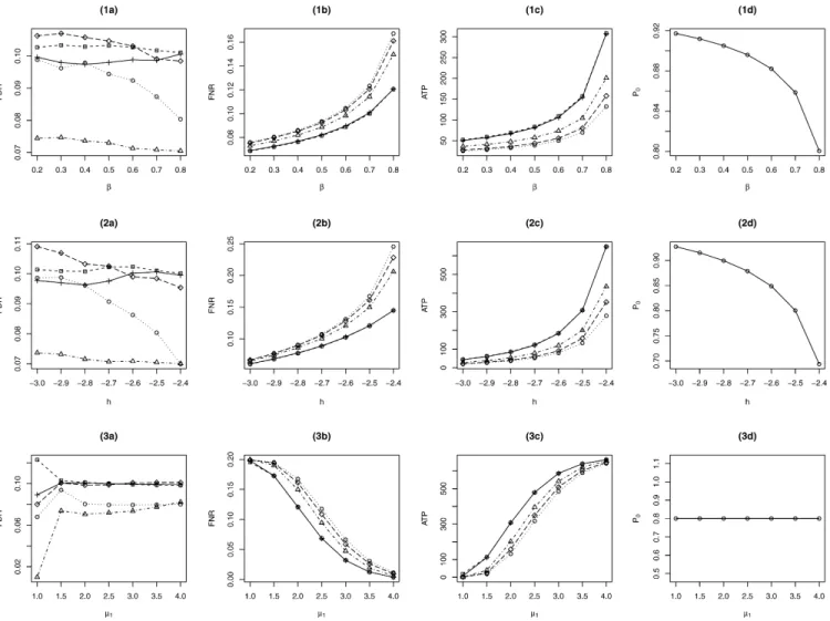
Figure 1. Comparison of BH (),q-value (), Lfdr (), OR (+), and LIS () for a single group withL=1. We used1=2=0.001 in simulation studies and real-data
analysis. Constantα=10−4 is recommended by Nocedal and Wright (2006) for the Armijo condition (11), and the Newton– Raphson step length in (10) is halved by using λm=2−m . In practice, the Armijo condition (11) might not be satisfied when the step length ϕ(t+1,m)−ϕ(t) is very small. In this situation, the iteration within Step 3 is stopped by an alter-native criterion max i |ϕ(it+1,m)−ϕ (t) i | |ϕ(it)| +1 < 3
with3< 2, for example,3=10−4if2=0.001. Smallaand bshould be chosen in (8). We choosea=1 andb=2.
4. Simulation Studies
The simulation setups are similar to those in Sun and Cai (2009) and Wei et al. (2009), but with 3D data. The performances of the proposed LIS-based oracle (OR) and data-driven procedures are compared with the BH approach
(Benjamini and Hochberg, 1995), the q-value procedure (Storey, 2003), and the local FDR (Lfdr) procedure (Sun and Cai, 2007) for single group analysis; and the performances of SLIS and PLIS are compared with BH, q-value, and the conditional Lfdr (CLfdr) procedure (Cai and Sun, 2009) for multiple groups. The Lfdr and CLfdr procedures are shown to be optimal for independent tests (Sun and Cai, 2007; Cai and Sun, 2009). For simulations with multiple groups, all the procedures are globally implemented using all the lo-cally computed test statistics based on each method from each group. The q-values are obtained using the R package qvalue (Dabney and Storey, 2014). For the Lfdr or CLfdr procedure, we use the proportion of the null cases generated from the Ising model with given parameters as the estimate of the probability of the null casesP(s=0), together with the given null and nonnull distributions without estimating their parameters. For the LIS-based data-driven procedures, the maximum number of GEM iterations is set to be 1000 with1=2=0.001,3=α=10−4,a=1 andb=2. For the Gibbs sampler, 5000 samples are generated from 5000 itera-tions after a burn-in period of 1000 iteraitera-tions. In all simula-tions, each HMRF is on aN=15×15×15 cubic latticeS, the
Figure 2. Comparison of BH (),q-value (), Lfdr (), OR (+), and LIS () for a single group withL=2 (see 1a–2c), and the one withLbeing misspecified (see 3a–c).
number of replications M=200 is the same as that in Wei et al. (2009), and the nominal FDR level is set at 0.10. 4.1. Single-Group Analysis
4.1.1. Study 1:L=1. The MRF= {s:s∈S}is gen-erated from the Ising model (1) with parameters (β, h), and the observationsX= {Xs:s∈S}are generated conditionally onfromXs|s∼(1−s)N(0,1)+sN(μ1, σ21). Note that the MRF is not observable in practice. Figure 1 shows the comparisons of the performance of BH,q-value, Lfdr, OR and LIS. In Figure 1(1a-1c), we fixh= −2.5, setμ1=2 and σ2
1=1, and plot FDR, FNR, and the average number of true positives (ATP) yielded by these procedures as functions of
β. In Figure 1(2a-2c), we fixβ=0.8, setμ1=2 and σ2 1 =1, and plot FDR, FNR and ATP as functions of h. In Figure 1(3a–c), we fix β=0.8 and h= −2.5, set σ2
1=1, and plot FDR, FNR and ATP as functions of μ1. The corresponding average proportions of the nulls, denoted byP0, for each Ising model are given in Figure 1(1d–3d). The initial values for the numerical algorithm are set atβ(0)=h(0)=0, μ(0)
1 =μ1+1 andσ12(0)=2.
From Figure 1(1a–3a), we can see that the FDR levels of all five procedures are controlled around 0.10 except one case of the LIS procedure in Figure 1(3a) with the lowestμ1, whereas the BH and Lfdr procedures are generally conservative. This case of obvious deviation of the LIS procedure is likely caused
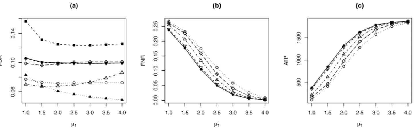
Figure 3. Comparison of BH (), q-value (), CLfdr (), SLIS (), and PLIS (•) for two groups withL=1. In (a), andrepresent the results by PLIS for each individual group; for PLIS, while the global FDR is controlled, individual-group FDRs may vary.
by the small lattice sizeN. As a confirmation, additional sim-ulations by increasing the lattice sizeN to 30×30×30 yield an FDR of 0.1019 for the same setup. From Figure 1(1b– 3b) and (1c–3c) we can see that the two curves of OR and LIS procedures are almost identical, indicating that the data-driven LIS procedure works equally well as the OR procedure. These plots also show that the LIS procedure outperforms BH, q-value and Lfdr procedures with increased margin of performance in FNR and ATP as β or h increases or μ1 is at a moderate level. Note that from Web Appendix A, we can see thatβcontrols how likely the same-state cases clus-ter together, and (β, h) together control the proportion of the aggregation of nonnulls relative to that of nulls.
4.1.2. Study 2: L=2. We now consider the case where the nonnull distribution is a mixture of two normal distribu-tions. The MRF is generated from the Ising model (1) with fixed parametersβ=0.8 and h= −2.5, and the nonnull dis-tribution is a two-component normal mixturep1N(μ1, σ2
1)+ p2N(μ2, σ2
2) with fixedp1=p2=0.5,μ2=2,andσ 2 2=1. In Figure 2(1a–c),σ2
1varies from 0.125 to 8, andμ1= −2. In Fig-ure 2(2a–c), we fixσ2
1 =1 and vary μ1 from −4 to−1. The initial values are set atβ(0)=h(0)=0,p(0)
1 =1−p (0) 2 =0.3, μ(0)l =μl+1,andσ 2(0) l =σl2+1, l=1,2.
Similar to Figure 1, we can see that the FDR levels of all the procedures are controlled around 0.10, where BH and Lfdr are conservative, and OR and LIS perform similarly and outperform the other three procedures. In Figure 2(2a) at μ1= −1, additional simulations yield an FDR of 0.1035 when the lattice sizeNis increased to 30×30×30 for the same setup. The results from both simulation studies are very similar to those in Sun and Cai (2009) for the one-dimensional case us-ing HMC. It is clearly seen that, for dependent tests, incorpo-rating dependence structure into a multiple-testing procedure improves efficiency dramatically.
4.1.3. Study 3: misspecified nonnull. Following Sun and Cai (2009), we consider the true nonnull distribution to be the three-component normal mixture 0.4N(μ,1)+0.3N(1,1)+ 0.3N(3,1), but use a misspecified two component normal mix-ture p1N(μ1, σ2
1)+p2N(μ2, σ22) in the LIS procedure. The
unobservable states are generated from the Ising model (1) with fixed parametersβ=0.8 andh= −2.5. The simulation results are displayed in Figure 2(3a–c), the trueμvaries from
−4 to−1 with increments of size 0.5. The initial values are set at β(0)=h(0)=0,p(0) 1 =p (0) 2 =0.5,μ (0) 1 = −μ (0) 2 = −2, and σl2(0)=2, l=1,2.
Figure 2(3a–c) shows that the LIS procedure performs sim-ilarly to OR under misspecified model. Additionally, the obvi-ous biased FDR level by the LIS procedure atμ= −1 reduces to 0.1067 when the lattice sizeNis increased to 30×30×30. 4.2. Multiple-Group Analysis
Voxels in a human brain can be naturally grouped into multi-ple functional regions. For simulations with grouped multimulti-ple tests, we consider two lattice groups each with size 15×15×15. The corresponding MRFs1= {1s:s∈S}and2= {2s:
s∈S} are generated from the Ising model (1) with param-eters (β1=0.2, h1= −1) and (β2=0.8, h2= −2.5), respec-tively. The observations Xk= {Xks, s∈S} are generated con-ditionally on k,k=1,2, fromXks|ks∼(1−ks)N(0,1)+
ksN(μk, σk2), where μ1 varies from 1 to 4 with increments of size 0.5, μ2=μ1+1 and σ2
1 =σ 2
2 =1. The initial values are β(0)1 =β(0)2 =h(0)1 =h2(0)=0, μ(0)2 =μ(0)1 =μ1+1, and σ2(0)
1 =σ2 (0) 2 =2.
The simulation results are presented in Figure 3, which are similar to that in Wei et al. (2009) for the one-dimensional case with multiple groups using HMCs. Figure 3(a) shows that all procedures are valid in controlling FDR at the pre-specified level of 0.10, whereas BH and CLfdr procedures are conservative. We also plot the within-group FDR levels of PLIS for each group separately. One can see that in order to minimize the global FNR level, the PLIS procedure may automatically adjust the FDRs of each individual group, ei-ther inflated or deflated reflecting the group heterogeneity, while the global FDR is appropriately controlled. In Figure 3(b) and (c) we can see that both SLIS and PLIS outperform BH, q-value and CLfdr procedures, indicating that utilizing the dependency information can improve the efficiency of a testing procedure, and the improvement is more evident for weaker signals (smaller values of μ1). Between the two
LIS-Figure 4. Z-values of the signals found by each procedure for the comparison between NC and MCI. based procedures, PLIS slightly outperforms SLIS, indicating
the benefit of ranking the LIS test statistics globally. In partic-ular, ATP is 8.3% higher for PLIS than for SLIS whenμ1=1.
5. ADNI FDG-PET Image Data Analysis
Alzheimer’s disease (AD) is the most common cause of de-mentia in the elderly population. Much progress has been made in the diagnosis of AD including clinical assessment and neuroimaging techniques. One such extensively used neu-roimaging technique is FDG-PET imaging, which is used to evaluate the cerebral metabolic rate of glucose (CMRgl). We consider the FDG-PET image data from the ADNI database (adni.loni.usc.edu) as an illustrative example.
The data set consists of the baseline FDG-PET images of 102 normal control (NC) subjects and 206 patients with mild cognitive impairment (MCI), a prodromal stage of AD. Sixty one brain regions of interest (ROIs) are considered (see Web Appendix E for details), where the number of voxels in each region ranges from 149 to 20,680 with a median of 2,517. The total number of voxels of these 61 ROIs isN=251,500. The goal is to identify voxels with reduced CMRgl in MCI patients comparing to NC.
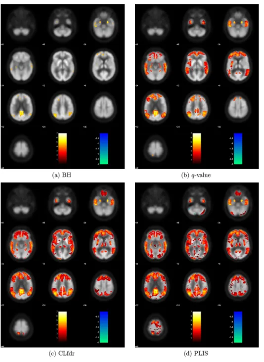
We apply the HMRF-PLIS procedure to the ADNI data, and compare to BH,q-value and CLfdr procedures. We im-plement the BH procedure globally for the 61 ROIs, whereas we treat each region as a group for the q-value, CLfdr and
BH q−value CLfdr PLIS 3 656 9156 33976 0 0 9 1318 460 43780 3 0 48 60116 8478 93497
Figure 5. Venn diagram for the number of signals found by each procedure for the comparison between NC and MCI. Number of signals discovered by each procedure: BH=8,541, q-value=71,031, CLfdr=122,899, and PLIS=146,867. PLIS procedures. For the BH andq-value procedures, a to-tal number ofNtwo-sample Welch’st-tests (Welch, 1947) are performed, and their corresponding two-sidedp-values are ob-tained. For the PLIS and CLfdr procedures,z-values are used as the observed datax, which are obtained from thoset statis-tics by the transformationzi=−1[G0(ti)], whereandG0 are the cumulative distribution functions of the standard nor-mal and thet statistic, respectively. The null distribution is assumed to be the standard normal distribution. The nonnull distribution is assumed to be a two-component normal mix-ture for PLIS. The LIS statistics in the PLIS procedure are approximated by 106 Gibbs-sampler samples, and the Lfdr statistics in the CLfdr procedure are computed by using the R code of Sun and Cai (2007). All the four testing procedures are controlled at a nominal FDR level of 0.001. In the GEM algorithm for HMRF estimation, the initial values forβand h in the Ising model are set to be zero. The initial values for the nonnull distributions are estimated from the signals claimed by BH at an FDR level of 0.1. The maximum num-ber of GEM iterations is set to be 5000 with1=2=0.001, 3=α=10−4,a=1, andb=2. For the Gibbs sampler em-bedded in the GEM, 5000 samples are generated from 5000 iterations after a burn-in period of 1000 iterations. In this data analysis, the GEM algorithm reaches the maximum it-eration and is then claimed to be converged for five ROIs. Among all 61 ROIs, the estimates ofβhave a median of 1.57 with the interquartile range of 0.36, and the estimates of h have a median of−3.71 with the interquartile range of 1.52. Such magnitude of parameter variation supports the multi-region analysis of the ADNI FDG-PET image data because even a 0.1 difference in βor h can result in quite different Ising models, see Figure 1(1d) and (2d).
Figure 4 shows thez-values (obtained by comparing CM-Rgl values between NC and MCI) of all the signals claimed by each procedure. Figure 5 summarizes the number of vox-els that are claimed as signals by each procedure. We can see that PLIS finds the largest number of signals and
cov-ers 91.5%, 97.2%, and 99.9% of signals detected by CLfdr, q-value, and BH, respectively. It is interesting to see that the PLIS procedure finds more than 17 times signals as BH, twice as many signals asq-value, and about 20% more signals than the CLfdr procedure.
Detailed interpretations of the scientific findings are pro-vided in Web Appendix E.
6. Concluding Remarks
In this article, we consider LIS-based FDR procedures based on HMRF for 3D neuroimage data, where HMRF provides a natural way of modeling spatial correlations. The procedures aim to minimize the FNR while FDR is controlled at a pre-specified level. We find brain regions are spatially heteroge-neous, hence model each region separately by a single HMRF, and implement the PLIS procedure to minimize the global FNR. We propose a GEM algorithm based on the penalized likelihood to obtain the HMRF parameter estimates, which overcomes the unboundedness of the original likelihood func-tion. Numerical analysis shows the superiority of the HMRF-LIS-based procedures over commonly used FDR procedures, illustrating the value of HMRF-LIS-based FDR procedures for spatially correlated image data. The asymptotic properties of the PMLE of HMRF and the data-driven HMRF-LIS-based procedures are of interest for future research.
7. Supplementary Materials
Web Appendix A mentioned in Sections 2 and 4, Web Ap-pendices B-D referenced in Section 3, Web Appendix E men-tioned in Section 5, and a MATLAB package implementing the proposed FDR procedure are available with this paper at theBiometricswebsite on Wiley Online Library.
Acknowledgements
We are grateful to Dr. Jeanine Houwing-Duistermaat, an As-sociate Editor and two anonymous referees for their helpful comments. The research is supported in part by NIH grant R01-AG036802 and NSF grants 1007590 and DMS-1407142.
We also would like to thank ADNI for providing the brain image data that were obtained from the ADNI database (adni.loni.usc.edu). Data collection and sharing was funded by NIH grant U01-AG024904 and DOD grant W81XWH-12-2-0012. ADNI is funded by the National Insti-tute on Aging, the National InstiInsti-tute of Biomedical Imaging and Bioengineering, and through generous contributions from the following: Alzheimer’s Association; Alzheimer’s Drug Discovery Foundation; Araclon Biotech; BioClinica, Inc.; Biogen Idec Inc.; Bristol-Myers Squibb Company; Eisai Inc.; Elan Pharmaceuticals, Inc.; Eli Lilly and Company; EuroIm-mun; F. Hoffmann-La Roche Ltd and its affiliated company Genentech, Inc.; Fujirebio; GE Healthcare; ; IXICO Ltd.; Janssen Alzheimer Immunotherapy Research & Development, LLC.; Johnson & Johnson Pharmaceutical Research & Devel-opment LLC.; Medpace, Inc.; Merck & Co., Inc.; Meso Scale Diagnostics, LLC.; NeuroRx Research; Neurotrack Tech-nologies; Novartis Pharmaceuticals Corporation; Pfizer Inc.; Piramal Imaging; Servier; Synarc Inc.; and Takeda Phar-maceutical Company. The Canadian Institutes of Health
Research is providing funds to support ADNI clinical sites in Canada. Private sector contributions are facilitated by the Foundation for the National Institutes of Health (www.fnih. org). The grantee organization is the Northern California Institute for Research and Education, and the study is coordinated by the Alzheimer’s Disease Cooperative Study at the University of California, San Diego. ADNI data are disseminated by the Laboratory for Neuro Imaging at the University of Southern California.
References
Benjamini, Y. and Hochberg, Y. (1995). Controlling the false dis-covery rate: A practical and powerful approach to multiple testing. Journal of the Royal Statistical Society, Series B 57, 289–300.
Benjamini, Y. and Hochberg, Y. (2000). On the adaptive control of the false discovery rate in multiple testing with independent statistics.Journal of Educational and Behavioral Statistics 25, 60–83.
Benjamini, Y. and Yekutieli, D. (2001). The control of the false dis-covery rate in multiple testing under dependency.The An-nals of Statistics29, 1165–1188.
Booth, J. G. and Hobert, J. P. (1999). Maximizing generalized lin-ear mixed model likelihoods with an automated Monte Carlo EM algorithm.Journal of the Royal Statistical Society, Se-ries B61, 265–285.
Bremaud, P. (1999). Markov Chains: Gibbs Fields, Monte Carlo Simulation, and Queues. New York: Springer.
Cai, T. and Sun, W. (2009). Simultaneous testing of grouped hy-potheses: Finding needles in multiple haystacks.Journal of the American Statistical Association104, 1467–1481. Chandgotia, N., Han, G., Marcus, B., Meyerovitch, T., and Pavlov,
R. (2014). One-dimensional Markov random fields, Markov chains and topological Markov fields. Proceedings of the American Mathematical Society142, 227–242.
Chen, J., Tan, X., and Zhang, R. (2008). Inference for normal mix-tures in mean and variance.Statistica Sinica18, 443–465. Chumbley, J. R. and Friston, K. J. (2009). False discovery rate
re-visited: FDR and topological inference using Gaussian ran-dom fields.NeuroImage44, 62–70.
Chumbley, J., Worsley, K., Flandin, G., and Friston, K. (2010). Topological FDR for neuroimaging.NeuroImage49, 3057–
3064.
Ciuperca, G., Ridolfi, A., and Idier, J. (2003). Penalized maxi-mum likelihood estimator for normal mixtures.Scandinavian Journal of Statistics30, 45–59.
Dabney, A. and Storey, J. D. (2014). qvalue: Q-value estimation for false discovery rate control.R package version1.36.0. Dempster, A. P., Laird, N. M., and Rubin, D. B. (1977). Maximum
likelihood from incomplete data via the EM algorithm. Jour-nal of the Royal Statistical Society, Series B39, 1–38. Efron, B. (2004). Large-scale simultaneous hypothesis testing: The
choice of a null hypothesis.Journal of the American Statis-tical Association99, 96–104.
Farcomeni, A. (2007). Some results on the control of the false discovery rate under dependence. Scandinavian Journal of Statistics34, 275–297.
Garey, L. J. (2006).Brodmann’s Localisation in the Cerebral Cor-tex. New York: Springer.
Geman, S. and Geman, D. (1984). Stochastic relaxation, Gibbs distributions, and the Bayesian restoration of images.IEEE Transactions on Pattern Analysis and Machine Intelligence 6, 721–741.
Genovese, C. R., Lazar, N. A., and Nichols, T. (2002). Thresholding of statistical maps in functional neuroimaging using the false discovery rate.NeuroImage15, 870–878.
Genovese, C. and Wasserman, L. (2002). Operating characteristics and extensions of the false discovery rate procedure.Journal of the Royal Statistical Society, Series B64, 499–517. Genovese, C. and Wasserman, L. (2004). A stochastic process
ap-proach to false discovery control. The Annals of Statistics 32, 1035–1061.
Hoff, P. D. (2009).A First Course in Bayesian Statistical Methods. New York: Springer.
Huang, L., Goldsmith, J., Reiss, P. T., Reich, D. S., and Crainiceanu, C. M. (2013). Bayesian scalar-on-image regres-sion with application to association between intracranial DTI and cognitive outcomes.NeuroImage83, 210–223.
Johnson, T. D., Liu, Z., Bartsch, A. J., and Nichols, T. E. (2013). A Bayesian non-parametric Potts model with application to pre-surgical FMRI data.Statistical Methods in Medical Re-search22, 364–381.
Magder, L. S. and Zeger, S. L., (1996). A smooth nonparametric estimate of a mixing distribution using mixtures of Gaus-sians. Journal of the American Statistical Association91, 1141–1151.
Nocedal, J. and Wright, S. (2006).Numerical Optimization, 2nd edition. New York: Springer.
Ridolfi, A. (1997). Maximum likelihood estimation of hidden Markov model parameters, with application to medical im-age segmentation. Tesi di Laurea, Politecnico di Milano, Milan, Italy.
Roberts, G. O. and Smith A. F. M. (1994). Simple conditions for the convergence of the Gibbs sampler and Metropolis-Hastings algorithms.Stochastic Processes and their Applications49, 207–216.
Stoer, J. and Bulirsch, R. (2002).Introduction to Numerical Anal-ysis, 3rd edition. New York: Springer.
Storey, J. D. (2003). The positive false discovery rate: A Bayesian interpretation and theq-value.The Annals of Statistics31, 2013–2035.
Sun, W. and Cai, T. T. (2007). Oracle and adaptive compound decision rules for false discovery rate control.Journal of the American Statistical Association102, 901–912.
Sun, W. and Cai, T. T. (2009). Large-scale multiple testing under dependence.Journal of the Royal Statistical Society, Series B71, 393–424.
Wei, Z., Sun, W., Wang, K., and Hakonarson, H. (2009). Multi-ple testing in genome-wide association studies via hidden Markov models.Bioinformatics25, 2802–2808.
Welch, B. L. (1947). The generalization of ‘Student’s’ problem when several different population variances are involved. Biometrika34, 28–35.
Winkler, G. (2003).Image Analysis, Random Fields and Markov Chain Monte Carlo Methods, 2nd edition. New York: Springer.
Wu, W. B. (2008). On false discovery control under dependence. The Annals of Statistics36, 364–380.
Zhang, C, Fan, J., and Yu, T. (2011). Multiple testing via FDR L for large-scale image data.The Annals of Statistics39, 613–
642.
Zhang, X., Johnson, T. D., Little, R. J. A., and Cao, Y. (2008). Quantitative magnetic resonance image analysis via the EM algorithm with stochastic variation.The Annals of Applied Statistics2, 736–755.
Received June2014. Revised March2015. Accepted April 2015.