12-2017
Developing a low-cost 3D plant morphological
traits characterization system
Ji Li
Iowa State University
Lie Tang
Iowa State University, [email protected]
Follow this and additional works at:https://lib.dr.iastate.edu/abe_eng_pubs
Part of theAgriculture Commons, and theBioresource and Agricultural Engineering Commons The complete bibliographic information for this item can be found athttps://lib.dr.iastate.edu/ abe_eng_pubs/1058. For information on how to cite this item, please visithttp://lib.dr.iastate.edu/ howtocite.html.
This Article is brought to you for free and open access by the Agricultural and Biosystems Engineering at Iowa State University Digital Repository. It has been accepted for inclusion in Agricultural and Biosystems Engineering Publications by an authorized administrator of Iowa State University Digital Repository. For more information, please [email protected].
system
AbstractA low-cost three-dimensional (3D) plant reconstruction and morphological traits characterization system was developed. Corn plant seedlings were used as research objects for development and validation of the 3D reconstruction and point cloud data analysis algorithms. In this application, precise alignment of multiple 3D views generated by a 3D time-of-flight (ToF) sensor is critical to the 3D reconstruction of a plant. Previous research indicated that there is strong need for high-throughput, high-accuracy, and low-cost 3D plant reconstruction and trait characterization phenotyping systems. This research produced a 3D reconstruction system for indoor plant phenotyping by innovatively integrating a low-cost 2D camera, a low-cost 3D ToF camera, and a chessboard pattern beacon array to track the position and attitude of the 3D ToF sensor and, thus, accomplished precise 3D point cloud registration over multiple views. Specifically, algorithms for beacon target detection, camera pose tracking, and spatial relationship calibration between 2D and 3D cameras were developed for such a low-cost but high-performance 3D reconstruction solution. A plant analysis algorithm in a 3D space was developed to extract the morphological trait parameters of the plants by analyzing their 3D point cloud data. The phenotypical data obtained by this novel and low-cost 3D reconstruction based phenotyping system were validated by the experimental data generated by instrument and manual measurement. The results demonstrated that the developed phenotyping system has achieved promising measurement accuracy, fast processing speed while offering a low hardware cost, lending itself to a practical means of acquiring detailed 3D morphological traits for automated indoor plant phenotyping.
Keywords
Plant phenotyping, 3D reconstruction, Machine vision, Chessboard pattern beacon, Camera localization Disciplines
Agriculture | Bioresource and Agricultural Engineering Comments
This is a manuscript of an article published as Li, Ji, and Lie Tang. "Developing a low-cost 3D plant
morphological traits characterization system."Computers and Electronics in Agriculture143 (2017): 1-13. DOI: 10.1016/j.compag.2017.09.025. Posted with permission.
Creative Commons License
This work is licensed under aCreative Commons Attribution-Noncommercial-No Derivative Works 4.0 License.
Developing a Low-cost 3D Plant Morphological Traits
Characterization System
Ji Lia, Lie Tanga*
aAgricultural and Biosystem Engineering, Iowa State University, Ames, IA 50011, USA
*Corresponding author. Tel.: +1-515-294-9778; fax: +1-515-294-6633.
Abstract
A low-cost three-dimensional (3D) plant reconstruction and morphological traits characterization system was developed. Corn plant seedlings were used as research objects for development and validation of the 3D reconstruction and point cloud data analysis algorithms. In this application, precise alignment of multiple 3D views generated by a 3D time-of-flight (ToF) sensor is critical to the 3D reconstruction of a plant.
Previous research indicated that there is strong need for high-throughput, high-accuracy, and low-cost 3D plant reconstruction and trait characterization phenotyping systems. This research produced a 3D reconstruction system for indoor plant phenotyping by
innovatively integrating a low-cost 2D camera, a low-cost 3D ToF camera, and a chessboard pattern beacon array to track the position and attitude of the 3D ToF sensor and, thus, accomplished precise 3D point cloud registration over multiple views. Specifically, algorithms for beacon target detection, camera pose tracking, and spatial relationship calibration between 2D and 3D cameras were developed for such a low-cost but high-performance 3D reconstruction solution. A plant analysis algorithm in a 3D space was developed to extract the morphological trait parameters of the plants by analyzing their 3D point cloud data. The phenotypical data obtained by this novel and low-cost 3D reconstruction based phenotyping system were validated by the experimental data generated by instrument and manual measurement. The results demonstrated that the developed phenotyping system has achieved promising measurement accuracy, fast processing speed while offering a low hardware cost, lending itself to a practical means of acquiring detailed 3D morphological traits for automated indoor plant phenotyping.
Keywords: Plant Phenotyping; 3D reconstruction; machine vision; chessboard pattern beacon; camera localization.
Introduction
A plant’s phenotype is the result of the dynamic interaction of the plants’ genotype and environment. Phenotypic parameters, such as leaf size, crop height, cereal yield, photosynthesis rate, nutrient intake rate, resistance to disease and drought, etc. are important for breeders (Foundation and Mcb, 2011). Understanding the linkage between a particular genotype and a specific phenotypic parameter is a core goal of modern biology; however, it has proven difficult to reach that goal due to the large number of genes and the interaction with complex and changeable environmental influences (Foundation and Mcb, 2011).
The fast development of genotyping technologies has enabled rapid genome sequencing at steadily declining costs and increasing speed. Although scientists have collected abundant information of plant genotype due to the recent revolution of genomic technologies (Foundation and Mcb, 2011),the genomic information could not be fully capitalized without correct linkage between genotype and phenotype (Cobb et al., 2013; Foundation and Mcb, 2011; Furbank and Tester, 2011).
Phenomics is the science of large-scale phenotypic data collection and analysis with the purpose of revealing the relationship between phenotypic feature and genotype (Allen et
al., 2010; Foundation and Mcb, 2011; Heffner et al., 2011; Lu et al., 2011; Nichols et al., 2011; Speliotes et al., 2010; Winzeler et al., 1999). Extracting and quantifying
sophisticated phenotypic features on a large scale is challenging, and traditional phenotyping is labor intensive, expensive, and destructive (Furbank and Tester, 2011). Imaging-based systems provide a remote and noninvasive method to capture not only the morphological phenotype data but also the physiological status for the plant (Foundation and Mcb, 2011).
A 2D imaging based phenotyping system has achieved a degree of development and commercial success. Researchers have reported extracting the projected leaf area from 2D color images to estimate the growth rate and drought tolerance for rosette plants such as Arabidopsis (Granier et al., 2006; Walter et al., 2007). LemnaTec Scanalyser
(LemnaTec GmbH, Germany) is a commercial product that can estimate the
morphological features of a plant, such as plant height and canopy’s diameter, roundness, circumference, etc., based on top view or side view 2D images. Chlorophyll fluorescence is another 2D imaging technique effective in the estimation of photosynthetic responses in various conditions such as drought stress, cold, heat, and ultraviolet light (Jansen et al., 2009), and it is also capable of successful pathogen infections detection that affect
photosynthesis of a plant (Chaerle et al., 2009; Scholes and Rolfe, 2009; Swarbrick et al., 2006). Moreover, thermography could estimate the transpiration of a plant by measuring the temperature difference between leaf and backgrounds, and it has been used to
phenotype plant traits and disease related to transpiration such as root fungal pathogen infection (Sirault et al., 2009). An automatic leaf area measurement system was
developed by combining stereo and ToF cameras. The system showed promising results to segment and reconstruct the 3D surfaces, and measure the area of the leaves which were not occluded by the canopy in the view (Song et al., 2014). Because of the inherent limitation of the above mentioned 2D and 3D imaging techniques, their applications are mostly limited to plants with a simple canopy, and their performance drops greatly for plants with a complex canopy when occlusion becomes problematic (Furbank and Tester, 2011). Moreover, this problem calls for the use of a 3D reconstruction of the plant
(Bellasio et al., 2012; Fiorani et al., 2012; Furbank and Tester, 2011).
Multiple-view stereo imaging was applied to reconstruct 3D models of plants from 2D images taken at different viewpoints (Pound et al., 2014), and 3D plant models with high spatial resolution were also achieved (Klodt and Cremers, 2014). However, it is
challenging for stereo vision to handle the complexity of plant canopies given the
difficulties in stereo matching caused by leaf occlusion and the lack of surface texture on some types of plant leaves. Visual Hull algorithm was used to reconstruct 3D model of corn and barley plants (Kumar et al., 2014), but was challenging to apply it for some complex plant canopies (Fredriksson, 2011; Ward et al., 2015). Moreover, leaves from database of manually modelled plants were used to fit silhouettes of test plants and search for their matches in the database(Ward et al., 2015). But this model based 3D
reconstruction method comes at the expense of generality and can lose variation details.
Although the development of advanced 3D sensors including active stereo vision, Lidar, and 3D ToF cameras makes 3D spatial data available, 3D reconstruction algorithms for
crop plants phenotyping are still needed to meet the requirements of plant morphological traits characterization. This is because 3D reconstruction requires aligning different 3D data views of the plant precisely into a complete 3D model of the plant. The alignment of 3D data views is called 3D registration. Alenya et al. (Alenya et al., 2011) reported a system that applied a robotic arm to control and track the position and attitude of a 3D camera for 3D registration. This system had high accuracy and reliability for 3D
registration by using a high-quality robotic arm, which however led to a high equipment cost. On the contrary, Rusu et al. (Rusu et al., 2008) developed a software based 3D registration method that estimated the 3D feature histogram of each point of every 3D view and looked for the key points whose feature histogram is unique. By searching for the correspondence of key points between different views, the relationship between different views could be found for 3D registration. This software-based approach had a low system cost. However, it was calculation-intensive and thus required a long
processing time, making it less favorable for high-throughput phenotyping applications. Commercial software Skanect (Occipital Inc., Boulder, Colorado, USA) accelerated the correspondence calculation for 3D registration by using GPU, and can reconstruct promising 3D model with texture information of objects by using Structure Sensor (Occipital Inc., Boulder, Colorado, USA), iPad, and computer with high performance GPU to capture and process the data. As a commercial product, it has impressive
performance but lacks the flexibility to use it for fully automated large scale phenotyping application. For example, Skanect requires manual operation to do 3D scan for each object, limited its efficiency for high throughput phenotyping application.
This research aims to apply a 3D ToF camera to capture multiview images of maize plants, and derive algorithms for a 3D model reconstruction, leaf and stem segmentation, as well as leaf phenotypic parameters quantification. Ultimately, this research aims to provide enabling imaging and image processing tools to build low-cost, accurate, and robust plant phenotyping systems.
Experimental Design
Three corn plants were used to test the 3D reconstruction based phenotyping system in this research. They were at growth stage V5 and were about 0.5 m high (Figures 14a, 15a and 16a). Their 3D models were reconstructed by this system. The corn plants’ physical parameters, including height, width, length, and area of each leaf, were automatically estimated by analyzing their 3D models. The leaf height in this study was the height of its collar related to the soil surface of its pot.
In order to evaluate the accuracy of this 3D reconstruction based phenotyping system, the collar height, length, and width of each leaf of the corn plant were measured manually as the ground true value. The area of each leaf was measured using Leaf Area Meter (LI-3100C Area Meter, LI-COR Corporate, Lincoln, Nebraska, USA).
The primary goal of this 3D reconstruction-based phenotyping research was 3D plant reconstruction by automatically aligning multiple views of 3D point cloud data of the plant. There are three main reasons for using multiple views in this process: First,
because of the occlusion among the leaves within a plant canopy, at any given viewpoint a 3D camera is unlikely able to observe every part of the plant; Second, in order to acquire a quality 3D view of the leaf, the imaging sensor should observe the leaf surface along its normal direction. As different parts of different leaves have different surface directions, the viewpoint of the 3D camera should be adjusted to ensure the quality of the 3D data accordingly; Third, the resolution of the ToF camera (PMD Camboard nano, Pmd Technologies, Germany) used in this study is only 120 × 165 pixels. Its resolution is too low to capture the details of the whole plant in a single view, but this camera does allow much closer view range (about 0.2 m) than other ToF camera models which typically require a minimum of 0.5 m view distance. Therefore, it is necessary to capture a dense 3D point cloud of different parts of the plant at close ranges and to align them together to reconstruct a high-density and complete 3D model.
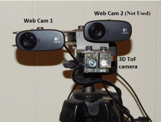
This research both 2D and 3D imaging sensors were utilized to develop a plant
phenotyping system based on a 3D reconstruction scheme. As Figure 1 indicates, two 2D web-cameras were mounted beside a 3D ToF camera to form a sensor assembly, though web-camera-2 was in fact not used in the process. The 3D imaging sensor was used to capture the point cloud data of different parts of the corn plant, and the 2D web-camera-1 was used to capture the image of chessboard pattern targets array simultaneously. This research contributes a method to calibrate the pose relationship between the 2D and 3D
cameras. For each view point, by analyzing the captured 2D images of the chessboard pattern beacon, the 2D camera’s pose related to the beacon can be estimated. Based on the pose of 2D camera and the calibrated relationship between the 2D and 3D cameras, the position and attitude of the 3D sensor related to beacon at the same time can be derived. Then, based on the 3D sensor’s pose corresponding to each point cloud data view, different views can be aligned precisely to reconstruct the complete 3D model.
The depth measurement repeatability of the 3D camera used is 5 mm. It can provide amplitude value, which is the intensity of reflected light, and the x, y, z coordinates for each point. Its standard depth measurement range is 0 to 2 m, according to the datasheet; however, our experiment indicated the best working distance between the object and sensor was between 0.2 and 0.5 m in this research. Since the 3D camera can be placed as close as about 0.2 m to the observed object, the captured point cloud data can provide details of different parts of plant despite its low pixel resolution. In this case, the complete 3D model with detailed information could be obtained.
The 2D camera used to track the 3D camera’s pose is the Logitech HD Webcam C310. It features a wide focus range, 60° field of view, and 1280 x 720 pixel resolution. The distortion effect is satisfactory according to the previous study (Li, 2014). More
importantly, its optical system is fixed. This makes its intrinsic matrix stays the same and can be calibrated, while 2D camera’s intrinsic matrix must be known while applying it to machine vision-based pose estimation application. All of these features indicate it is an appropriate sensor for the 2D imaging based position and attitude system. Before the 2D
camera was used in the experiment, it was calibrated to get its intrinsic matrix and distortion vector based on the theory proposed by Zhang (Zhang, 2000).
Figure 1. Data collection system built for this 3D reconstruction based phenotyping research
Camera Posture Tracking Infrastructure
A beacon array was designed to estimate the position and attitude of the 2D and 3D cameras as Figure 2 indicates. One beacon consists of a chessboard pattern and a column of small rectangles as its id on the right, a complete beacon is marked by the green rectangle of Figure 2. 2D machine vision algorithm was developed to detect the beacon.
The system could precisely estimate the 2D camera’ pose related to beacon by resolving the pinhole model of 2D camera with the coordinates of the detected inner corners of chessboard pattern in the captured image and the coordinate system defined by beacon. Work also has been done to decode beacon’s id. The detail is available in (Li, 2014).
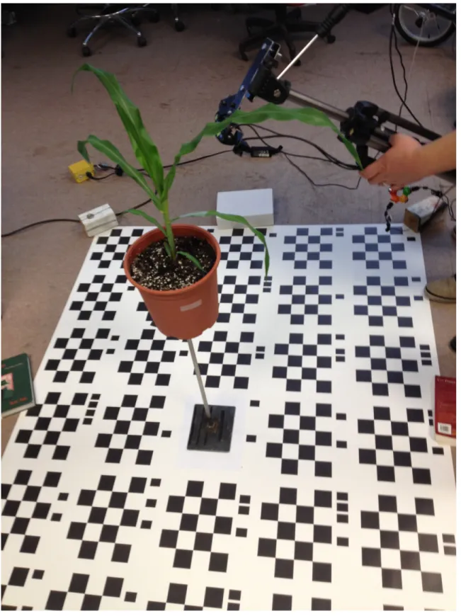
As long as a complete beacon is captured by the 2D camera, its pose can be precisely estimated. With the relationship between 2D and 3D camera, the pose of 3D camera can also be calculated. The target array was designed to contain seven rows by five columns of beacons. By placing the corn plant pot about 0.7 m above the center of the beacon array and holding the data collection system as Figure 3 indicates, the 2D camera can capture at least one complete beacon when the 3D imaging sensors are observing the corn plant at different viewpoints.
The chessboard beacon target defined the world coordinate system of the research platform. As Figure 2 shows, the origin of the world coordinate system is the bottom-left inner corner of the bottom-left beacon in the target array, and its X and Y axis are parallel to the up and right direction of the target array, respectively. In addition, the direction of the Z axis is vertically going inside the target array. In this study, the position and attitude estimation result of the 2D and 3D cameras was related to the world coordinate system.
All of the beacons in the target array have identical chessboard pattern design, and each one consists of 5 × 4 squares, as Figure 2 shows. The side of each square was 52.36 mm. The translation relationship between two neighbor beacons at the same row was [292.72,
0, 0]T mm, and that between the two neighbor beacons at the same column was [0, 303.43, 0]T mm.
The beacon ID was labeled by a column of small rectangles on the right side of each target. When the inner corners of the corresponding beacon were extracted from image, their world coordinates value can be achieved based on target id to estimate the pose of 2D and 3D camera.
Figure 2. World coordinate system and beacon array used as the camera’s pose estimation infrastructure
Position and Attitude Estimation of 3D Camera
To reconstruct the complete 3D model of the corn plant, the position and attitude of the 3D camera corresponding to every point cloud data view are required. The pose of the 3D camera was derived from the pose of the 2D camera plus the position and attitude
relationship between the two cameras. Therefore, the pose estimation of the 2D camera and the calibration of the relationship between the 2D and 3D cameras are critical.
Position and Attitude Estimation of 2D Camera
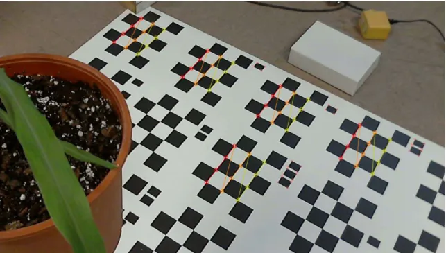
When the 3D ToF camera was collecting the point cloud data of the corn plant, the image of the beacon targets was captured simultaneously by its adjacent 2D imaging sensor. The system extracted the inner corners of chessboard pattern of beacons from the 2D image and recognized beacons’ IDs, as Figure 4a shows. Based on their ID and pre-knowledge of the beacons array, the system achieved the world coordinates of the inner corners of the detected beacons. For every detected inner corner, its coordinates on the 2D image and its world coordinate complies the pinhole mode expressed by Equation 1.
�𝑥𝑥𝑦𝑦 1�= 𝑠𝑠𝑠𝑠[𝑅𝑅 | 𝑡𝑡]� 𝑋𝑋 𝑌𝑌 𝑍𝑍 1 � (1)
Where (x, y) is the image coordinate, and (X, Y, Z) is its corresponding world coordinate;
M is the intrinsic matrix of 2D camera, which is calibrated beforehand; R and t are the rotation matrix and translation vector between 2D camera and the world coordinate system defined by the beacons array; and s is a unknown scale factor.
By inputting the world coordinates and image coordinates pairs of all inner corners of detected beacons and calibrated intrinsic matrix M of 2D camera, rotation matrix R, translation vector t, and scale factor s of Equation 1 can be resolved with regression calculation. In this case, the position and attitude of the 2D camera related to the world coordinate system, which is represented by the rotation matrix R and the translation vector t, is resolved (Li, 2014).
The 2D camera can capture one or more beacons during the data collection process depending on the viewpoint (Figure 4). One detected beacon can provide image
coordinates and world coordinates pairs of 12 inner corners, which are enough to resolve Equation 1 to estimate the pose of 2D camera. The more beacons were detected, the more inner corners can be used in the regression calculation to resolve Equation 1, benefiting the calculation result better robustness to noise and higher numerical stability. In this research, the distance between 2D camera and beacons is between 1 and 2 m. In this condition, the translation measurement error is less than 1 cm and the attitude measurement error is around 1 degree according to our other study (Li, 2014).
(a)
(b)
(c)
Figure 4. Images collected by 2D and 3D camera: (a) chessboard patterns of beacons were detected by 2D camera, and the small rectangles of beacon IDs were extracted, (b)
depth image collected by 3D ToF camera, and (c) intensity image captured by 3D ToF camera
Calibration between 2D and 3D Cameras
In this application calibrated the relationship between the 2D and 3D cameras. The design of the data collection system made it impossible for the 2D camera and the 3D camera to observe the same chessboard target simultaneously. To solve this problem, two
chessboard targets were used and assembled side by side (Figure 5a). The calibration procedure is described below.
First, the relationship between the two chessboard targets was calibrated. The data collection system was moved to a relatively farther viewpoint A, and the 2D camera captured an image that contains two targets (Figure 5a). The system detected two targets and estimated the relationship between the coordinate system of the 2D camera and each target separately. The rotation matrix and the translation vector of the 2D camera’s coordinate system related to the left target are represented with RLA and tLA, respectively, and those related to the right target are represented with RRA and tRA. For a point, Q2D,
Q�L, and Q�R represents its coordinate in the coordinate system of 2D camera, left target,
and right target respectively. The relationship between Q2D, Q�L and Q�R of a same point can be expressed by Equation 2 and 3. In addition, the relationship between the
coordinate systems defined by two targets can be expressed by Equation 4. 𝑄𝑄2𝐷𝐷= 𝑅𝑅𝐿𝐿𝐿𝐿𝑄𝑄�𝐿𝐿+𝑡𝑡𝐿𝐿𝐿𝐿 (2)
𝑄𝑄2𝐷𝐷= 𝑅𝑅𝑅𝑅𝐿𝐿𝑄𝑄�𝑅𝑅 +𝑡𝑡𝑅𝑅𝐿𝐿 (3)
Based on Equation 4, the rotation matrix RL2R and the translation vector tL2R of left target related to right target is expressed by Equation 5 and 6.
𝑅𝑅𝐿𝐿2𝑅𝑅 = 𝑅𝑅𝑅𝑅𝐿𝐿−1𝑅𝑅𝐿𝐿𝐿𝐿 (5)
𝑡𝑡𝐿𝐿2𝑅𝑅 =𝑅𝑅𝑅𝑅𝐿𝐿−1(𝑡𝑡𝐿𝐿𝐿𝐿− 𝑡𝑡𝑅𝑅𝐿𝐿) (6)
Then Equation 4 can be written with other format as Equation 7 indicates. 𝑄𝑄�𝑅𝑅 = 𝑅𝑅𝐿𝐿2𝑅𝑅𝑄𝑄�𝐿𝐿+𝑡𝑡𝐿𝐿2𝑅𝑅 (7)
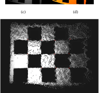
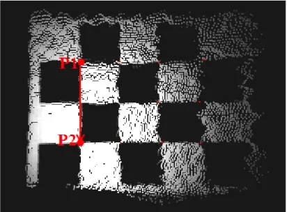
Second, the data collection system was moved closer to two targets, and the position of the data collection system at this time was viewpoint B. At viewpoint B, the 2D camera can only capture the image of the right target as Figure 5b shows, while the 3D ToF camera gets the intensity image and 3D data of the left target as Figure 5c and 5d show. By extracting the right chessboard target from the image captured by the 2D camera as Figure 5b indicates, the rotation matrix RRB and the translation vector tRB of the 2D camera at viewpoint B related to right target can be achieved. Moreover, the rotation matrix RL22D and the translation vector tL22D of the left target related to the 2D camera at viewpoint B can be derived based on Equation 4–7, RRB, and tRB. The derivation results are expressed by Equation 8 and 9.
𝑅𝑅𝐿𝐿22𝐷𝐷 = 𝑅𝑅𝑅𝑅𝑅𝑅𝑅𝑅𝐿𝐿2𝑅𝑅 =𝑅𝑅𝑅𝑅𝑅𝑅𝑅𝑅𝑅𝑅𝐿𝐿−1𝑅𝑅𝐿𝐿𝐿𝐿 (8)
𝑡𝑡𝐿𝐿22𝐷𝐷 = 𝑅𝑅𝑅𝑅𝑅𝑅𝑅𝑅𝐿𝐿2𝑅𝑅𝑡𝑡𝐿𝐿2𝑅𝑅+𝑡𝑡𝑅𝑅𝑅𝑅=𝑅𝑅𝑅𝑅𝑅𝑅𝑅𝑅𝑅𝑅𝐿𝐿−1(𝑡𝑡𝐿𝐿𝐿𝐿 − 𝑡𝑡𝑅𝑅𝐿𝐿) +𝑡𝑡𝑅𝑅𝑅𝑅 (9)
Third, the relationship between the left target and the 3D camera at viewpoint B was estimated. The point cloud data of the chessboard target from the 3D camera was processed by linear regression algorithm to estimate the plane of the target board; and then the original point cloud data were replaced with their projection points on the plane
to reduce the measurement error of the 3D data. Additionally, the inner corners of the left chessboard target were extracted from the intensity image captured by the 3D camera, as Figure 5c shows, to get the inner corners’ coordinate value related to the 3D camera. The relationship between the coordinate systems of the left target and the 3D camera can be estimated based on two steps, as follows:
1) The target plane in the 3D camera’s coordinate system was achieved in the plane regression calculation, and the target plane in its own coordinate system is Z = 0. The rotation matrix𝑅𝑅1 between the target plane in the 3D camera’s coordinate system and the plane Z = 0 was estimated first. The normal
direction of the target plane related to the coordinate system of the target is [0, 0, 1]T , and the normal direction of the target plane related to the 3D camera’s coordinate system is unit vector [a, b, c] T. The value of [a, b, c] T was
achieved in the target plane regression step. The rotation matrix for the rotation from [0, 0, 1]T to [a, b, c] T is 𝑅𝑅
1. The corresponding rotation axis L is
perpendicular to both [0, 0, 1]T and [a, b, c] T; therefore, L is the cross product
of two vectors, as Equation 10 indicates, and the rotation angle is expressed by Equation 11. L =�00 1�×� a b c�=� −b a 0 � (10) θ= arccos � � 0 0 1�∙� a b c� √a2+b2+c2�= arccos (c) (11)
The rotation matrix 𝑅𝑅1 can be derived by applying the Rodrigues’ rotation formula with rotation axis L, and the rotation angle θ; the result is described
by Equation 12.
R1 =�
b2+ a2cos (θ) ba(cos(θ)−1) sin (θ)a ba(cos(θ)−1) a2+ b2cos (θ) sin (θ)b
−sin (θ)a −sin (θ)b (b2+ a2)cos (θ)�
(12)
2) By applying the rotation matrix 𝑅𝑅1 to the 3D camera’s coordinate system 𝐶𝐶3𝑑𝑑, a new coordinate system 𝐶𝐶3𝑑𝑑′ was achieved. The Z axis of 𝐶𝐶3𝑑𝑑′ and the Z axis of the coordinate system of the left target 𝐶𝐶𝐿𝐿 are parallel. Therefore, by rotating the coordinate system 𝐶𝐶3𝑑𝑑′ around its Z axis with an angle β, the X, Y, Z axis of the new coordinate system 𝐶𝐶3𝑑𝑑′′ is parallel to the X, Y, Z axis of coordinate system 𝐶𝐶𝐿𝐿. Figure 6 shows the coordinate system 𝐶𝐶𝐿𝐿 defined by the left target. Point P1 and P2 in Figure 7 are two inner corners of the target. P1 is the origin point of the coordinate system 𝐶𝐶𝐿𝐿, and P2 is on the X axis of 𝐶𝐶𝐿𝐿. The original XYZ coordinate of P1 and P2 provided by the 3D ToF camera are represented by vector V1 and V2, respectively, and the cos(β) and sin(β) can be calculated by Equation 13–15.
𝑉𝑉 =𝑅𝑅1(𝑉𝑉2− 𝑉𝑉1) (13)
where vector V can be presented with [u, w, 0]T.
cos(𝛽𝛽) =𝑉𝑉∙� 1 0 0� |𝑉𝑉| = 𝑢𝑢 √𝑢𝑢2+𝑤𝑤2 (14) sin(𝛽𝛽) =𝑉𝑉×� 1 0 0� |𝑉𝑉| = −𝑤𝑤 √𝑢𝑢2+𝑤𝑤2 (15)
(a)
(c) (d)
(e)
Figure 5. 2D and 3D camera calibration images: (a) images of two chessboard targets captured by 2D camera at a farther viewpoint A, (b) image of right chessboard target captured by 2D camera at close viewpoint B, (c–e) intensity and depth image and point
Figure 6. Coordinate system CL defined by left target board
Figure 7. Inner corner points P1 and P2 on the X axis of the coordinate system defined by the left target board
The rotation matrix R2 from coordinate system 𝐶𝐶3𝑑𝑑′′ to 𝐶𝐶𝐿𝐿 is expressed with Equation 16. 𝑅𝑅2 = � cos (𝛽𝛽) −sin (𝛽𝛽) 0 sin (𝛽𝛽) cos (𝛽𝛽) 0 0 0 1�= � 𝑢𝑢 √𝑢𝑢2+𝑤𝑤2 𝑤𝑤 √𝑢𝑢2+𝑤𝑤2 0 −𝑤𝑤 √𝑢𝑢2+𝑤𝑤2 𝑢𝑢 √𝑢𝑢2+𝑤𝑤2 0 0 0 1 � (16) Having rotation matrix 𝑅𝑅1 and 𝑅𝑅2, the rotation matrix 𝑅𝑅3𝐷𝐷2𝐿𝐿 of coordinate system 𝐶𝐶3𝑑𝑑 related to the coordinate system of left target 𝐶𝐶𝐿𝐿 can be achieved as Equation 17 expresses.
𝑅𝑅3𝐷𝐷2𝐿𝐿 = 𝑅𝑅1𝑅𝑅2 (17)
Finally, the translation vector 𝑡𝑡3𝐷𝐷2𝐿𝐿 of coordinate system 𝐶𝐶3𝑑𝑑 related to the coordinate system of left target 𝐶𝐶𝐿𝐿 can be achieved as Equation 18 expresses. 𝑡𝑡3𝐷𝐷2𝐿𝐿 =−𝑅𝑅3𝐷𝐷2𝐿𝐿𝑃𝑃1 =−𝑅𝑅1𝑅𝑅2𝑃𝑃1 (18)
Fourth, the rotation matrix R3D22D and the translation vector t3D22D from the coordinate system of 3D camera C3d to the coordinate system of 2D camera C2d can be expressed by Equation 19 and 20.
𝑅𝑅3𝐷𝐷22𝐷𝐷 =𝑅𝑅𝐿𝐿22𝐷𝐷𝑅𝑅3𝐷𝐷2𝐿𝐿 (19)
𝑡𝑡3𝐷𝐷22𝐷𝐷 =𝑅𝑅𝐿𝐿22𝐷𝐷𝑡𝑡3𝐷𝐷2𝐿𝐿+𝑡𝑡𝐿𝐿22𝐷𝐷 (20)
For a point, if its coordinates in the coordinate system of the 3D camera and the 2D camera are represented using Q3D and Q2D, respectively, Q3D and Q2D satisfy Equation 21.
𝑄𝑄2𝐷𝐷= 𝑅𝑅3𝐷𝐷22𝐷𝐷𝑄𝑄3𝐷𝐷+𝑡𝑡3𝐷𝐷22𝐷𝐷 (21)
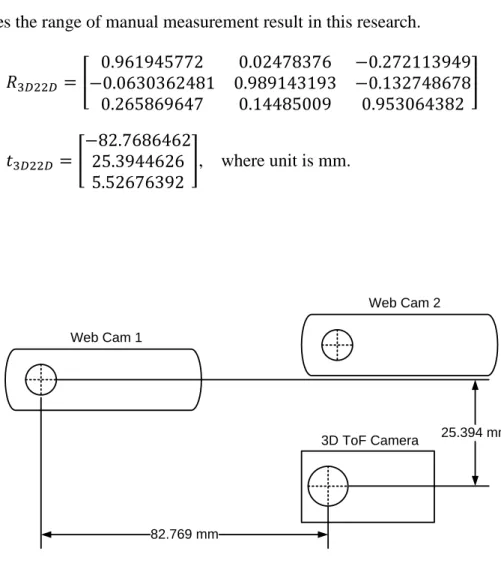
For the data collection system of this research, the value of R3D22D and t3D22D is given by Equation 22 and 23. The distance between the 2D and 3D cameras is |t3D22D|, which
is 86.75 mm according to the value of t3D22D. Their actual horizontal and vertical distances are 82.769 and 25.394 mm. Figure 8 provides the translation relationship between the cameras of the data collection system using the calibration result t3D22D. It matches the range of manual measurement result in this research.
𝑅𝑅3𝐷𝐷22𝐷𝐷 =� 0.961945772 0.02478376 −0.272113949 −0.0630362481 0.989143193 −0.132748678 0.265869647 0.14485009 0.953064382 � (22) 𝑡𝑡3𝐷𝐷22𝐷𝐷 = � −82.7686462 25.3944626 5.52676392 � , where unit is mm. (23) 82.769 mm 25.394 mm Web Cam 1 Web Cam 2 3D ToF Camera
Figure 8. Translation relationship between cameras of the data collection system with calibration result
The 3D camera collects the 3D point cloud data view of different parts of the corn plant, and the 2D camera beside the 3D camera captures the images of beacons simultaneously for pose estimation of the 3D camera corresponding to each point cloud view, as Figure 4 indicates. The 3D reconstruction recovered the complete 3D model of the corn plant through 3D registration, which aligned different point cloud data views together according to the position and attitude of corresponding viewpoints estimated by the 2D camera. In this research, the size of corn plants were V5 to V6 growth stages and it was found that about 20 point clouds would be needed to reconstructed a complete 3D view of the plant. The exact number of point could views needed for a given plant depends on its size and structural complexity.
Preprocessing
Before 3D registration, the preprocessing to clean the noise point of each point cloud data view should be accomplished. Points that qualify any of the following criteria were recognized as noise and were removed.
1) The point whose amplitude value is too high is identified as noise by the PMD camera. It happens where the ambient light is too strong for the light source of PMD camera to achieve valid 3D information.
2) The point with depth over 0.7 m, because the interested object is always within 0.7 m in front of the 3D camera.
3) In the 3D space, the sparse point which has less than a specific number of neighbor points within the defined radius was treated as noise and removed. In
this research the radius value was selected as 10 mm, and the neighbor point count threshold was set as 12. Sparse point cleaning was critical to get clean 3D image views for 3D reconstruction as Figure 9 shows.
(a)
(b)
Figure 9. (a) The 3D model’s achievement without sparse point noise clearance and (b) the 3D model’s achievement with sparse noise clearance
3D Registration
As Figure 4 shows, the 2D camera of the data collection system captures the 2D images of chessboard targets simultaneously when the 3D camera collects the point cloud view. As discussed previously, with the world coordinate value of the inner corners of detected targets, the system estimates the rotation matrix R2D and the translation vector t2D of the 2D camera related to the world coordinate system defined by target array by resolving the pinhole model of 2D camera. For a point in 3D space, its 3D coordinate vector Q2D
related to the 2D camera and its coordinate related to target array Qw should satisfy Equation 24.
𝑄𝑄2𝐷𝐷= 𝑅𝑅2𝐷𝐷𝑄𝑄𝑤𝑤+𝑡𝑡2𝐷𝐷 (24)
Based on the relationship between the 2D and 3D cameras, the 3D coordinate vector Q3D of the point cloud data view from the 3D camera can be converted to the coordinate values related to the world coordinate system as Equation 25 describes based on Equation 21 and 24.
𝑄𝑄𝑤𝑤 = 𝑅𝑅2𝐷𝐷−1(𝑅𝑅3𝐷𝐷22𝐷𝐷𝑄𝑄3𝐷𝐷+𝑡𝑡3𝐷𝐷22𝐷𝐷− 𝑡𝑡2𝐷𝐷) (25)
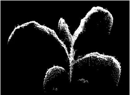
For each 3D point cloud view, the position and attitude of the 3D camera vary. However, the world coordinate system defined by the target array is consistent because the plant and target array keep static during the data collection process. By applying Equation 25 to convert the original 3D information of different point cloud data views from the ToF camera to those related to the consistent world coordinate system, the 3D registration is done. Figures 10a and b shows the side view and top view of a 3D model reconstruction of a corn plant. It was obtained by aligning 23 point cloud data views together. Among all
of the 23 data views, one is shown with green color points in Figures 10a and b, and its intensity and depth image are provided by Figures 10c and d.
(a)
(b)
(c) (d)
Figure 10. Complete 3D model of corn plant achieved through 3D registration: (a) side view and (b) top view of 3D model, (c) the intensity and (d) depth image of the point
Leaf and Stem Segmentation
After obtaining the 3D model of the corn plant, this research separated leaves and stem in order to measure their physical parameters.
Stem Segmentation
Stem segmentation was carried out first by generating six 2D side view images of a corn plant based on the 3D model as Figure 11 shows. Suppose the range of x, y, and z
coordinate value of the 3D model are [x0, x1], [y0, y1], and [z0, z1], the width and height of the 2D side view image are W and H. The ith side view image is achieved by setting its point (u, v) and corresponding every point of the 3D model to white, and the
relationship between (u, v) of the side view image and the point (x, y, z) of the 3D model is expressed by Equation 26–28.
𝜑𝜑 =𝑖𝑖 ∗60, 𝑤𝑤ℎ𝑒𝑒𝑒𝑒𝑒𝑒𝑖𝑖 ∈{0, 1, 2, 3, 4, 5} (26) 𝑢𝑢 = 0.4��𝑥𝑥 −𝑥𝑥0+𝑥𝑥12 �sin(𝜑𝜑) +�𝑦𝑦 −𝑦𝑦0+𝑦𝑦12 �cos(𝜑𝜑)�+𝑊𝑊2 (27) 𝑣𝑣= 0.4�𝑧𝑧 −𝑧𝑧0+𝑧𝑧12 �+𝐻𝐻2 (28)
For each side view image, this system searched for the straight lines with the length over the threshold and the angle around the vertical direction. Pixels on these detected straight lines are displayed with red color in the side view images provided in Figure 11. The points of the 3D model whose corresponding points in all 2D side view image that were on the detected straight lines were recognized as the stem of the corn plant.
(a) (b)
Figure 11 continued
(e) (f)
Figure 11. The stem detected in different side views at different viewpoints
Leaf Segmentation
The stem segmentation obtained in the previous section separated the 3D model into several regions in 3D space, and each big region is one leaf. An efficient 2D image processing-based algorithm was developed to process multiple side views and top view images for region separation in 3D space. Its main idea is to do region separation with different projection view in 2D space of the 3D reconstruction of corn plant. Figure 11 shows an example of side view images, and Figure 12 is the top view image. The
detected stem is displayed with red color in these images. The leaves were separated into different parts by the stem in these projection views in 2D space (Figures 11, 12). For the
point cloud of one leaf, it cannot be divided into different regions by the stem in any projection view. For the point cloud of different leaves, although they may connect as one region for some projection views, they still can be separated apart in the rest ones. The leaf segmentation algorithm based on 2D image processing was developed based on above fact. It started from separating the white points of the first image view by the extracted stem, into regions in 2D space, and the corresponding points of the 3D
reconstruction model were organized into different groups accordingly. Then the system repeated this method to process the next image to check whether the points grouped together previously should be separated into different regions according to this projection view. This procedure was iterated until all the projection views were processed. For the final regions, those whose sizes were smaller than 40 points were removed as noise data in this research, and each of the remaining regions was recognized as a leaf. The stem and leaves of the 3D reconstruction model of the corn plant are well segmented by this
Figure 12. The top view image of the point cloud of the 3D model; the stem is marked with red color
Leaf Parameter Estimation
After the points of the stem and every leaf of 3D reconstruction model were determined, this system was ready to estimate the physical parameters of the corn plant. This research developed the algorithm to estimate the collar height as well as the width, length, and area of leaves.
Leaf Points Regression
To begin the physical parameter estimation of leaves, this research employed Equations 29 and 30 to describe the curve of the skeleton of each leaf. In these two equations, x, y, and z are the known world coordinate value of the skeleton point of the corresponding
leaf. Variables φ, a, b, c, d, and e of these two equations are unknown, and they are
solved by applying singular value decomposition (SVD) regression method to process the 3D information of all points of the corresponding leaf.
𝑦𝑦�= 𝑥𝑥sin(𝜑𝜑) +𝑦𝑦cos(𝜑𝜑) (29) 𝑧𝑧=𝑎𝑎𝑦𝑦�4+𝑏𝑏𝑦𝑦�3+𝑐𝑐𝑦𝑦�2+𝑑𝑑𝑦𝑦�+𝑒𝑒 (30)
Leaf Parameter Estimation
Having φ solved, Equation 29 was applied to calculate y� value of every point of the corresponding leaf. The white pixels of Figure 13 show the transformation result of leaf 3 in Figure 17(a). For Figure 13, the horizontal direction linearly related to y� value of the point, and vertical direction related to its z value. The red curved line shows the
polynomial regression result represented by Equation 30, and the white part is the point cloud of the corresponding leaf. Moreover, Equation 31 was used to calculate x� value of all of the point of the corresponding leaf.
𝑥𝑥�= 𝑥𝑥cos(𝜑𝜑)− 𝑦𝑦sin(𝜑𝜑) (31)
Based on the leaf skeleton curve described by the solved Equation 30, the leaf length and area was estimated. The range of y� value of a leaf is represented with [y�min, y�max]. To estimate the length and area of the leaf, the leaf was divided into 50 fractions along the direction parallel to the x� axis. In addition, the ith fraction, which is represented with Fi in this research, contains all of the points whose y� is within the range between Y�i−1 and Y�i, where Y�i is represented by Equation 32.
Then by applying y� = Y�i to Equation 30, the corresponding result value z is represented with Z�i.
Figure 13. Regression result of leaf 3 of plant 1
Then the leaf length is achieved using Equation 33.
𝐿𝐿𝑒𝑒𝐿𝐿𝐿𝐿𝑡𝑡ℎ= ∑50𝑖𝑖=1�(𝑌𝑌�𝑖𝑖− 𝑌𝑌�𝑖𝑖−1)2+ (𝑍𝑍�𝑖𝑖− 𝑍𝑍�𝑖𝑖−1)2 (33)
Additionally, if the minimum and maximum x� value of the points of Fi are represented with x�imin and x�imax, their difference is the width of fraction Fi. In addition, the area and width of the leaf can be achieved as shown in Equations 34 and 35:
𝑎𝑎𝑒𝑒𝑒𝑒𝑎𝑎=∑50𝑖𝑖=1��(𝑌𝑌�𝑖𝑖 − 𝑌𝑌�𝑖𝑖−1)2+ (𝑍𝑍�𝑖𝑖 − 𝑍𝑍�𝑖𝑖−1)2× (𝑥𝑥�𝑖𝑖𝑖𝑖𝑖𝑖𝑥𝑥− 𝑥𝑥�𝑖𝑖𝑖𝑖𝑖𝑖𝑖𝑖)� (34)
𝑤𝑤𝑖𝑖𝑑𝑑𝑡𝑡ℎ= max(𝑥𝑥�𝑖𝑖𝑖𝑖𝑖𝑖𝑥𝑥− 𝑥𝑥�𝑖𝑖𝑖𝑖𝑖𝑖𝑖𝑖) 𝑖𝑖 ∈{0, 1, 2, … … , 50}. (35)
The leaf collar height was also estimated. As the coordinate of the point cloud of the 3D reconstruction model is related to the world coordinate system defined by the target array on the ground, the Z coordinate of a point actually is its height from the ground. The leaf
collar was located by finding the conjunction point between the stem and the leaf
skeleton in 3D space. The leaf collar height is the difference between the Z coordinate of the conjunction point in the world coordinate system and the height measurement result of the soil surface of the pot related to the ground.
Results and Discussion
Three corn plants at vegetative stage V5 were used to test this system. The plants were around half a meter and they had seven leaves.
Figures 14–16 are the 2D color pictures and the corresponding 3D reconstruction results of the three corn plants. As they indicate, this system achieved a relatively clean and complete 3D model of the corn plant. Visually, the 2D color images and 3D
reconstruction result match well together. However, the 3D reconstruction images show that the bottom one or two leaves of corn plants were either missed or incomplete in the reconstruction. Noisy 3D information of the bottom leaves caused by their small sizes led to the incomplete reconstruction. Additionally, the reflectance of the soil surface of the pot to the light source of the 3D camera was very low, which resulted in noisy 3D data. The noisy 3D data of the soil surface fused with the point cloud of the bottom leaves, making it difficult to extract bottom leaves. Therefore, part or whole of bottom leaves were removed as noise.
Figure 17 provides the leaf and stem separation result of the 3D reconstruction of three corn plants. The leaves and stem are accurately separated, and they are displayed with different color in the result images. The IDs of different leaves are also given by Figure 17.
To quantitatively evaluate the accuracy of the 3D model, this system estimated the parameters of each leaf of every plant, including width, length, area, and collar height, which were compared with the reference measurement results. The leaves’ area
measurement result provided by LI-3100C Leaf Area Meter was used as the ground true value, and the other three parameters were measured manually. The parameters measured by this system and by the reference methods are listed in Tables 1–3. The corresponding error rate is also listed. For the bottom one or two leaves of corn plants, the measurement results of this system are not available because they were missed in their 3D
reconstruction model.
Statistical analysis was conducted for the measurement of error rate (Table 4). As it indicates, the median value of each parameter’s error rate is smaller than 7.18%. The average measurement error rate of a leaf’s area, length, width, and collar height are 10.46%, 10.42%, 11.10%, and 8.18%, respectively. The third quartile value of these measurement errors are 11.14%, 11.75%, 13.48%, and 6.88%. Therefore, a big part of the measurement has reasonable accuracy. However, there are some big outliers for each parameter’s measurement. For instance, the error rate of width and area measurement of leaf 1 of plant 2 is 41.2% and 31.13%, respectively. Another example is that the area and length measurements of leaf 5 of plant 2 are 61.87% and 27.55% smaller than the
reference value, which is because this leaf is too small for the ToF camera, thus causing incomplete reconstruction.
When running on a 3.4 GHz Intel Xeon CPU, the system’s average processing time cost for 3D reconstruction and leaf parameter estimation of a corn plant was 4.73 second. The processing time cost for a corn plant was less or at least comparable to the time needed to move the imaging sensor to around 20 viewpoints to collect different point cloud data views. Therefore, the image data processing and image collection process can be performed simultaneously.
(a)
(b)
Figure 14. Corn plant 1 and its 3D reconstruction result: (a) 2D color picture and (b) 3D reconstruction result
(a)
(b)
Figure 15. Corn plant 2 and its 3D reconstruction result: (a) 2D color picture and (b) 3D reconstruction result
(a)
(b)
Figure 16. Corn plant 3 and its 3D reconstruction result: (a) 2D color picture and (b) 3D reconstruction result
(a)
(c)
Figure 17. Leaf and stem segmentation result: (a) plant 1, (b) plant 2, and (c) plant 3
Conclusions
In this research, a 3D reconstruction-based phenotyping system of plant was developed. The results of the study revealed that this system exhibited promising potential for developing a maize phenotyping system.
The 3D reconstruction approach is effective. The chessboard pattern target array can provide precise position and attitude estimation of the 2D camera. Moreover, the proposed calibration method was proven effective in getting the spatial relationship between the 2D and 3D cameras, which were installed side by side as the data capturing system of this study, and therefore enabled deriving the pose of the 3D camera in the
world coordinate system based on that of the 2D camera. According to the position and attitude of the 3D camera corresponding to each 3D image view, different views were aligned precisely into a complete 3D reconstruction of a corn plant.
It can also be concluded that the processing algorithm of the reconstructed 3D model of the corn plant is promising. The segmentation algorithm was effective to extract the stem and each leaf from the 3D model of the corn plant. Leaf points regression and leaf
parameter estimation algorithms automatically quantified the leaf phenotypic parameters, such as leaf width, leaf length, leaf area, and collar height. The measurement of the leaf parameter is promising, though outliers still exist.
The fast processing speed, high accuracy, low cost, and nondestructive nature of this phenotyping system may benefit any high-throughput phenotyping system that can collect and process data throughout the life cycle of plants.
Reference
1. Alenya, G., Dellen, B., Torras, C., 2011. 3D modelling of leaves from color and tof data for robotized plant measuring, 2011 IEEE International Conference on Robotics and Automation. IEEE, Shanghai, China, pp. 3408-3414.
2. Allen, H.L., Estrada, K., Lettre, G., Berndt, S.I., Weedon, M.N., Rivadeneira, F., Willer, C.J., Jackson, A.U., Vedantam, S., Raychaudhuri, S., 2010. Hundreds of variants clustered in genomic loci and biological pathways affect human height.
Nature 467, 832-838.
3. Bellasio, C., Olejníčková, J., Tesař, R., Šebela, D., Nedbal, L., 2012. Computer reconstruction of plant growth and chlorophyll fluorescence emission in three spatial dimensions. Sensors 12, 1052-1071.
4. Chaerle, L., Lenk, S., Leinonen, I., Jones, H.G., Van Der Straeten, D., Buschmann, C., 2009. Multi-sensor plant imaging: Towards the development of a stress-catalogue. Biotechnology Journal 4, 1152-1167.
5. Cobb, J.N., DeClerck, G., Greenberg, A., Clark, R., McCouch, S., 2013. Next-generation phenotyping: requirements and strategies for enhancing our understanding of genotype–phenotype relationships and its relevance to crop improvement. Theoretical and Applied Genetics 126, 867-887.
6. Fiorani, F., Rascher, U., Jahnke, S., Schurr, U., 2012. Imaging plants dynamics in heterogenic environments. Current opinion in biotechnology 23, 227-235.
7. Foundation, N.S., Mcb, G., 2011. Phenomics : Genotype to Phenotype A report of the Phenomics workshop sponsored by the USDA and NSF.
8. Fredriksson, L., 2011. Evaluation of 3D reconstructing based on visual hull algorithms.
9. Furbank, R.T., Tester, M., 2011. Phenomics - technologies to relieve the phenotyping bottleneck. Trends in Plant Science 16, 635-644.
10.Granier, C., Aguirrezabal, L., Chenu, K., Cookson, S.J., Dauzat, M., Hamard, P., Thioux, J.J., Rolland, G., Bouchier-Combaud, S., Lebaudy, A., Muller, B., Simonneau, T., Tardieu, F., 2006. PHENOPSIS, an automated platform for reproducible phenotyping of plant responses to soil water deficit in Arabidopsis
thaliana permitted the identification of an accession with low sensitivity to soil water deficit. New Phytologist 169, 623-635.
11.Heffner, E.L., Jannink, J.-L., Sorrells, M.E., 2011. Genomic selection accuracy using multifamily prediction models in a wheat breeding program. The Plant Genome 4, 65-75.
12.Jansen, M., Gilmer, F., Biskup, B., Nagel, K.A., Rascher, U., Fischbach, A., Briem, S., Dreissen, G., Tittmann, S., Braun, S., De Jaeger, I., Metzlaff, M., Schurr, U., Scharr, H., Walter, A., 2009. Simultaneous phenotyping of leaf growth and chlorophyll fluorescence via GROWSCREEN FLUORO allows detection of stress tolerance in Arabidopsis thaliana and other rosette plants. Functional Plant Biology 36, 902-914.
13.Klodt, M., Cremers, D., 2014. High-resolution plant shape measurements from multi-view stereo reconstruction, European Conference on Computer Vision. Springer, pp. 174-184.
14.Kumar, P., Connor, J., Mikiavcic, S., 2014. High-throughput 3D reconstruction of plant shoots for phenotyping, Control Automation Robotics & Vision (ICARCV), 2014 13th International Conference on. IEEE, pp. 211-216.
15.Li, J., 2014. 3D machine vision system for robotic weeding and plant phenotyping.
16.Lu, Y., Savage, L.J., Larson, M.D., Wilkerson, C.G., Last, R.L., 2011. Chloroplast 2010: a database for large-scale phenotypic screening of Arabidopsis mutants. Plant physiology 155, 1589-1600.
Kazmierczak, K.M., Lee, K.J., Wong, A., 2011. Phenotypic landscape of a bacterial cell. Cell 144, 143-156.
18.Pound, M.P., French, A.P., Murchie, E.H., Pridmore, T.P., 2014. Automated recovery of three-dimensional models of plant shoots from multiple color images. Plant Physiology 166, 1688-1698.
19.Rusu, R.B., Blodow, N., Marton, Z.C., Beetz, M., 2008. Aligning point cloud views using persistent feature histograms, Intelligent Robots and Systems, 2008. IROS 2008. IEEE/RSJ International Conference on. IEEE, pp. 3384-3391.
20.Scholes, J.D., Rolfe, S.A., 2009. Chlorophyll fluorescence imaging as tool for understanding the impact of fungal diseases on plant performance: a phenomics perspective. Functional Plant Biology 36, 880-892.
21.Sirault, X.R.R., James, R.A., Furbank, R.T., 2009. A new screening method for osmotic component of salinity tolerance in cereals using infrared thermography. Functional Plant Biology 36, 970-977.
22.Song, Y., Glasbey, C.A., Polder, G., van der Heijden, G.W.A.M., 2014. Non-destructive automatic leaf area measurements by combining stereo and time-of-flight images. IET Computer Vision 8, 391 – 403.
23.Speliotes, E.K., Willer, C.J., Berndt, S.I., Monda, K.L., Thorleifsson, G., Jackson, A.U., Allen, H.L., Lindgren, C.M., Luan, J.a., Mägi, R., 2010. Association analyses of 249,796 individuals reveal 18 new loci associated with body mass index. Nature genetics 42, 937-948.
24.Swarbrick, P.J., Schulze-Lefert, P., Scholes, J.D., 2006. Metabolic consequences of susceptibility and resistance (race-specific and broad-spectrum) in barley
leaves challenged with powdery mildew. Plant Cell and Environment 29, 1061-1076.
25.Walter, A., Scharr, H., Gilmer, F., Zierer, R., Nagel, K.A., Ernst, M., Wiese, A., Virnich, O., Christ, M.M., Uhlig, B., Juenger, S., Schurr, U., 2007. Dynamics of seedling growth acclimation towards altered light conditions can be quantified via GROWSCREEN: a setup and procedure designed for rapid optical phenotyping of different plant species. New Phytologist 174, 447-455.
26.Ward, B., Bastian, J., Hengel, A.v.d., Pooley, D., Bari, R., Berger, B., Tester, M., 2015. A model-based approach to recovering the structure of a plant from images. arXiv preprint arXiv:1503.03191.
27.Winzeler, E.A., Shoemaker, D.D., Astromoff, A., Liang, H., Anderson, K., Andre, B., Bangham, R., Benito, R., Boeke, J.D., Bussey, H., 1999. Functional characterization of the S. cerevisiae genome by gene deletion and parallel analysis. Science 285, 901-906.
28.Zhang, Z., 2000. A flexible new technique for camera calibration. IEEE Transactions on pattern analysis and machine intelligence 22, 1330-1334.
29.Figure Caption
Figure 1. Data collection system built for this 3D reconstruction based phenotyping research
Figure 2. World coordinate system and beacon array used as the camera’s pose estimation infrastructure
Figure 3. Infrastructure setup
Figure 4. Images collected by 2D and 3D camera: (a) chessboard patterns of beacons were detected by 2D camera, and the small rectangles of beacon IDs were extracted, (b) depth image collected by 3D ToF camera, and (c) intensity image captured by 3D ToF camera
Figure 5. 2D and 3D camera calibration images: (a) images of two chessboard targets captured by 2D camera at a farther viewpoint A, (b) image of right chessboard target captured by 2D camera at close viewpoint B, (c–e) intensity and depth image and point cloud data of left chessboard target captured by 3D camera at close viewpoint B
Figure 6. Coordinate system CL defined by left target board
Figure 7. Inner corner points P1 and P2 on the X axis of the coordinate system defined by the left target board
Figure 8. Translation relationship between cameras of the data collection system with calibration result
Figure 9. (a) The 3D model’s achievement without sparse point noise clearance and (b) the 3D model’s achievement with sparse noise clearance
Figure 10. Complete 3D model of corn plant achieved through 3D registration: (a) side view and (b) top view of 3D model, (c) the intensity and (d) depth image of the point cloud data view corresponding to the green points in (a) and (b)
Figure 11. The stem detected in different side views at different viewpoints
Figure 12. The top view image of the point cloud of the 3D model; the stem is marked with red color
Figure 13. Regression result of leaf 3 of plant 1
Figure 14. Corn plant 1 and its 3D reconstruction result: (a) 2D color picture and (b) 3D reconstruction result
Figure 15. Corn plant 2 and its 3D reconstruction result: (a) 2D color picture and (b) 3D reconstruction result
Figure 16. Corn plant 3 and its 3D reconstruction result: (a) 2D color picture and (b) 3D reconstruction result