Indirect Inference for Stochastic Volatility Models via the Log-Squared Observations

ABSTRACT

An indirect estimator of the stochastic volatility (SV) model with AR(1) log-volatility is proposed. The estimator is derived as an application of the method of indirect inference (Gouriéroux, Monfort and Renault (1993)), using an auxi-liary SV model that mimics the SV model of interest (which has latent volatility) but is constructed so as to make volatility observable. The resulting estimator works by fitting an AR(1) to the log-squared observations and then applying a simple transformation to the parameter estimates. A closed-form expression for the asymptotic covariance matrix of the estimator is also derived. The esti-mator is applied to the Brussels All Shares Price Index from January 1, 1980, to January 16, 2003.

Tijdschrift voor Economie en Management Vol. XLIX, 3, 2004

Indirect Inference for Stochastic

Volatility Models via the Log-Squared

Observations

Geert Dhaene

KULeuven, Departement Economi-sche Wetenschappen. Centrum voor Economische Studiën, Onderzoeks-groep Econometrie, Leuven.

* I thank the referee for helpful comments. Financial support from FWO research project G.0366.01 is gratefully acknowledged.

I. INTRODUCTION

The phenomenon of volatility clustering is one of the most strik-ing features of financial markets. While short-term returns on financial investment are typically uncorrelated over time and are found to be unpredictable, i.e. have a constant conditional mean given the past observations, there is overwhelming empirical evi-dence that the return variances are positively autocorrelated and predictable, i.e. the returns have a conditional variance that de-pends on past observations. Given the fundamental role that return variances and covariances play in portfolio management and asset pricing, it is important to understand their dynamic behaviour. At present, two classes of models have the inherent property of producing time-varying volatility, along with other phenomena often found in financial time series. The most pop-ular of these is the class of (G)ARCH (Engle (1982); Bollerslev (1986)) and E-GARCH models (Nelson (1991)), which have the attractive feature of being easy to estimate. In these models, the return variance is driven by past shocks (essentially, the residu-als) in the mean equation. By contrast, in SV models, which were introduced by Clark (1973) and extended by Tauchen and Pitts (1983), the return variance is modeled as a separate stochastic process, thus making the return variance a dynamic latent vari-able. As a result, SV models are much harder to estimate and have been used much less in applications. Following an impor-tant paper by Hull and White (1987), in which SV models appear as discrete time approximations to the continuous time volatility diusions used in option pricing theory, there has been a renewed interest in SV models.

Considerable eort has been devoted to developing feasible techniques for estimating SV models. Taylor (1986) and Melino and Turnbull (1990) proposed GMM estimation based on the moments and autocovariances of the absolute returns. Jacquier, Polson and Rossi (1994), Andersen and Sørensen (1996, 1997) and Andersen, Chung and Sørensen (1999) used Monte Carlo methods to study the properties of these estimators. Other avail-able estimation techniques for SV models include quasi-maximum likelihood (Nelson (1988); Harvey, Ruiz and Shephard (1994);

Ruiz (1994)), simulated maximum likelihood (Danielsson and Richard (1993); Danielsson (1994)), simulation-based GMM (Duf-fie and Singleton (1993)), indirect inference (Gouriéroux, Monfort and Renault (1993); Monfardini (1998)), Markov chain Monte Carlo methods (Jacquier, Polson and Rossi (1994); Kim, Shep-hard and Chib (1998); Chib, Nardari and ShepShep-hard (2002)), ef-ficient method of moments (Gallant, Hsieh and Tauchen (1997); Andersen, Chung and Sørensen (1999)), ML Monte Carlo (Sand-mann and Koopman (1998)) and (approximate) maximum likeli-hood (Fridman and Harris (1998)). With the exception of GMM and quasi-maximum likelihood, all of the existing methods re-quire extensive numerical simulation and/or integration. Fur-thermore, obtaining accurate standard errors is far from simple, even with GMM (where the usual standard errors are found to be imprecise) or quasi-maximum likelihood (which involves the Kalman filter as an intermediary step in constructing the quasi-likelihood).

In this paper, a very simple estimator of the basic SV model is presented. In contrast with all existing estimators, closed-form expressions for the estimator and its asymptotic variance are obtained. The estimator is obtained by applying the method of indirect inference (Gouriéroux, Monfort and Renault (1993)) to an auxiliary SV model in which volatility is no longer latent, and then inverting the parameter estimates of the auxiliary model back to the parameters of the original SV model. The particular choice of auxiliary model allows all steps required in the indirect inference procedure to be carried out analytically.

The basic SV model is presented in Section II, along with its main characteristics. Section III briefly outlines the indirect inference approach and then applies it to the model at hand. In Section IV, the estimation method is illustrated with an applica-tion to the Brussels All Shares Price Index. Secapplica-tion V concludes. The more technical derivations are given in the Appendix.

II. THE SV MODEL

In the basic SV model, the time series |1> ===> |W is generated by

|w=hkw@2xw> w= 1> ===> W> (1)

kw+1=+!(kw) +

p

2(1!2)yw> (2)

k₁Q(> 2)> (3)

wherexwandyware standard normal variates, assumed to be

mu-tually independent, independent of k₁ and independent across time, where k1> ===> kW is a latent (i.e. unobserved) time series,

and where !> and 2 are parameters.1 In financial applica-tions, |w is typically the return in periodw on a financial

invest-ment. The essential characteristic of the model is that the vari-ance (i.e. the volatility) of|wis governed by a separate stochastic

process, which is given by (2)—(3). To see this more clearly, ob-serve that the independence of xw and yw31> yw32> === implies the independence ofxwand kw. Therefore, the conditional mean and

variance of|w, givenkw, are

H[|w|kw] =hkw@2H[xw] = 0 (4) and Var [|w|kw] =H £ |w2|kw ¤ =hkw_H£_x2 w ¤ =hkw ₍₅₎

for all w. Note also that|w|kw Q(0> hkw). Thus, the conditional

mean of |w is identically zero, and log (Var [|w|kw]) = kw, i.e.kw

is the log-volatility of |w. The so-called mean equation (1) sets

|w equal to a standard normal variatexw times the standard

de-viation hkw@2_{. Equation (2) specifies the log-volatility to be an}

AR(1) with autoregressive parameter !, unconditional mean and unconditional variance 2. Equation (3) starts the autore-gression of kw by a draw from its stationary distribution. It is

assumed that |!| ? 1, thus ensuring that kw (hence also |w) is

1_{It is more common to parameterise the model in terms of!,=(13!)}

and$=p2_(13!2_{). I prefer the parameterisation in terms of!,and}2

for algebraic reasons and because of a parameter invariance result presented below.

stationary. The unconditional mean and variance of|w are2 H[|w] = 0 and Var [|w] =H h hkwi_=h+1₂2₌

The latter equation follows from the well known property that kwQ(> 2) implies H

£

hkw¤u _=H£_hukw¤_=hu+1₂u22 _{for any u.}

This property of the lognormal distribution will be used through-out the paper. The random variables xw and yw are sometimes

called mean shocks and volatility shocks, respectively. The pres-ence of a separate stochastic component yw governing volatility

(whence the name SV) constitutes the major dierence of SV models relative to GARCH models. The latter class of models replace (2) by a specification in whichkw+1 depends onxw (and,

possibly, on lags of kw and xw) rather than on yw. On the other

hand, GARCH and SV models do share a number of important properties that are often found in financial time series data. First, there is no serial correlation in|w, since

Cov [|w> |w3s] =H[|w|w3s] =H

h

h(kw+kw3s)@2i_H[x

w]H[xw3s] = 0

for any positive integers. Secondly, there is serial correlation in |2_w. To see this, note that Cov(kw> kw3s) = !s2, yielding kw+

kw3sQ(2>22(1 +!s)). So, Cov£|2_w> |2_w3s¤=H£|_w2|_w3s2 ¤H£|_w2¤H£|_w3s2 ¤ =Hhhkw+kw3s i H£x2_w¤H£x2_w3s¤h2+2 =h2+2(1+!s)h2+2= For positive !,Cov£|w2> |w3s2

¤

A 0 for any s. Positive serial cor-relation in |w2, coupled with the absence of serial correlation in

|w, is called volatility clustering, a phenomenon often observed

2

A constant can be added to the right hand side of (1) ifH[|w] = 0 is

judged to be unrealistic. Equivalently, the time series |w can first be

in financial time series, where large returns of either sign tend to cluster together, as do small returns of either sign. Thirdly,

H£|4_w¤ (Var [|w])2 = H£h2kw¤_H£_x4 w ¤ h2+2 = h2+22 _·3 h2+2 = 3h 2 _A3>

which shows that|w has excess kurtosis.

From the point of view of inference, the fundamental problem with the SV model is the latent character of kw, which makes it

di!cult to compute the values of the likelihood function and hence to estimate the parameters by maximum likelihood (ML). To see this, write the joint density of|₁> ===> |W andk1> ===> kW as

i(|1> ===> |W> k1> ===> kW) =i(k1> ===> kW)i(|1> ===> |W|k1> ===> kW) =i(k1) Ã _W Y w=2 i(kw|kw31) ! Ã _W Y w=1 i(|w|kw) ! = Now, i(k₁) =¡22¢31@2h3(k13)2@(22)_> i(kw|kw31) = £ 22(1!2)¤31@2h3[kw33!(kw313)]2@[22(13!2)]_> i(|w|kw) = ³ 2hkw´31@2_h3|w2@(2hkw)₌ So, i(|1> ===> |W> k1> ===> kW) = (2)3W(1!2)3(W31)@2h312 PW w=1kw ×h3(k13)2@(22)3PW_w=2[kw33!(kw313)]2@[22(13!2)] ×h3PWw=1|2w@(2hkw)=

The likelihood function is the joint density of the observables |₁> ===> |W as a function of the parameters, i.e.

O(!> > 2||1> ===> |W) =i(|₁> ===> |W) = Z " 3" === Z " 3" i(|1> ===> |W> k1> ===> kW) gk1 === gkW=

III. INDIRECT INFERENCE

Thus, the likelihood function involves a W-dimensional integral. This integral is not known to be expressible in terms of known mathematical functions. At present, numerical evaluation of the exact likelihood function in not feasible, because with the present speed of computers numerical integration is only possible over low-dimensional spaces, whereas in applicationsW is often large. In the next section, evaluation of the exact likelihood is avoided by recurrence to an auxiliary model which is easy to estimate, and whose parameter estimates can be transformed to yield estimates of!,and 2.

When the parameter vectorof a parametric modelPis di!cult to estimate by ML, indirect inference (Gouriéroux, Monfort and Renault (1993)) may be a feasible alternative to ML. The method involves the following steps:

• Estimate the parameter W of an auxiliary model PD. Let ˆ

W be the estimate.

• Calculate the probability limit ofˆW underP, as a function

of . This gives plim ˆW =W =W(). For identification, it

is assumed that G= _CC0W() has full column rank. • For a given non-stochastic positive definite weighting

ma-trix Z, solve min ³ W()ˆW ´₀ Z ³ W()ˆW ´ =

The solution, , is the indirect estimator ofˆ .

• Calculate the asymptotic covariance matrix ˆas Y = (G0Z G)31G0Z YWZ G(G0Z G)

31_{> (6)}

Remarks:

• The functionW(·), sometimes called the pseudo-true value

function or binding function, links the parameter W to .

It is assumed thatW(·)exists, i.e. that it has a well-defined

probability limit for all. For identification, W(·) must be injective, so it is required thatdim(W)dim().

• The optimal weighting matrix, which gives the smallestY,

isZ =Y3_W1, in which caseY= (G0Y3_W1G)31.

• When dim(W) = dim(), ˆ does not depend on Z and

is equal to 3W1(ˆW), the inverse of the pseudo-true value

function atˆW. In this case,Y =G31YW(G

31₎0_.

• The weighting matrix Z and the pseudo-true value func-tionW(·)may be replaced by consistent estimates without

aecting the asymptotic properties of .ˆ

Indirect inference will now be applied to estimate the parame-ter vector= (!> > 2)0 of modelP, wich is defined by (1)—(3). As auxiliary modelPD, consider the SV model

|w=hkw@2w> (7)

kw+1 =W+!W(kwW) +

p

W2(1!2W)yw> (8)

k1 Q(W> W2)> (9)

wherewandyware mutually independent, independent ofk1 and independent across time, yw is standard normal, w is a

symmet-ric Bernoulli variate with Pr[w = 1] = Pr[w = 1] = 1@2, and

W = (!W> W> 2W)0 is the parameter vector. The only dierence

between this and the original SV model is that the normal vari-ate xw in (1) is replaced with a Bernoulli variate w. The key

feature of the auxiliary model is that volatility now is observ-able, since (7) implies that kw = log|2w. Thus, ML estimation of

W is straightforward. As an alternative to ML estimation, the

autoregression

log|2w =W+!W(log|w32 1W)+

p

W2(1!2W)yw31> w= 2> ===> W (10)

can be fitted by (non-linear) least squares. LetˆW = ( ˆ!W>ˆW>ˆW2)0

be the resulting estimator.3 The ML and the non-linear least squares estimators are asymptotically equivalent in this case.4 As W grows large, !ˆW,ˆW and ˆ2W converge to their population

coun-terparts (or probability limits). For an autoregression like (10), the population counterparts are straightforward. The estimator

ˆ

!W is the sample first-order autocorrelation of log|2w and hence

converges to the population first-order autocorrelation. That is,

plim ˆ!W =!W = 1

0> (11)

wherem = Cov(log|w2>log|w3m2 ). It is important to note that, in

deriving (11), it was not assumed that (10) is correctly specified. Indeed, from the viewpoint of P, (10) is misspecified, but still we know that!ˆW, being a function of sample moments, converges

to the same function of the corresponding population moments. Furthermore, note that the same notation, i.e.!W, has been used

for a parameter in a misspecified model and for the probability limit of its estimator. The latter is called the pseudo-true value, to emphasise the fact that the model is - or may be - misspeci-fied. By similar reasoning,ˆW is asymptotically equivalent to the

sample mean of log|2w and hence converges to

plim ˆW=W =p> (12)

where p = H(log|2_w), the unconditional population mean of

log|_w2. To find the probability limit ofˆ2_W in terms of population moments, note that the residual variance of (10) is ˆW2(1!ˆ2W),

since yw31 has unit variance by assumption. This residual

vari-ance is the sample varivari-ance oflog|2_wˆW!ˆW(log|w32 1ˆW)and so

3

Note that the non-linear least squares estimates!Wˆ ,Wˆ andˆW2 can also

be obtained as!Wˆ ,Wˆ (13_!Wˆ ₎31_and$ˆ2

W(13!ˆ2W)31, whereWˆ and!Wˆ are the

(linear) least squares estimates in log|w2 = ˆW+ ˆ!Wlog|2w31+ residual, and

ˆ

$2Wis the average of the squared residuals.

4

The only dierence between the two methods is the treatment of the first

observation (w= 1). The non-linear least-squares estimator “looses” the first

observation (although this can be avoided), while ML exploits the fact that

converges toVar(log|_w2W!W(log|w32 1W)) = Var(log|w2)(1

!2W) =0(1!2W). Therefore,

plim ˆ2_W =2_W =₀= (13) The parameters !W,W and 2W are now to be expressed in terms

of !, and 2, the parameters of P. In view of (1),P implies that log|2w =kw+ logx2w and hence

p=+f1> 0 =2+f2> 1=!2> (14) where, as shown in the Appendix,

f₁ =H(logx2_w) =1=270

and

f₂ = Var(logx2_w) = 4=935=

Hence, the components of the pseudo-true value function W()

are !W =! 2 2+f2> W =+f1> 2 W =2+f2= (15)

Solving for !,and 2 (i.e. invertingW(·)) gives

!=!W

2

W

2Wf2

> =Wf1> 2 =W2f2= (16)

Substituting !ˆW,ˆW and ˆW2 for!W, W and 2W on the right-hand

sides of (16) yields ˆ=3W1(ˆW). This gives the indirect

estima-tors !,ˆ ˆ and ˆ2, which consistently estimate !, and 2. No weighting matrix is needed here, because dim(W) = 3 = dim().

It is worth noting that, while evaluation of the likelihood func-tion ofP at dierent values of is not feasible, the pseudo-true value function, which linksW to, can be calculated analytically

and is remarkably simple. Furthermore, the estimator , whichˆ is derived here as an indirect estimator, can also be viewed as an application of Gallant and Tauchen’s (1996) method for gener-ating moment conditions from the score function of an auxiliary model PD. These moment conditions turn out to be simple to

handle analytically under the structural modelP, while the like-lihood function of P is not tractable. To see this, consider the contribution of observation w2 to the score function of PD:

3 E E E E C !W(1!2W)313W2(1!2W)32(gw!Wgw31)(!Wgwgw31) 3W2(1 +!W)31(gw!Wgw31) 1₂32 W +1₂3W4(1!2W)31(gw!Wgw31)2 4 F F F F D>

wheregw= log|2w W. Taking expectations under P, equating

to zero and solving for , ! and 2 gives (16). A third, and obvious, interpretation ofˆis as a method of moments estimator. Considering that (14) establishes a direct link betweenand the population moments= (p> ₀> ₁)0, one can directly solve (14) to yield

!= 1

0f2> =pf1> 2 ₌

0f2= (17)

These expressions are equivalent to (16). Substituting sample moments ˆ= ( ˆp>ˆ0>ˆ1)0 for population moments on the right-hand sides of (17) yields a method of moments estimator of that is asymptotically equivalent to .ˆ

The asymptotic covariance matrixY ofˆis obtained by

ap-plying (18) after calculating the asymptotic covariance matrix YW of ˆW. The latter matrix is found by calculating the

asymp-totic covariance matrix Y of ˆ and applying the delta method

to the transformation $ W.5 6 Let Y(l> m) be the (l> m)-th

5_{An asymptotic covariance matrix, say Y}

, is defined as

limW<"Var[

I

W(ˆ3)].

6_{The intermediary step of deriving Y}

is not needed in this particular

case, since one can apply the delta method directly to the transformation

< , which is given by (17). For the sake of illustrating the logic of

element ofY. It is shown in the Appendix that Y(1>1) = 1 +! 1! 2_+f 2> Y(2>2) = 21 +! 2 1!2 4_{+ 4f} 22+f4f22> Y(3>3) = µ 1 +!2+ 4 ! 2 1!2 ¶ 4+ 2f2(1 +!2)2+f2₂> Y(2>1) =f3> Y(3>1) = 0> Y(3>2) = 2! µ 1 +1 +! 2 1!2 ¶ 4+ 4f2!2> where f₃ =H(logx2_wf₁)3 =16=83 and f4 =H(logx2wf1)4 = 170=5=

In view of (11)—(14), the transformation $W has the Jacobian

matrix M = CW C0 = 3 C 0 ₁₀32 ₀31 1 0 0 0 1 0 4 D = 3 C 0 !2(2+f₂)32 (2+f₂)31 1 0 0 0 1 0 4 D

and so YW is obtained as MYM0. Finally, from (15),

G= C C0W() = 3 C 2 2+f2 0 !f2(2+f2) 32 0 1 0 0 0 1 4 D

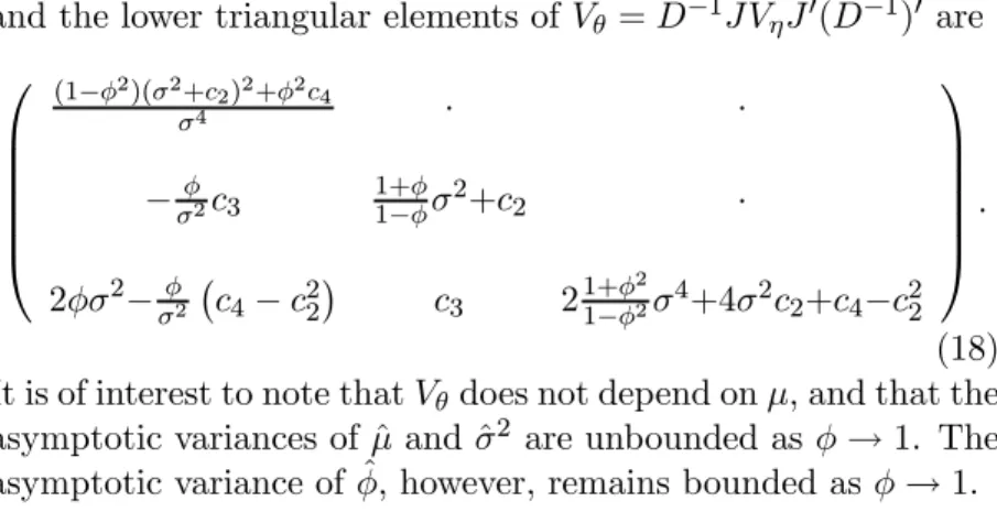
and the lower triangular elements ofY =G31MYM0(G31)0 are 3 E E E E E C (13!2)(2+f2)2+!2f4 4 · · !2f3 1+₁3!!2+f2 · 2!2!2 ¡ f₄f2₂¢ f₃ 21+_13!!₂24+42f₂+f₄f2₂ 4 F F F F F D = (18) It is of interest to note thatYdoes not depend on, and that the

asymptotic variances ofˆ andˆ2 are unbounded as!$ 1. The asymptotic variance of!, however, remains bounded asˆ !$1.

IV. APPLICATION TO THE BRUSSELS ALL SHARES PRICE INDEX

Let uw be the return on the Belgian All Shares Price Index

be-tween successive trading days w1 and w, with w1 ranging from December 31, 1979, to January 15, 2003. The data were taken from Datastream with zero returns removed, as these cor-respond to non-trading weekdays or, almost certainly, to errors. This yielded a total of W = 5627 non-zero returns, and an av-erage yearly (ex-dividend) return equal to ₂₃1₌₀₄P_wuw = 0=0737.

Let u¯ = _W1 PW_w=1uw. Descriptive statistics on the daily returns

uw, the squared de-meaned returns(uwu¯)2 and the log-squared

de-meaned returnslog(uw¯u)2 are given in Table 1.

Table 1: Descriptive statistics

uw (uwu¯)2 log(uwu¯)2

mean 3=02×1034 7=66×1036 11=45

std. deviation 8=75×1033 2=89×1034 2=498

skewness 0=342 19=80 1=109

V. CONCLUSION

Fitting (10) with |w=uw_W1 PWw=1uwgives

log|2w =11=45 + 0=1959(log|2w31+ 11=45)

+p6=239(1(0=1959)2)ˆyw31>

for w= 2> ===> W, where, by construction, _W1₃₁PW_w=2yˆ2_w31 = 1. The indirect estimates of !, and 2 and their standard errors now follow from (16) and (18)7:

ˆ != 0=1959 6=239 6=2394=935 = 0=937> st=err=( ˆ!) = 0=127> ˆ =11=45 + 1=270 =10=18> st=err=(ˆ) = 0=090> ˆ 2 = 6=2394=935 = 1=304> st=err=(ˆ2) = 0=194= The estimate of!, which is close to but smaller than 1, is in line with estimates that have been reported in the literature. The relatively large standard errors of the estimates result from the fact that ! appears to be close to 1, and from the fact that the indirect estimator exploits only the information contained in the mean, variance and first-order autocorrelation of log|2w.

Although SV models are notoriously di!cult to estimate, the use of a judiciously chosen auxiliary model and the application of the method of indirect inference yields an estimator and an associ-ated asymptotic covariance matrix that have simple closed-form expressions. Unfortunately, this comes at a price: the result-ing estimator is very ine!cient. A preliminary comparison with Monte Carlo results by Jacquier, Polson and Rossi (1994) shows that the standard errors of the estimators presented here may be up to 100 times as large as those of the Markov Chain Monte

7_{Standard errors are computed as the square-root of}

W 31 times the

Carlo estimator (though under unfavourable conditions). There-fore, the exploitation of the additional information contained in higher-order autocorrelations oflog|2w, or in moments and

auto-correlations of||w|, will reduce the variance of the estimator con-siderably. It is possible to obtain closed-form expressions both for the optimal weighting matrix of the GMM estimator in this con-text and for its asymptotic covariance matrix. I hope to report on this in the near future.

It would be natural to test, for example, whether the AR(1) specification for the log-volatility is not too restrictive, or whether the normality assumption ofxwin equation (1) is realistic. While

likelihood-based testing methods are presently not feasible, GMM-based methods are relatively straightforward. It is not di!cult to derive moment conditions for an AR(2) specification for log-volatility, hence the standard GMM estimates and standard er-rors yield a test of the AR(1) specification. Furthermore, as-suming that the log-volatility is correctly specified, that kw and

xw are independent processes and that xw is i.i.d., the moment

conditions derived from the expectation and autocorrelations of |_w2 are solely based on the second moment of xw (which equals

one, without loss of generality). Adding moments conditions de-rived from the expectation and autocorrelations of other powers of ||w|, the GMM test for overidentifying restrictions is a test of the normality ofxw.

APPENDIX Calculation of c1, …, c4

For any positive integer q, upon substitutingw={2@2, Z _" 3" ³ log{₂2 ´q 1 I 2h 3{2@2_{g{= 2} Z _" 0 ³ log{₂2 ´q 1 I 2h 3{2@2_g{ = I1 Z _" 0 (logw) q_w31@2_h3w_gw = (q)¡1 2 ¢ ¡1₂¢ >

where (q)_{(}) is the q-th derivative of (}) =}R"

0 w}31h3wgw, the gamma function, and ¡1₂¢ = s. See Abramowitz and Ste-gun (1970) for properties and values of the gamma and related functions. Now, f₁ = Z " 3" (log{2) ³ 1 I 2 ´ h3{2@2g{ = Z _" 3" ³ log{₂2 ´ ³ 1 I 2 ´ h3{2@2g{+ log 2 =#¡1₂¢+ log 2>

where#(}) = _g}g log(}), the digamma function. Forq= 2>3>4, fq= Z " 3" (log{2f₁)q ³ 1 I 2 ´ h3{2@2g{ = Z " 3" ³ log{₂2 #¡1₂¢´q³I1 2 ´ h3{2@2g{ =jq ¡₁ 2 ¢ > where jq(}) = q X l=0 µ q l ¶ (l)(}) (}) (#(})) q3l₌

Some tedious but straightforward algebra shows that j₂(}) =#0(})>

j₃(}) =#00(})>

j₃(}) =#000(}) + 3¡#0(})¢2>

with primes denoting derivatives. Now, #¡1₂¢ = 2 log 2> where = 0=5772 is Euler’s constant, #0¡1₂¢ = ₂2, #00¡1₂¢ =

14(3), where (3) = 1=202 is the value of the Riemann zeta function at 3, and#000¡1₂¢=4. It follows that

f1 =log 2=1=270> f2 = 1₂2 = 4=935>

and

f₄ = 7₄4 = 170=5=

Calculation of Vj

The elements ofˆare the sample mean, variance and first-order autocovariance oflog|w2. Thus, the asymptotic covariance matrix

is Y = lim W<"Var[ s W(ˆ)] = " X m=3" Cov(w> w3m)> where w= 3 C _}}2w w }w}w31 4 D and }w= log|2w f1=

Write }w as nw +zw, where nw = kw and zw = logx2w

f₁. Now, zw and nw have zero mean and are independent, and

we have that Cov(nw> nw3l) = !|l|2, Cov(nwnw3l> nw3m) = 0, and Cov(nwnw3l> nw3mnw3o) = (!|m|+|l3o|+!|o|+|l3m|)4 for any integers

l, m and o. Using these properties, the elements of Y are found

as Y(1>1) = " X m=3" Cov(nw+zw> nw3m+zw3m) = " X m=3" {Cov(nw> nw3m) + Cov(zw> zw3m)}= 1 +! 1! 2_+f 2>

Y(2>2) = " X m=3" Cov£(nw+zw)2>(nw3m+zw3m)2 ¤ = " X m=3" © Cov(n2w> n2w3m) + 4 Cov(nwzw> nw3mzw3m) + Cov(z2w> zw3m2 ) ª = 21 +! 2 1!2 4_{+ 4f} 22+f4f22> Y(3>3) = " X m=3" Cov[(nw+zw)(nw31+zw31)> (nw3m +zw3m)(nw3m31+zw3m31)] = " X m=3" {Cov(nwnw31> nw3mnw3m31) + Cov(nwzw31> nw3mzw3m31) + Cov(nwzw31> zw3mnw3m31) + Cov(zwnw31> nw3mzw3m31) + Cov(zwnw31> zw3mnw3m31) + Cov(zwzw31> zw3mzw3m31)} = µ 1 +!2+ 4 ! 2 1!2 ¶ 4+ 2f₂(1 +!2)2+f2₂> Y(2>1) = " X m=3" Cov[(nw+zw)2> nw3m+zw3m] = " X m=3" Cov(zw2> zw3m) =f3> Y(3>1) = " X m=3" Cov [(nw+zw)(nw31+zw31)> nw3m +zw3m] = 0>

Y(3>2) = " X m=3" Cov£(nw+zw)(nw31+zw31)>(nw3m +zw3m)2 ¤ = " X m=3" © Cov(nwnw31> nw3m2 ) + 2 Cov(nwzw31> nw3mzw3m) +2 Cov(nw31zw> nw3mzw3m)} = 2! µ 1 +1 +! 2 1!2 ¶ 4+ 4f2!2= REFERENCES

Abramowitz, M. and I.A. Stegun, 1970, Handbook of Mathematical Functions, (Dover Publications, New York).

Andersen, T.G., H.-J. Chung and B.E. Sørensen, 1999, Efficient Method of Moments Esti-mation of a Stochastic Volatility Model: a Monte Carlo Study, Journal of Econometrics 91, 61-87.

Andersen, T.G. and B.E. Sørensen, 1996, GMM Estimation of a Stochastic Volatility Model: a Monte Carlo Study, Journal of Business & Economic Statistics14, 328-352.

Andersen, T.G. and B.E. Sørensen, 1997, GMM and QML Asymptotic Standard Deviations in Stochastic Volatility Models: Comments on Ruiz (1994), Journal of Econometrics76, 397-403.

Bollerslev, T., 1986, Generalized Autoregressive Conditional Heteroscedasticity, Journal of Econometrics31, 307-327.

Chib, S., F. Nardari and N. Shephard, 2002, Markov Chain Monte Carlo Methods for Sto-chastic Volatility Models, Journal of Econometrics108, 281-316.

Clark, P.K., 1973, A Subordinated Stochastic Process Model with Finite Variance for Spec-ulative Prices, Econometrica41, 135-155.

Danielsson, J., 1994, Stochastic Volatility in Asset Prices: Estimation with Simulated Max-imum Likelihood, Journal of Econometrics54, 375-400.

Danielsson, J. and J.F. Richard, 1993, Accelerated Gaussian Importance Sampler with Application to Dynamic Latent Variable Models, Journal of Applied Econometrics8, Suppl., S153-S173.

Duffie, D. and K.J. Singleton, 1993, Simulated Moments Estimation of Markov Models of Asset Prices, Econometrica, 61, 929-952.

Engle, R.F., 1982, Autoregressive Conditional Heteroscedasticity with Estimates of the Variance of United-Kingdom Inflation, Econometrica50, 987-1007.

Fridman, M. and L. Harris, 1998, A Maximum Likelihood Approach for Non-Gaussian Sto-chastic Volatility Models, Journal of Business & Economic Statistics16, 284-291. Gallant, A.R., D.A. Hsieh and G.E. Tauchen, 1997, Estimation of Stochastic Volatility

Models with Diagnostics, Journal of Econometrics81, 159-192.

Gallant, A.R. and G.E. Tauchen, 1996, Which Moments to Match? Econometric Theory 12, 657-681.

Gouriéroux, C., A Monfort and E. Renault, 1993, Indirect Inference, Journal of Applied Econometrics8, S85-S118.

Harvey, A.C, E. Ruiz and N. Shephard, 1994, Multivariate Stochastic Volatility Models, Review of Economic Studies61, 247-264.

Hull, J. and A. White, 1987, The Pricing of Options on Assets with Stochastic Volatilities, Journal of Finance17, 281-300.

Jacquier, E., N.G. Polson and P.E. Rossi, 1994, Bayesian Analysis of Stochastic Volatility Models, Journal of Business & Economic Statistics12, 69-87.

Kim, S., N.G. Shephard and S. Chib, 1998, Stochastic Volatility: Optimal Likelihood Infer-ence and Comparison with ARCH Models, Review of Economic Studies45, 361-393. Melino, A. and S.M. Turnbull, 1990, Pricing Foreign Currency Options with Stochastic

Volatility, Journal of Econometrics45, 239-265.

Monfardini, C., 1998, Estimating Stochastic Volatility Models through Indirect Inference, Econometrics Journal1, C113-C128.

Nelson, D.B., 1988, Time Series Behavior of Stock Market Volatility and Returns, Ph.D. dissertation, (MIT).

Nelson, D.B., 1991, Conditional Heteroskedasticity in Asset Returns: a New Approach, Econometrica59, 347-370.

Ruiz, E., 1994, Quasi-Maximum Likelihood Estimation of Stochastic Volatility Models, Journal of Econometrics63, 289-306.

Sandmann, G. and S.J. Koopman, 1998, Estimation of Stochastic Volatility Models via Monte Carlo Maximum Likelihood, Journal of Econometrics87, 271-301.

Tauchen, G.E. and M. Pitts, 1983, The Price Variability-Volume Relationship on Specula-tive Markets, Econometrica51, 484-505.