Estimation of the current population total for a four-phase sampling design

(1)

Estimation of the current population total

for a four-phase sampling design

Viktoras Chadyšas, Danut˙e Krapavickait˙e

Vilnius Gediminas Technical University, Saul˙etekio ave. 11, LT-10283 Vilnius, Lithuania [email protected]; [email protected]

Received:October 1, 2014 / Revised:September 1, 2015 / Published online:December 30, 2015 Abstract.The combined ratio-type estimators of the finite population total and their variances in the case of sample rotation for two-phase and four-phase sampling schemes are constructed in the paper. Combined estimators of the finite population total without and with the use of auxiliary information known from the previous survey are built. Two types of sampling design are used for sample selection in each of the phases: simple random sampling without replacement and successive sampling without replacement with probabilities proportional to size. A simulation study, based on the real data, is performed, and the accuracy of the estimators proposed is compared.

Keywords:sample rotation, successive sampling, ratio estimator, composite estimator.

1 Introduction

A sample survey when information is collected regularly on the same population in sub-sequent time periods with the partial replacement of the sample is studied. Such repetitive surveys (consecutive measurements of the same population) are used in social studies, of-ficial statistics, forestry, medicine etc. The Labour Force Survey (LFS) provides estimates of the number of employed and unemployed individuals for each quarter of the year. Repeated sampling from a finite population (or sample rotation) is a sampling procedure, which is usually used for this survey.

Let us denote a finite household population _U = {1, . . . , i, . . . , N}of sizeN. For each household, the number of its members is denoted bymi,i= 1,2, . . . , N. The sum of household members is obtained byM = PN_i₌₁mi. Let us suppose that the survey variableymeans the number of employed (or unemployed) individuals in each household. The valuesyiof the variable belong to the set of integers{0,1, . . . , mi}. The parameter of interest is the total of the number of employed (or unemployed) individuals

ty = N

X

i=1

(2)

The previous survey data can be used as auxiliary information for the estimation of the population total in order to reduce the variance of the estimator. The efficiency of ratio estimators in the case of any sampling design is discussed in Särndal et al. [21]. Combined estimators of the finite population total without and with the use of auxiliary information known from the previous survey are constructed.

Sample rotation and two-phase sampling (double sampling) are similar procedures. Sample rotation means that a sample of the current occasion consists of a union of sub-samples: one of them is matched with the elements of previous occasions, and the other one is a new one and unmatched with the previously studied elements. A sample under a two-phase sampling design is matched with the first-phase sample.

In this paper, the construction of the combined estimator of the finite population total and its variance in the case of sample rotation is analyzed for two-phase and four-phase sampling schemes.

If the auxiliary variable is well-correlated with the study variable, then it is possible to obtain more accurate estimates of the parameter. A two-phase sampling design and estimators of the total with the use of auxiliary information are given in Särndal et al. [21]. They are applied here to the Lithuanian LFS data in the case of a simple random sample of individuals, and the current paper is a further development of [7].

The estimators for a total in the case of the three-phase sampling design are presented in Fuller [9] and Singh [22]. Jeyaratnam et al. [13] studied multiphase sampling for the stratification and efficient allocation of the sample size. Many various problems are being solved for two occasions sample data. One of them is the optimal choice of the second-occasion sampling design in order to minimize the variance of the estimator (Arnab, [3]). Hamad et al. [10] uses two auxiliary variables for the estimator of the total in a two-phase sampling design. Subsampling of nonrespondents and corresponding estimators is also a case of estimation under a two-phase sampling design (Okafor and Lee, [16]), under a three-phase sampling design (Hidiriglou and Estevao [11]). Artes and Garcia [4] studied the estimators of the ratio under sampling on two occasions with partial replacement of the elements. Close attention is paid to variance estimation for the estimator of change in the finite population parameter in repeated surveys. There are many studies on this topic, for example, Berger [5], Andersson [2], and Qualité [17]. Fattorini et al. [8] studied a special three-phase sampling strategy for the estimation of forest biomass.

Combined estimators of the population total are obtained taking a linear combination of ratio estimators using theπ∗_{estimators idea (Särndal et al., [21]) for a multi-phase} sampling design and the Horvitz–Thompson estimator (Horvitz and Thompson, [12]) or the ratio estimator. Two types of sampling design are used here for sample selection in each of the phases: simple random sampling without replacement and a successive sampling (unequal probability sampling without replacement) procedure proposed by Rosén [18]. The second-order inclusion probabilities for a successive sampling design are approximated by corresponding probabilities for conditional Poisson sampling. The results of Aires [1] and Bondesson et al. [6] are used for this. Then the inclusion prob-abilities obtained are used to calculate the estimates of the proposed estimators of the totals and their variance estimates. A simulation study, based on the real population data, is performed, and the estimators proposed are compared.

(3)

2 Sample rotation and sample selection

The LFS at Statistics Lithuania is conducted continuously with a quarterly selected sam-ple. All members of a household are included in the sample for two subsequent quarters, excluded from the sample for the next two quarters, and included once more in the sample for two other quarters. It means that one-fourth of the sample of the previous quarter is replaced by the new one each quarter of the year as shown in Fig. 1.

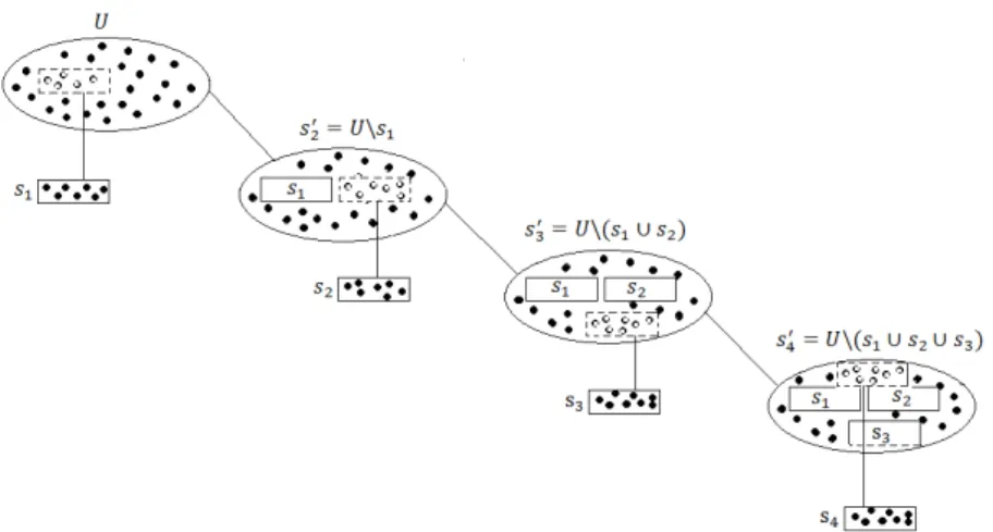
The sample selection procedure is performed as shown in Fig. 2.

It is seen in the sample selection scheme, presented in Fig. 2, that the whole samples

consists of a union of four subsamples:s1,s2,s3ands4. The subsamples selected at each of the phases are expressed:

s1:U →s1;

s2:U →s02=U \s1→s2, two phases;

s3:U →s02=U \s1→s30 =U \(s1∪s2)→s3, three phases;

s4:U →s02=U \s1→s03=U \(s1∪s2)

→s04=U \(s1∪s2∪s3)→s4, four phases.

The estimators under the sampling scheme described will be discussed further.

Figure 1.Sample rotation scheme of the Labour Force Survey.

(4)

3 Simple estimators of the population total

We are interested in the estimation of the population totalty = P_i∈Uyi for a study variabley. Firstly, we construct four separate design-based estimators of the total using data of the sampless1,s2,s3 ands4, respectively. Secondly, we propose a combined estimator of the total using sample rotation schemes in Section 4.

Step 1. The samples1is selected from the finite population:U →s1. The corresponding first- and second-order inclusion probabilities for elements of the samples1are denoted respectively:

π1i=P(i∈s1); π1ij=P(i∈s1, j∈s1), π1ii =π1i.

An unbiased design-based Narain [15] and Horvitz–Thompson [12] estimator of the population total is used:

ˆ tHT 1y = X i∈s1 yi π1i . (2)

The variance of the estimatorˆtHT

1y and its unbiased estimator is Var ˆtHT 1y =X i∈U X j∈U (π1ij−π1iπ1j) yi π1i yj π1j , (3) d Var ˆtHT 1y =X i∈s1 X j∈s1 1₋π1iπ1j π1ij _y i π1i yj π1j . (4)

The values of the study variableyin the previous survey can be used as auxiliary infor-mation. Let us denote the study variable of the previous survey (₋1wave) byxwith the valuesxiand the same variable on the current0wave byywith the valuesyi,i∈s1. We can form the ratio estimatortˆrat

1y of the population totaltyby ˆ trat 1y =t (−1) 1x ˆ t1y ˆ t1x =t(1−x1)r,ˆ rˆ= ˆ t1y ˆ t1x , (5) We use here tˆ1y = ˆt1HTy , tˆ1x = ˆt1HTx , t (−1) 1x = P

i∈Uxi. Some other approximately unbiased estimatorstˆ1y,ˆt1xwill be also used in this situation further. The estimatorˆt1raty is nonlinear. Its approximate variance based on a Taylor linearization of the estimator is expressed as: AVar ˆtrat 1y =X i∈U X j∈U (π1ij−π1iπ1j) yi−rxi π1i yj−rxj π1j (6)

withr=Pi∈Uyi/Pi∈Uxi. The varianceAVar(ˆt1raty)is estimated by

d Var ˆtrat 1y =X i∈s1 X j∈s1 1₋π1iπ1j π1ij _y i−rxˆ i π1i yj−rxˆ j π1j , (7) usingˆrgiven in (5).

(5)

Step 2. The samples2is obtained in two-phase sampling:U →s02=U \s1→s2. The corresponding first- and second-order unconditional and conditional element inclusion probabilities for sampless0

2(first phase) ands2(second phase) are, respectively,

π02ij=P(i∈s 0 2, j∈s 0 2) (8) = 1₋P(i_∈s1, j∈s1)−P(i∈s1, j /∈s1)−P(i /∈s1, j∈s1), π20i=P(i∈s 0 2) =P(i /∈s1) = 1−P(i∈s1), π2i|s0 2=P(i∈s2|s 0 2), π2ij|s0 2=P(i∈s2, j∈s2|s 0 2).

Under a two-phase sampling design, using theπ∗_{estimator defined in [21, Sect. 9.2],} the population totaltyis unbiasedly estimated by

ˆ t(2)2y = X i∈s2 yi π0 2iπ2i|s0 2 . (9)

In the case of two-phase sampling, the variance of the estimatorˆt(2)2y may be expressed by conditional and unconditional variances and expectations:

Var ˆt(2)2y = VarE ˆt(2)2y s02 +E Var ˆt(2)2y s02 = Var ˆt(1)2y +EVar ˆt(2)2y s02 , (10) ˆ t(1)2y = X i∈s0 2 yk π0 2i = X i∈U \s1 yk π0 2i or Var ˆt(2)2y =X i∈U X j∈U (π20ij−π 0 2iπ 0 2j) yi π0 2i yj π0 2j +E X i,j∈s0 2 (π2ij|s0 2−π2i|s02π2j|s02) yi π0 2iπ2i|s0 2 yj π0 2jπ2j|s0 2 . (11)

The varianceVar(ˆt(2)2y)is estimated unbiasedly by

The values of the study variableyin the previous survey (₋3wave) can be used as auxiliary information. Let us denote the study variable of the previous survey byxwith

(6)

the valuesxiand the same variable on the current wave byywith the valuesyi,i ∈s2. We can form a ratio estimatorˆtrat

2y of the population totaltyby

ˆ trat 2y =t (−3) 2x rˆ2, rˆ2= ˆ t(2)2y ˆ t(2)2x , ˆt(2)2x = X i∈s2 xi π0 2iπ2i|s0 2 . (13) Heret(2−x3) = P

i∈Uxiis the total of the variablex, which was a study variableyin the previous survey (₋3wave). The estimatorˆt(2)2y is given by (9).

In the case of two-phase sampling, the varianceVar(ˆtrat

2y)of the estimatorˆt2raty also may be expressed by conditional and unconditional variances and expectations replacing the estimatortˆ(2)2y by the estimatorˆt2raty in (10). Becausetˆ2raty is a nonlinear estimator, the approximate varianceAVar(ˆtrat

2y)ofVar(ˆt2raty)is derived using a linear term of its Taylor expansion, and the approximate variance of the ratio estimatorˆtrat

2y is AVar ˆt2raty =X i∈U X j∈U (π02ij−π02iπ20j) yi π0 2i yj π0 2j +E X i,j∈s0 2 (π2ij|s0 2−π2i|s 0 2π2j|s 0 2) yi−rxi π0 2iπ2i|s0 2 yj−rxj π0 2jπ2j|s0 2 (14)

with the ratiorgiven in (6). As the estimator of the variance will be used

with the estimator of the ratioˆr2given in (13).

Step 3. The samples3is obtained in three-phase sampling: U →s02 =U \s1 →s03 =

U \(s1∪s2)→s3. The corresponding first- and second-order inclusion probabilities for the samples0

2(first phase) were denoted in Step 2, and for sampless03(second phase) and

s3(third phase), the inclusion probabilities are, respectively,

π30i|s0 2=P(i∈s 0 3|s02) and π3i|s0 3 =P(i∈s3|s 0 3).

Under a three-phase sampling design, using theπ∗estimator, the population totalty is unbiasedly estimated by ˆ t(3)3y = X i∈s3 yi π0 2iπ03i|s0 2π3i|s 0 3 . (16)

In this step, the values of the study variableyin the previous survey (₋1wave) can be used as auxiliary information. Let us denote the study variable in the previous survey

(7)

byxwith the valuesxi, and the same variable in the current wave byywith the valuesyi, i∈s3. We can form a ratio estimatorˆtrat

3y of the population totalty:

ˆ trat 3y = ˆt (−1) 3x ˆr3, ˆr3= ˆ t(3)3y ˆ t(3)3x , ˆt(3)3x = X i∈s3 xi π0 2iπ30i|s0 2π3i|s 0 3 . (17) Heret(3−x1)= P

k∈Uxkis the total of the variableyin the−1wave. The estimatorˆt (3) 3y is given in (16).

Step 4. The samples4 is obtained in four-phase sampling: U → s02 =U \s1 →s03 =

U \(s1∪s2)→s04=U \(s1∪s2∪s3)→s4.The corresponding first- and second-order inclusion probabilities for samples0

2(first phase) ands03(second phase) were described in Step 2 and Step 3 previously, and for sampless0

4(third phase) ands4(fourth phase), they are, respectively,

Under four-phase sampling, using theπ∗_{estimator, the population total}_t

yis unbiasedly estimated by ˆ t(4)4y = X i∈s4 yi π0 2iπ03i|s0 2π 0 4i|s0 3π4i|s 0 4 . (18)

More complex estimators are presented further.

4 Combined estimators of the population total

The construction of the combined estimators and their variances of the finite population total (1) in the case of sample rotation for two-phase and four-phase sampling schemes is presented in this section.

1. By a linear combination ofˆt1y andˆt (2)

2y , we obtain the estimator without the use of auxiliary information of the total

ˆ t2= 1 2 ˆt1y+ ˆt (2) 2y . (19)

The expression for the variance of estimator (19) of the total: Var ˆt2 =1 4 Var(ˆt1y) + Var ˆt (2) 2y ) + 2 Cov ˆt1y,ˆt (2) 2y , (20) Cov ˆt1y,ˆt (2) 2y =X k∈U X l∈U l6=k yk π1k yl π0 2l π1k−π (1) 1kl −t2 y,

(8)

π1(1)kl =P(k∈s1, l∈s1). The varianceVar(ˆt2)is estimated unbiasedly by d Var(ˆt2) =1 4 Var(ˆd t1y) +Var ˆd t (2) 2y + 2Cov ˆd t1y,ˆt (2) 2y , (21) d Cov ˆt1y,ˆt (2) 2y = X k∈s1 X l∈s2 yk π1k yl π0 2l π1k−π (1) 1kl π? 2kl −ˆ_t₁_yˆ_t(2) 2y , (22) π? 2kl=P(k∈s1, l∈s02)P(k∈s1, l∈s2|s02) =π1klP(l∈s2|s02).

2. By a linear combination of ˆtrat 1y andˆt

(2)

2y , we obtain the estimator with the use of auxiliary information of the total

ˆ trat 2 = 1 2 ˆt rat 1y + ˆt (2) 2y . (23)

The expression for the variance of estimator (23): Var ˆt2rat =1 4 Var ˆt rat 1y + Var ˆt2(2)y + 2 Cov ˆt1raty,ˆt (2) 2y . (24)

The varianceVar(ˆtrat

2 )is estimated by d Var ˆt2rat =1 4 dVar ˆt rat 1y +Var ˆd t2(2)y + 2Cov ˆd t1raty,tˆ (2) 2y (25) with the covariance estimator

d Cov ˆtrat 1y ,ˆt (2) 2y = X k∈s1 X l∈s2 yk−rxk π1k yk π0 2l π1k−π (1) 1kl π? 2kl . 3. By a linear combination ofˆt1y,tˆ (2) 2y ,tˆ (3) 3y andˆt (4)

4y, we obtain a new estimator without the use of auxiliary information

ˆ t4= 1 4 ˆt1y+ ˆt (2) 2y + ˆt (3) 3y + ˆt (4) 4y . (26)

4. By a linear combination ofˆtrat

1y,ˆt2raty,tˆ3raty andˆt (4)

4y we obtain a new estimator of the total with the use of auxiliary information

ˆ trat 4 = 1 4 ˆt rat 1y + ˆt2raty + ˆt3raty + ˆt (4) 4y . (27)

Further, we are interested in the estimation of the finite population totaltyusing two-phase and four-two-phase sampling schemes, when simple random samples of households without replacement and samples with probabilities proportional to household size with-out replacement are drawn in each of the phases.

(9)

5 Special cases of sampling design

5.1 Simple random sampling of households without replacement 5.1.1 Two-phase sampling scheme

Data for two quarters are used for the estimation of the population totalty. Assume that s1 of size n1 is a simple random sample from the populationU, and its complement

s0

2 =U \s1of sizeN −n1is also a simple random sample from the populationU. s2 of sizen2is a simple random sample froms02. Then the first- and second-order inclusion probabilities to be used for (19) and (23) are calculated as follows:

π1i=P(i∈s1) = n1 N, π1ij=P(i∈s1, j∈s1) = n1 N n1−1 N₋1, i6=j, π0 2i=P(i∈s02) = N₋n1 N , π0 2ij=P(i∈s02, j∈s02) = 1− n1 N n1−1 N−1 −2 n1 N−1 1₋n1 N , i₆=j, π2i|s0 2=P(i∈s2|s 0 2) = n2 N₋n1 , π2ij|s0 2=P(i∈s2, j∈s2|s 0 2) = n2 N−n1 n2−1 N−n1−1 , i₆=j.

In the case of simple random sampling in each of the phases, the estimator of total (19) without the use of auxiliary information can be rewritten as

ˆ t2= 1 2 N n1 X i∈s1 yi+ N n2 X i∈s2 yi . (28)

The variance of the estimatorˆt2of the totaltyis expressed

Var(ˆt2) =1 4 N2 1−n_N1 _s2 1y n1 +N2 1−n_N2 _s2 2y n2 − 2N s2 12y , (29) wheres2 1y=s22y=s212y= (N−1)−1 PN i=1(yi−µy) 2_,_µ y=ty/N. The varianceVar(ˆt2)is estimated unbiasedly by

d Var(ˆt2) =1 4 N2 1−n_N1 _ˆ_s2 1y n1 +N2 1−n_N2 _s_ˆ2 2y n2 − 2Nsˆ212y , (30) where ˆ s2 1y= 1 n1−1 X i∈s1 yi− 1 n1 X j∈s1 yj 2 , sˆ2 2y= 1 n2−1 X i∈s2 yi− 1 n2 X j∈s2 yj 2 ,

(10)

ˆ s212y = 1 n1+n2−1 X i∈s yi− 1 n X j∈s yj 2 , s=s1∪s2.

In the case of simple random sampling, in each of the phases, the estimator of to-tal (23) with the use of auxiliary information can be rewritten as

ˆ trat 2 = 1 2 t(1−x1) P i∈s1yi P i∈s1xi + N n2 X i∈s2 yi . (31)

Heret(1−x1)is the population total of the study variableyin the previous survey (−1wave). An approximate variance of the estimatorˆtrat

2 of the totaltyis expressed AVar(ˆtrat 2 ) = 1 4 N2₁ −n_N1s 2 1y−rx n1 +N2₁ −n_N2s 2 2y n2 − 2N s2 12y−rx,y , (32) where s2 1y−rx= 1 N₋1 N X i=1 (yi−rxi)2, s22y= 1 N₋1 N X i=1 (yi−µy)2, s2 12y−rx,y = 1 N−1 N X i=1 (yi−rxi)(yi−µy), r= PN i=1yi PN i=1xi , µy= ty N.

The varianceVar(ˆtrat

2 )is estimated by d Var ˆtrat 2 = 1 4 N2 1−n_N1 _s_ˆ2 1y−rx n1 +N2 1−n_N2 _ˆ_s2 2y n2 − 2Nsˆ2 12y−rx,y , (33) where ˆ s2 1y−rx= 1 n1−1 X i∈s1 (yi−rxˆ i)2, ˆr= P j∈s1yj P j∈s1xj , ˆ s2 2y = 1 n2−1 X i∈s2 yi− 1 n2 X j∈s2 yj 2 , ˆ s212y−rx,y = 1 n1−1 X i∈s1 (yi−rxˆ i) yi− 1 n1 X j∈s1 yj .

The number of simple random sampling phases is further increased.

5.1.2 Four-phase sampling scheme

Data for four quarters are used for the estimation of the population totalty. Assume that all samples in the selection procedure shown in Fig. 2 are simple random samples:s1of sizen1,s0

2=U \s1of sizeN−n1,s2of sizen2,s30 =U \(s1∪s2)of sizeN−n1−n2,

(11)

first- and second-order inclusion probabilities for sampless1,s0

2ands2are introduced in Subsection 5.1.1. The corresponding first-order inclusion probabilities for sampless0

3,s3,

s0

4,s4to be used for (26) and (27) are calculated as follows:

Now, in the case of simple random sampling, in each of the phases, estimator (26) without the use of auxiliary information of the total can be rewritten as

ˆ t4= 1 4 _N n1 X i∈s1 yi+ N n2 X i∈s2 yi+ N n3 X i∈s3 yi+ N n4 X i∈s4 yi . (34)

In the case of simple random sampling, in each of the phases, estimator (27) with the use of auxiliary information of the total can be rewritten as

ˆ trat 4 = 1 4 t(1−x1) P i∈s1yi P i∈s1xi +t(2−x3) P i∈s2yi P i∈s2xi +t(3−x1) P i∈s3yi P i∈s3xi + N n4 X i∈s4 yi . (35)

Remark 1. The totalst(x−1),t(₂−_x3),t(₃−_x1)in (31), (35) cannot be known in a real survey, because the values of the study variable in all waves are known only for sample data. Therefore, we suggest replacing them by the estimates oftyobtained for the correspond-ing wave uscorrespond-ing the whole sample consistcorrespond-ing of four rotation parts, and to consider them further as fixed.

5.2 Unequal probability sampling of households without replacement with proba-bilities proportional to their size (successive sampling)

The selection of households through individuals is taken as an example of an unequal probability sampling design, which is used for the Lithuanian LFS. An individual is selected from a list with equal selection probabilities, and his/her household is included in the sample. Individual selection is repeated. If the household selected is already in the sample, this selection step is ignored. Otherwise, the household is included in the sample. The process is continued until the predetermined numbernof different households is se-lected. This household selection scheme is studied by Rosén [20] and is called successive sampling design. The larger the household, the higher its probability to be selected for the sample, because any of its members can be selected from the list of individuals.

(12)

5.2.1 Order sampling designs

The order sampling design [18] is defined as follows. To each population elementi_{∈ U}, a probability distributionFi is assigned,i = 1,2, . . . , N. Independent ranking random variablesQ1, Q2, . . . , QN with distributionsF1, F2, . . . , FN are realized. The elements with thensmallestQvalues constitute a sample. The distributionsF1, F2, . . . , FN are called ranking distributions.

Let us consider ranking distributions Fi(u) = H(u;λi) with a shape distribution functionH(u), concentrated on a positive half-line, and real constantsλi > 0, called intensities, desired or target inclusion probabilities,i = 1,2, . . . , N. The class of order sampling designs includes successive and Pareto sampling designs.

Successive sampling designhas an exponential shape distribution function H(u) = 1₋e−u_,₀

6u <_∞. The ranking variables are

Qi=

ln(1−Ui) ln(1₋λi)

, i∈ U, (36)

with the values of the random variablesUidistributed uniformly on[0,1].

ThePareto sampling designhas a Pareto shape distribution functionH(u) =u/(1+u), 06u <_∞. The ranking variables are

Qi=

Ui(1−λi) λi(1−Ui)

, i_{∈ U},

with the values of the random variablesUidistributed uniformly on[0,1].

For these sampling designs, the exact inclusion probabilities are approximately equal to the desired inclusion probabilitiesλi. According to Rosén [19], the inclusion prob-abilities for order sampling designs are asymptotically equal to the desired inclusion probabilitiesλi.

In our case, mi is the number of household members,M = P N

i=1mi is the total number of individuals, and we chooseλi=nmi/M. We obtain that with such a selection of desired inclusion probabilities, the class of order sampling designs intersects with the class of sampling designs with inclusion probabilities approximately proportional to the size measure (PPS).

Theconditional Poisson samplingscheme (CP) is defined as follows: each unit in the population is selected with a prescribed probabilitypi,pi > 0, andP

N

i=1pi = n, but only the samples of the desired sizenare accepted. The inclusion probabilities for the CP sample will not be exactly equal topi, but only approximately.

Expressions for the second-order inclusion probabilitiesπ1ijin the case of order sam-pling design are presented in Aires [1], but they are too complex, and their computation is time-consuming.

According to Bondesson et al. [6, p. 700], Pareto and CP sampling designs are close forpi =λi, and inclusion probabilities of all orders for Pareto sampling design may be approximated by the corresponding ones for the CP design. Relying on the approximate equality of the first-order inclusion probabilities, we will approximate the second-order

(13)

inclusion probabilities for a successive design with the second-order inclusion probabili-ties for the CP design.

5.2.2 Two-phase sampling scheme

Data for two quarters are used for the estimation of the population totalty. Assume that a samples1of sizen1, a samples02 = U \s1 of sizeN −n1, and a sample s2of size

n2are drawn according to the successive sampling design introduced by Rosén [18]. The first-phase household target inclusion probability in the samples1 is defined asλi = n1mi/M,i∈s1. The second-phase household target inclusion probability in the sample s2is defined asλ2i =n2mi/Pj∈s0

2mj,i∈s

0 2.

The first-order inclusion probabilities to be used for the estimation of the total ty in (19) and (23) are expressed approximately as follows:

π1i=P(i∈s1)≈λi= n1mi M , π 0 2i=P(i∈s02)≈λ02i= M₋n1mi M , π2i|s0 2 =P(i∈s2|s 0 2)≈λ2i= n2mi M2 , M2= X j∈s0 2 mj. The estimatorsˆt1y = ˆtλ1y = P i∈s1yi/λi,ˆt1x= ˆt λ 1x= P

i∈s1xi/λiare used in (19), (5)

and (23).

For the estimators of variances (21), (25), the second-order inclusion probabilities for a successive sampling design are needed. Second-order inclusion probabilities for CP samplingπˇ1ij, presented by Aires [1], are

ˇ π1ij = 1 γ1i−γ1j (γ1iˇπ1j−γ1jˇπ1i) forγ1i6=γ1j, (37) ˇ π1ij = 1 k1i (n1−1)ˇπ1i− X j:γ1j6=γ1i ˇ π1ij forγ1i=γ1j, (38)

i, j _{∈ U}, i ₆= j. Hereγ1i = p1i/(1−p1i), and k1i is the number of elements with j_{∈ U},j ₆= i, such thatγ1i = γ1j; the probabilityp1i is a selection probability of the elementifor a CP sampling design,i_{∈ U}. Supposeπˇ1iare given inclusion probabilities to the CP design equal toλi. Keeping them as known, we use the approximation result of Bondesson et al. [6, p. 705] to expressp1ithrough these inclusion probabilities:

γ1i= p1i 1₋p1i ∝ ˇ π1i 1₋πˇ1i exp 1/2−πˇ1i d , d= N X i=1 ˇ π1i(1−πˇ1i).

Inserting theγ1i obtained into (37), we find second-order inclusion probabilities to the CP designπˇ1ij.

ApproximatingP(i∈s1, j∈s1)in (8) byπˇ1ij, we obtain the second-order inclusion probabilities for the samples02, and keepingπ2i|s0

(14)

Herek2iis the number of elementsj6=isuch thatγ2i=γ2jand γ2i= λ2i 1₋λ2i exp ₁_/₂ −λ2i d , d=X i∈s0 2 λ2i(1−λ2i). We haveπˇ2ii|s0 2= ˇπ2i|s 0 2in the case ofi=j.

We remind that the second-order inclusion probabilities for a successive sampling design are approximated by the corresponding probabilities for the CP design.

After replacing theπvalues in (4), (7) and (12) with the corresponding approximate values presented in this section we estimate the variances of the estimatorstˆ2andtˆ2ratof the totaltyin (21) and (25) respectively with

d Cov ˆt1y,ˆt (2) 2y = M 2 n1n2 M₋X i∈s1 mi X k∈s1 X l∈s2 yk mk yl ml 1 M−n1ml − ˆ t1ytˆ (2) 2y , (39) d Cov ˆt1raty,ˆt (2) 2y = M 2 n1n2 M−X i∈s1 mi X k∈s1 X l∈s2 yk−brxk mk yl ml 1 M−n1ml , (40) ˆ r= ˆt1y ˆ t1x , ˆt1y= ˆtλ1y= X i∈s1 yi λi ∼ X i∈s1 yi π1i , tˆ1x= ˆtλ1x= X i∈s1 xi λi ∼ X i∈s1 xi π1i .

The number of unequal probability sampling phases is further increased.

5.2.3 Four-phase sampling scheme

Data for four quarters are used for the estimation of the population totalty. Assume that all samples in the selection procedure shown in Fig. 2 are drawn according to a successive sampling design: s1 of sizen1,s02 =U \s1is of sizeN −n1,s2 is of sizen2,s03 =

U \(s1∪s2)of sizeN−n1−n2,s3is of sizen3,s04 =U \(s1∪s2∪s3)is of size

N−n1−n2−n3ands4is of sizen4. The first- and second-order inclusion probabilities for sampless1,s0

2 ands2are introduced in Subsection 5.2.2. The corresponding first-order inclusion probabilities for samples s03, s3, s04, s4 for the sampling design under

(15)

Second-order inclusion probabilities for a four-phase sampling design are not pre-sented here. Only the empirical variance of the estimates in the case of a four-phase sampling scheme is used in the simulation study.

6 Simulation study

In this section, we present a simulation study for the comparison of the performance of several estimators of the total using data of two and four quarters, with simple random sampling (SRS) and sampling with probability proportional to size (PPS) (successive order sampling) of households without replacement in each of the phases.

We study the real LFS data of Statistics Lithuania. The study population consists of

N = 500households. The variables of interest, y andx, are the number of employed (or unemployed) individuals in the population of households in the current and previous waves. The population totalst(1−x1),t

(−3) 2x ,t

(−1)

3x are available and are used for estimators (23), (27). The correlation coefficient between the variablesxandy in the household population for the number of employed individuals of interest isρ(x, y) = 0.95. It means a strong linear relationship. For the number of unemployed individuals of interest, the correlation coefficient isρ(x, y) = 0.80.

For the two-phase sampling scheme,B = 500sampless1ands2of sizen1 =n2 = 100 (n = n1 +n2 = 200) are selected by simple random sampling and successive sampling.

For the four-phase sampling scheme, sampless1,s2,s3ands4of sizen1 = n2 =

n3=n4= 50(n=n1+n2+n3+n4= 200) are selected by simple random sampling and successive sampling.

For each of the estimatorsˆt2,ˆt2rat,tˆ4andˆt4rat, we have calculated the estimates of the population totalty of the study variabley. For all estimatorsθˆ = ˆt2,tˆ2rat,ˆt4,ˆt4rat, the averages of the estimates, the averages of the variance estimates and the empirical variances of the estimates

¯ˆ θ= 1 B B X i=1 ˆ θi, Var(ˆd θ) = 1 B B X i=1 d Var(ˆθi), Varemp(ˆθ) = 1 B B X i=1 (ˆθi−θ¯ˆ)2

(16)

Table 1.Average of variance estimates and empirical variances for each part of the combined estimator in two-phase successive sampling.

Estimator Number of employed Number of unemployed Empirical Aver. estimate Empirical Aver. estimate

ˆ tHT 1y 1st part 1 177 1 331 209 197 ˆ trat 1y 1st part rat. 208 180 120 83 ˆ t₂(2)_y 2nd part 1 320 1 296 195 198 ˆ t2 Combined 490 657 74 99 ˆ trat 2 Comb. rat. 363 369 76 70

are calculated. The results of the simulation are presented in Table 1. They illustrate the averages of the estimates of variances and empirical variances for each part of the combined estimatorsˆt2 andˆt2rat, when samples are drawn according to the successive sampling design in each phase.

The combined estimator has a smaller variance than any of its parts first of all because of a higher sample size used to calculate it. Using the ratio estimator, the empirical variance of the estimator of the total decreases for the number of employed individuals and has small effect on the estimates of the number of unemployed individuals.

In almost all cases, the calculated averages of the estimates of variances are close to the empirical variances of the estimates for all parts of combined estimatorsˆt2 andˆt2rat using a two-phase sampling design. It shows that the expression of variance of a combined estimator of the total obtained for two-phase successive sampling is accurate enough, and the inclusion probabilities for a successive sampling design can be approximated by the corresponding probabilities of unequal probability without replacement conditional Poisson sampling design to calculate estimates of the proposed estimators of the totals and their variance estimators.

The box-plot diagrams of the estimates of the number of employed and unemployed individuals in the household population using the proposed estimatorsˆt2, ˆtrat

2 , ˆt4 and ˆ

trat

4 are presented in Figs. 3 and 4. Simple random samples (SRS) and successive samples with probabilities proportional to the household size (PPS) are drawn in each of the phases using two-phase and four-phase sampling schemes.

The estimates of the number of employed individuals have a lower variance using the PPS sampling design, compared to the SRS sampling design. The estimates calculated for the combined ratio estimator of the total for the four-phase sampling scheme has lower variance than the estimates calculated for the combined estimator of the total without the use of auxiliary information. The estimates with the lowest variance are obtained by the combined ratio estimator of the total for four-phase sampling with PPS sampling in each of the phases. The variances of the estimates of the number of unemployed individuals do not differ much.

The box-plot diagrams of the variance estimates of the number of employed and unemployed persons in the household population using all the estimators obtainedtˆ2, ˆ

trat

2 , ˆt4 and ˆt4rat are presented in Fig. 5. The estimates of the variances of estimators of the number of employed individuals using the two-phase sampling scheme with PPS in each of the phases are lower than those obtained with the SRS sampling design. The

(17)

Estimation of the current population total 257

probabilities for a successive sampling design can be approximated by

the corresponding probabilities of unequal probability without replacement

conditional Poisson sampling design to calculate estimates of the proposed

estimators of the totals and their variance estimators.

The box-plot diagrams of the estimates of the number of employed and

unemployed individuals in the household population using the proposed

estimators ˆ

t

2

, ˆ

t

rat2

, ˆ

t

4

and ˆ

t

rat4

are presented in Fig. 3 and Fig. 4. Simple

random samples (SRS) and successive samples with probabilities

propor-tional to the household size (PPS) are drawn in each of the phases using

two-phase and four-phase sampling schemes.

Figure 3: Estimates of the number of employed individuals

Figure 4: Estimates of the number of unemployed individuals

The estimates of the number of employed individuals have a lower

variance using the PPS sampling design, compared to the SRS sampling

19

Figure 3.Estimates of the number of employed individuals.

the corresponding probabilities of unequal probability without replacement

conditional Poisson sampling design to calculate estimates of the proposed

estimators of the totals and their variance estimators.

The box-plot diagrams of the estimates of the number of employed and

unemployed individuals in the household population using the proposed

estimators ˆ

t

2

, ˆ

t

rat2

, ˆ

t

4

and ˆ

t

rat4

are presented in Fig. 3 and Fig. 4. Simple

random samples (SRS) and successive samples with probabilities

propor-tional to the household size (PPS) are drawn in each of the phases using

two-phase and four-phase sampling schemes.

Figure 3: Estimates of the number of employed individuals

Figure 4: Estimates of the number of unemployed individuals

The estimates of the number of employed individuals have a lower

variance using the PPS sampling design, compared to the SRS sampling

19

Figure 4.Estimates of the number of unemployed individuals.

design. The estimates calculated for the combined ratio estimator of the total for the four-phase sampling scheme has lower variance than the esti-mates calculated for the combined estimator of the total without the use of auxiliary information. The estimates with the lowest variance are obtained by the combined ratio estimator of the total for four-phase sampling with PPS sampling in each of the phases. The variances of the estimates of the number of unemployed individuals do not differ much.

The box-plot diagrams of the variance estimates of the number of em-ployed and unemem-ployed persons in the household population using all the estimators obtained. ˆt2, ˆtrat2 , ˆt4 and ˆtrat4 are presented in Fig. 5.

Figure 5: Estimates of the variances of estimators for the number of employed (left) and unemployed (right) individuals

The estimates of the variances of estimators of the number of employed individuals using the two-phase sampling scheme with PPS in each of the phases are lower than those obtained with the SRS sampling design. The lowest variance has a combined ratio estimator of the total with the use of auxiliary information. The variation of estimates for the variances of estimators of the number of unemployed individuals differs little, and this is because the correlation coefficient between the variables x and y in the household population for the number of unemployed individuals is lower than for the number of employed individuals.

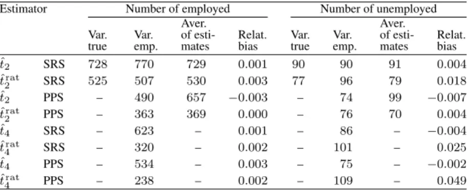
Table 2 illustrates the true variances, averages of the estimates of vari-ances, empirical variances and relative empirical biases:

RB(θb) = 1 ty 1 B B X i=1 (θbi−ty)

of each of the combined estimators obtained before, when SRS and PPS without replacement were drawn in each of the phases.

design. The estimates calculated for the combined ratio estimator of the

total for the four-phase sampling scheme has lower variance than the

esti-mates calculated for the combined estimator of the total without the use of

auxiliary information. The estimates with the lowest variance are obtained

by the combined ratio estimator of the total for four-phase sampling with

PPS sampling in each of the phases. The variances of the estimates of the

number of unemployed individuals do not differ much.

The box-plot diagrams of the variance estimates of the number of

em-ployed and unemem-ployed persons in the household population using all the

estimators obtained. ˆ

t

2

, ˆ

t

rat2

, ˆ

t

4

and ˆ

t

rat4

are presented in Fig. 5.

Figure 5: Estimates of the variances of estimators for the number of

employed (left) and unemployed (right) individuals

The estimates of the variances of estimators of the number of employed

individuals using the two-phase sampling scheme with PPS in each of the

phases are lower than those obtained with the SRS sampling design. The

lowest variance has a combined ratio estimator of the total with the use

of auxiliary information. The variation of estimates for the variances of

estimators of the number of unemployed individuals differs little, and this

is because the correlation coefficient between the variables

x

and

y

in the

household population for the number of unemployed individuals is lower

than for the number of employed individuals.

Table 2 illustrates the true variances, averages of the estimates of

vari-ances, empirical variances and relative empirical biases:

RB

(

θ

b

) =

1 t

y

1 B

B

X

i=1

(

b

θ

i

−

t

y

)

of each of the combined estimators obtained before, when SRS and PPS

without replacement were drawn in each of the phases.

Figure 5. Estimates of the variances of estimators for the number of employed (left) and unemployed (right) individuals

lowest variance has a combined ratio estimator of the total with the use of auxiliary information. The variation of estimates for the variances of estimators of the number of unemployed individuals differs little, and this is because the correlation coefficient between the variablesxandyin the household population for the number of unemployed individuals is lower than for the number of employed individuals.

(18)

Table 2.True variances, empirical variances, averages of variance estimates, and relative biases. Estimator Number of employed Number of unemployed

Aver. Aver.

Var. Var. of esti- Relat. Var. Var. of esti- Relat. true emp. mates bias true emp. mates bias

ˆ t2 SRS 728 770 729 0.001 90 90 91 0.004 ˆ trat 2 SRS 525 507 530 0.003 77 96 79 0.018 ˆ t2 PPS – 490 657 −0.003 – 74 99 −0.007 ˆ trat 2 PPS – 363 369 0.000 – 76 70 0.004 ˆ t4 SRS – 623 – 0.001 – 86 – −0.004 ˆ trat 4 SRS – 320 – 0.002 – 101 – 0.025 ˆ t4 PPS – 534 – 0.003 – 75 – −0.002 ˆ trat 4 PPS – 238 – 0.002 – 109 – 0.049

Table 2 illustrates the true variances, averages of the estimates of variances, empirical variances and relative empirical biases:

RB(ˆθ) = 1 ty 1 B B X i=1 (ˆθi−ty)

of each of the combined estimators obtained before, when SRS and PPS without replace-ment were drawn in each of the phases.

At present, only empirical variances of estimates have been calculated for the four-phase sampling schemes in the case of SRS and successive sampling, in each of the phases. Empirical variances of the estimates of the number of employed persons are lower in the case of a successive sampling design than in the case of SRS. The smallest empirical variance of the estimates of the number of employed individuals has been obtained for the combined ratio estimator when the four-phase sampling has been used. Relative biases for the estimator of employed individuals are insignificant. Combined ratio estimators for the number of the unemployed have a high variance and high relative bias in comparison with the estimates without auxiliary information.

Conclusions

The results of the simulation study show that:

• The ratio type combined estimator in a four-phase LFS sampling design has a lower variance for the estimate of the number of employed individuals and a higher variance for the estimates of the number of the unemployed in comparison with the corresponding estimators, which do not use auxiliary data.

• The approximation of the second order inclusion probabilities for a successive sampling with the corresponding probabilities for conditional Poisson sampling may be used to estimate the variances of the estimator in successive sampling.

• The successive sampling design used in the Lithuanian LFS is effective in the estimation of the number of employed individuals and its effectiveness is the same or even worse than for SRS in the estimation of the number of the unemployed.

(19)

7 Discussion

A two-phase sampling design with second-phase stratification by the household size has been used to estimate the number of employed and unemployed individuals in [14]. The simulation results show that the variance for the estimates of the number of employed individuals decreases significantly in comparison with the one-phase sampling design of the same size, and it does not decrease for the estimates of the number of the unemployed. As we see, the result of the [14] study leads to a similar conclusion as in the case of the current paper.

The combined ratio-type estimator may be effectively used in practice for the estima-tion of the number of employed individuals. When using ratio-type estimators, the data of the elements belonging to the current sample and to the sample of the previous wave, the data of the previous wave are needed. In the case of non-availability of the data of the previous wave for some elements, the values of the variables needed have to be imputed. The ratio estimator used here is the simplest way to use auxiliary information at the estimation stage. A regression estimator of the total with the study variable of the previous wave as an auxiliary variable may also be used. A larger number of auxiliary variables from the previous waves and a calibrated estimator of the total instead of a ratio estimator is a possible generalization of the problem.

Acknowledgment. The authors are thankful to three anonymous referees for valuable comments, resulting in a significant improvement of the paper.

References

1. N. Aires, Algorithms to find exact inclusion probabilities for conditional Poisson sampling and Paretoπpssampling designs,Methodol. Comput. Appl. Probab.,1(4):457–469, 1999. 2. A. Andersson, K. Andersson, P. Lundquist, Estimation of change in a rotation panel design,

inBulletin of the International Statistical Institute Proceedings of the 58th World Statistics Congress, Dublin, August 21–26, 2011, ISI, The Hague, 2012, pp. 4520–4525, http:// 2011.isiproceedings.org/papers/950903.pdf.

3. R. Arnab, Sampling on two occasions: Estimator of population total, Survey Methodology,

24(2):185–192, 1998.

4. E. Artes, A. Garcia, Estimation of current population ratio in successive sampling,J. Indian Soc. Agric. Stat.,54(3):342–354, 2001.

5. Y.G. Berger, R. Priam,A simple variance estimator of change for rotating repeated surveys: An application to the EU-SILC household surveys, Southampton Statistical Sciences Research Institute, 2013,http://eprints.soton.ac.uk/347142/.

6. L. Bondesson, I. Traat, A. Lundqvist, Pareto sampling versus Sampford and conditional Poisson sampling,Scand. J. Stat.,33:699–720, 2006.

7. V. Chadyšas, D. Krapavickait˙e, Estimation of employed persons in the case of sample rotation,

(20)

8. L. Fattorini, M. Marcheselli, C. Pisani, A three-phase sampling strategy for large-scale multiresource forest inventories, J. Agric. Biol. Environ. Stat., 11(3):296–316, 2006, doi:10.1198/108571106X130548.

9. W.A. Fuller, Estimation for multiple phase samples, in: R.L. Chambers, J. Skinner (Eds.),

Analysis of Survey Data, John Wiley & Sons, Chichester, 2003, pp. 307–322.

10. N. Hamad, M. Hanif, N. Haider, A regression type estimator with two auxiliary variables for two-phase sampling,Open Journal of Statistics,3:74–78, 2013,http://www.scirp. org/journal/ojs/.

11. M.A. Hidiriglou, V. Estevao, Dealing with nonresponse using follow up, inProceedings of the Joint Statistical Meeting, Montréal, Québec, Canada, August 3–8, 2013, American Statistical Association, 2013, pp. 1478–1489.

12. D.G. Horvitz, D.J. Thompson, A generalization of sampling without replacement from a finite universe,J. Am. Stat. Assoc.,47:663–685, 1952.

13. S. Jeyaratnam, D.C. Bowden, F.A. Graybill, W.E. Frayer, Estimation in multiphase designs for stratification,Forest Sci.,30(2):484–491, 1984.

14. D. Krapavickait˙e, The first phase order sampling for the second phase stratification, in

Proceedings of the 59th World Statistics Congress of the International Statistical Institute, Hong Kong, August 25–30, 2013, ISI, The Hague, 2013, pp. 3714–3719,http://2013. isiproceedings.org/Files/CPS016-P8-S.pdf.

15. R.D. Narain, On sampling without replacement with varying probabilities,J. Indian Soc. Agric. Stat.,3:169–174, 1951.

16. F.C. Okafor, H. Lee, Double sampling for ratio and regression estimation with sub-sampling the non-respondents,Survey Methodology,26(2):183–188, 2000.

17. L. Qualité, Y. Tillé, Variance estimation of changes in repeated surveys and its application to the Swiss survey of value added,Survey Methodology,34(2):173–181, 2008.

18. B. Rosén, On sampling with probability proportional to size, R&D Report 1996:1, Statistics Sweden, 1996.

19. B. Rosén, Orderπps inclusion probabilities are asymptotically correct, R&D Report 2001:2, Statistics Sweden, 2001.

20. B. Rosén, Variance estimation for systematic pps-sampling, R&D Report 1991:15, Statistics Sweden, 1991.

21. C.E. Särndal, B. Swensson, J. Wretman,Model Assisted Survey Sampling, Springler-Verlag, New York, 1992.

22. S. Singh,Advanced Sampling Theory with Applications: How Michael Selected Amy, Vols. 1,2, Kluwer Academic, The Netherlands, 2003.