University of California, Berkeley
U.C. Berkeley Division of Biostatistics Working Paper Series
Year Paper
Optimal Spatial Prediction Using Ensemble
Machine Learning
Molly M. Davies
∗Mark J. van der Laan
†∗University of California, Berkeley Division of Biostatistics, [email protected] †University of California, Berkeley, Division of Biostatistics, [email protected]
This working paper is hosted by The Berkeley Electronic Press (bepress) and may not be commer-cially reproduced without the permission of the copyright holder.
http://biostats.bepress.com/ucbbiostat/paper305 Copyright c2012 by the authors.
Optimal Spatial Prediction Using Ensemble
Machine Learning
Molly M. Davies and Mark J. van der Laan
Abstract
Spatial prediction is an important problem in many scientific disciplines. Su-per Learner is an ensemble prediction approach related to stacked generalization that uses cross-validation to search for the optimal predictor amongst all convex combinations of a heterogeneous candidate set. It has been applied to non-spatial data, where theoretical results demonstrate it will perform asymptotically at least as well as the best candidate under consideration. We review these optimality properties and discuss the assumptions required in order for them to hold for spa-tial prediction problems. We present results of a simulation study confirming Super Learner works well in practice under a variety of sample sizes, sampling designs, and data-generating functions. We also apply Super Learner to a real world dataset.
1. INTRODUCTION
Optimal prediction of a spatially indexed variable is a crucial task in many scientific disci-plines. Numerous algorithmic approaches have been proposed (see Cressie (1993) and Sch-abenberger and Gotway (2005) for reviews), but selecting the best approach for a given data set remains a difficult statistical problem. One particularly challenging aspect of spatial pre-diction is that location is often used as a surrogate for large sets of unmeasured spatially indexed covariates. In such instances, effective prediction algorithms capable of capturing lo-cal variation must make strong, mostly untestable assumptions about the underlying spatial structure of the sampled surface and can be prone to overfitting. Ensemble predictors that combine the output of multiple predictors can be a useful approach in these contexts, allow-ing one to consider multiple aggressive predictors. There have been some recent examples of the use of ensemble approaches in the spatial and spatiotemporal literature. For example, Zaier et al. (2010) used ensembles of artificial neural networks to estimate the ice thickness of lakes and Chen and Wang (2009) used stacked generalization to combine support vec-tor machines classifying land-cover types in hyperspectral imagery. Ensembling techniques have also been used to make spatially indexed risk maps. For example, Rossi et al. (2010) used logistic regression to combine a library of four base learners trained on a subset of the observed data to obtain landslide susceptibility forecasts for the central Umbrian region of Italy. Kleiber et al. (2011) have developed a Bayesian model averaging technique for obtain-ing locally calibrated probabilistic precipitation forecasts by combinobtain-ing output from multiple deterministic models.
The Super Learner prediction algorithm is an ensemble approach that combines a user-supplied library of heterogeneous candidate learners in such a way as to minimize ν-fold cross-validated risk (Polley and van der Laan, 2010). It is a generalization of the stacking algorithm first introduced by Wolpert (1992) within the context of neural networks and later adapted by Breiman (1996) to the context of variable subset regression. LeBlanc and Tibshirani (1996) discuss stacking and its relationship to the model-mix algorithm of Stone
(1974) and the predictive sample-reuse method of Geisser (1975). The library on which Super Learner trains can include parametric and nonparametric models as well as mathematical models and other ensemble learners. These learners are then combined in an optimal way in the sense that the Super Learner predictor will perform asymptotically as well as or better than any single prediction algorithm in the library under consideration. Super Learner has been used successfully in nonspatial prediction (see for example Polley et al. (2011)). In this paper, we review its optimality properties and discuss the assumptions necessary for these optimality properties to hold within the context of spatial prediction. We also present the results of a simulation study, demonstrating that Super Learner works well in practice under a variety of spatial sampling schemes and data-generating distributions. In addition, we apply Super Learner to a real world dataset, predicting water acidity for a set of 112 lakes in the Southeastern United States. We show Super Learner is a practical, data-driven, theoretically supported way to build an optimal spatial prediction algorithm from a large, heterogeneous set of predictors, protecting against both model misspecification and over-fitting.
2. PROBLEM FORMULATION
Consider a random spatial process indexed by location over a fixed, continuous,d-dimensional domain,Y(s) :s∈D⊂Rd .For a particular set of distinct sampling points {S
1, ..., Sn} ⊂
D, We observe{(Si, Yi∗) :i= 1, . . . , n},whereY∗ =Y(Si)+iandirepresents measurement
error for the ith observation. For all i, we assume E[Yi∗|Si =s] = Y(s). Our objective is to
predictY(s0) for unobserved locations s0 ⊂D. Thus, our parameter of interest is the spatial process itself. We do not make any assumptions about the functional form of the spatial process. We do, however, assume that one of the following is true: for all i, either
(1) (Si, Yi∗) are independently and identically distributed (i.i.d.), or
(2) (Si, Yi∗) are independent but not identically distributed, or
Each of these sets of assumptions imply that any measurement error is mean zero conditional onSi, or in the case of fixed design, conditional onS1, . . . ,Sn. It is important to note thatS
could consist of both location and some additional covariatesW, i.e. S= (X,W), where X refers to location. In such cases, it may be that measurement error is mean zero conditional on location and covariates, but not on location alone.
While these are reasonable assumptions for many spatial prediction problems, they are nontrivial and may not always be appropriate. For instance, instrumentation and calibration error within sensor networks can result in spatially structured measurement error that is not mean zero given S1, . . . ,Sn. There has been an effort on the part of researchers to develop
ways to adapt the cross-validation procedure so as to minimize the effects of this kind of measurement error when choosing parameters such as bandwidth in local linear regression or smoothing parameters for splines. Interested readers should consult Opsomer et al. (2001) and Francisco-Fernandez and Opsomer (2005) for overviews.
3. THE SUPER LEARNER ALGORITHM
Suppose we have observed {Oi}ni=1, drawn from the random variable O with true
data-generating distribution P0 ∈ M, where the statistical model M contains all possible data
generating distributions for O. The empirical distribution for our sample is denoted Pn.
Define a parameter Ψ : M → R ≡ {Ψ(P) : P ∈ M} in terms of a risk function R as follows: Ψ(P) = argminψ∈ΨR(ψ, P). In this paper, we will limit our discussion to so-called linear risk functions, where R(ψ, P) = P L(ψ) = R L(ψ)(o)dP(o) for some loss function
L. For a discussion of nonlinear risk functions, see van der Laan and Dudoit (2003). We write our parameter of interest as ψ0 = Ψ(P0) = argminψR(ψ, P0), a function of the true
data generating distributionP0. For many spatial prediction applications, the Mean-Squared
Error (MSE) is an appropriate choice for the risk function R, but this needn’t necessarily be the case.
Define a library of J base learners of the parameter of interest ψ0, denoted {Ψbj : Pn → b
exam-ple, within the context of spatial prediction, a library could consist of various Kriging and smoothing splines algorithms, Bayesian hierarchical models, mathematical models, machine learning algorithms, and other ensemble algorithms. We make a minimal assumption about the size of the library: it must be at most polynomial in sample size. Given this library of base learners, we consider a family of combining algorithms {Ψbα = f({Ψbj : j}, α) : α}
in-dexed by a Euclidean vectorα for some functionf. One possible choice of combining family is the family of linear combinations, Ψbα =
PJ
j=1α(j)Ψbj. If it is known that ψ0 ∈[0,1], one
might instead consider the logistic family, log[Ψbα/(1−Ψbα)] = PJ
j=1α(j) log[Ψbα/(1−Ψbα)].
In either of these families, one can also constrain the values α can take. In this paper, we constrain ourselves to convex combinations, i.e. for all j, α(j)≥0 and P
jα(j) = 1.
Let{Bn}be a collection of length nbinary vectors that define a random partition of the
observed data into a training set{Oi :Bn(i) = 0}and a validation set{Oi :Bn(i) = 1}. The
empirical probability distributions for the training and validation sets are denotedP0
n,Bn and
P1
n,Bn, respectively. The estimated risk of a particular estimator Ψ :b Pn → Ψ(b Pn) obtained
via cross-validation is defined as
EBn h R b ΨPn,0Bn, Pn,1Bn i =EBn h Pn,1BnL b ΨPn,0Bn i =EBn Z LΨb Pn,0Bn , ydPn,1Bn .
Given a particular class of candidate estimators indexed α, the cross-validation selector selects the candidate which minimizes the cross-validated risk under the empirical distribu-tion Pn, denoted αn≡argmin α n EBn h RΨbα Pn,0Bn, Pn,1Bnio.
The Super Learner estimate of ψ0 is denoted Ψbαn(Pn).
3.1 Key Theoretical Results
Super Learner’s aggressive use of cross-validation is informed by a series of theoretical results originally presented in van der Laan and Dudoit (2003) and expanded upon in van der Vaart
et al. (2006). We provide a summary of these results below. For details and proofs, the reader is referred to these papers.
First, we define a benchmark procedure called the oracle selector, which selects the can-didate estimator that minimizes the cross-validated risk under the true data generating dis-tribution P0. We denote the oracle selector for estimators based on cross-validation training
sets of size n(1−p), where pis the proportion of observations in the validation set, as
e αn ≡argmin α n EBn h R b Ψα Pn,0Bn, P0 io .
van der Laan and Dudoit (2003) present an oracle inequality for the cross-validation selector αn in the case of random design regression. Let L(·) be a uniformly bounded loss
function with M1 ≡supψ,O|L(ψ)[O]−L(ψ0)[O]|<∞. Letdn(ψ, ψ0) = P0[L(ψ)−L(ψ0)] be
a loss-function based risk dissimilarity between an arbitrary predictor ψ and the parameter of interest ψ0, where the risk dissimilarity dn(·) is quadratic in the difference between ψ
and ψ0, i.e. P0[L(ψ)−L(ψ0)]2 ≤ M2P0[L(ψ −ψ0)]. Suppose the cross-validation selector
αn defined above is a minimizer over a grid of Kn different α-indexed candidate estimators.
Then for any real-valued δ >0,
E h dn b Ψαn Pn,0Bn, ψ0 i ≤(1 + 2δ)Ehmin α EBndn b Ψα[Pn,0Bn], ψ0 i +C(M1, M2, δ) logKn n , (1)
where C(·) is a constant defined in van der Vaart et al. (2006) (see also Appendix B for a definition within the context of fixed regression). Thus if the proportion of observations in the training set, p, goes to zero asn → ∞, and
1 nlognE h min α EBndn b Ψα Pn,0Bn, ψ0 i n→∞ −−−→0,
it follows thatΨbαn, the estimator selected by the cross-validation selector, is asymptotically
equivalent to the estimator selected by the oracle,Ψb
e
size n(1−p), in the sense that EBn h dΨbαn P0 n,Bn , ψ0 i EBn h dΨb e αn P0 n,Bn , ψ0 i n→∞ −−−→1.
The oracle inequality as presented in equation (1) shows us that if none of the base learners in the library are a correctly specified parametric model and therefore do not con-verge at a parametric rate, the cross-validation selector performs as well in terms of expected risk dissimilarity from the truth as the oracle selector, up to a typically second order term bounded by (logKn)/n. If one of the base learnersis a correctly specified parametric model
and thus achieves a parametric rate of convergence, the cross-validation selector converges (with respect to expected risk dissimilarity) at an almost parametric rate of (logKn)/n.
For the special case where Y∗ = Y and the dimension of S is two, the cross-validation selector performs asymptotically as well as the oracle selector up until a constant factor of (logKn)/n. When Y∗ = Y and the dimension of S is greater than two, the rates of
convergence of the base learners will be n−1/d. This is slower than n−1/2, the rate for a correctly specified parametric model, so the asymptotic equivalence of the cross-validation selector with the oracle selector applies.
The original work of van der Laan and Dudoit (2003) used a random regression formula-tion. Spatial prediction problems where we have assumed either (2) or (3) in section 2 above require a fixed design regression formulation. We provide a proof of the oracle inequality for the fixed design regression case in Appendix B.
The key message is that Super Learner is a data-driven, theoretically supported way to build the best possible prediction algorithm from a large, heterogeneous set of predictors. It will perform asymptotically as well as or better than the best candidate prediction algorithm under consideration. Expanding the search space to include all convex combinations of the candidates can be an important advantage in spatial prediction problems, where location is often used as a surrogate for unmeasured spatially indexed covariates. Super Learner allows
one to consider sufficiently complex, flexible functions while providing protection against overfitting.
4. CROSS-VALIDATION AND SPATIAL DATA
The theoretical results outlined above depend on the training and validation sets being inde-pendent. When this is not the case, there are generally no developed theoretical guarantees of the asymptotic performance of any cross-validation procedure (Arlot and Celisse, 2010). Bernstein’s inequality, which van der Laan and Dudoit (2003) use in developing their proof of the oracle inequality, has been extended to accommodate certain weak dependency struc-tures, so it may be that there are ways to justify certain optimality properties of ν-fold cross-validation in these cases. There have also been some extensions to potentially use-ful fundamental theorems that accommodate other specific dependency structures. Lumley (2005) proved an empirical process limit theorem for sparsely correlated data which can be extended to the multidimensional case. Jiang (2009) provided probability bounds for uniform deviations in data with certain kinds of exponentially decaying one-dimensional dependence, although it is unclear how to extend these results to multidimensional dependency structures where sampling may be irregular. Neither of these extensions is immediately applicable to the general spatial case, where sampling may or may not be regular and the extent of spatial correlation cannot necessarily be assumed to be sparse. There has been some attention in the spatial literature to the use of cross-validation within the context of Kriging and selecting the best estimates for the parameters in a covariance function, most of it urging cautious and exploratory use (Cressie, 1993; Davis, 1987). Todini (2001) has investigated methods to provide accurate estimates of model-based Kriging error when the covariance structure has been selected via leave-one-out cross-validation, although this remains an open problem.
Recall from section 2 above that our parameter of interest is the spatial process Y(s) and we have assumed E[Y∗|S =s] =Y(s). Even if Y(s) is a spatially dependent stochastic process such as a Gaussian random field, the true parameter of interest in most cases is not the full stochastic process, but rather the particular realization from which we have
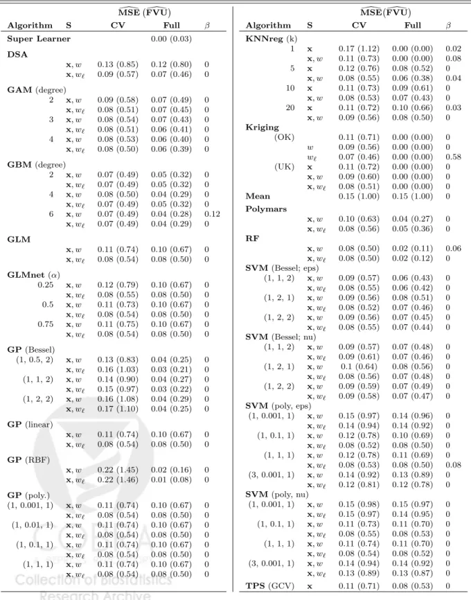
sam-f1 f2 f3 f4 f5 f6 −4 −2 0 2 4
Figure 1: The six spatial processes used in the simulation study. All surfaces were simulated once on the domain [0,1]2. Process values for all surfaces were scaled to [−4,4]⊂R.
pled. Conditioning on this realization removes all randomness associated with the stochastic process, and any remaining randomness comes from the sampling design and measurement error. So long as the data conform to one of the statistical models outlined above in section 2, the optimality properties outlined above will apply.
5. SIMULATION STUDY
We applied the Super Learner prediction algorithm to six data sets with known data gener-ating distributions simulated on a grid of 128×128 = 16,384 points in [0,1]2 ⊂
R2. Each
spatial process was simulated once, hence samples of stochastic processes were taken from a common realization. All simulated processes were scaled to [−4,4] before sampling.
f1(·) is a mean zero stationary GRF with Mat´ern covariance function (Mat´ern, 1986) C(h, θ) = σ2 21−ν Γ(ν) h φ ν Kν h φ +τ2, θ= σ2 = 5, φ= 0.5, ν = 0.5, τ2 = 0,
where h is a distance magnitude between two spatial locations, σ2 is a scaling parameter,
φ >0 is a range parameter influencing the spatial extent of the covariance function andτ2 is
a parameter capturing micro-scale variation and/or measurement error. Kν(·) is a modified
Bessel function of the third order and ν > 0 parametrizes the smoothness of the spatial covariation. Learners were given spatial location as covariates.
f2(·) is a smooth sinusoidal surface used as a test function in both Huang and Chen (2007)
and Gu (2002), f2(s) = 1 + 3 sin (2π[s1 −s2]−π). Learners were given spatial location as
covariates.
f3(·) is a weighted nonlinear function of a spatiotemporal ”cyclone” Gaussian random
field and an exponential decay function of distances to a set of randomly chosen points in [−0.5,1.5]2 ⊂
R2. In addition to spatial location, learners were given the distance to the
nearest point as a covariate.
f4(·) is defined by the piecewise functionf4(s, w) =
|s1−s2|+w I(s1 < s2)+ 3s1sin 5π[s1− s2]
+wI(s1 ≥s2),where wis Beta distributed with non-centrality parameter 3 and shape
parameters 4 and 1.5. Learners were given spatial location and w as covariates.
f5(·) is a sum of several surfaces on [0,1]⊂R2; a nonlinear function of a random partition
of [0,1]2; a piecewise smooth function; andw
2 ∼unif orm(−1,1). Learners were given spatial
location, partition membership (w1) and w2 as covariates.
f6(·) is a weighted sum of a spatiotemporal GRF with five time-points, a distance decay
function of a random set of points in [0,1]2, and a beta-distributed random variable with
non-centrality parameter 0 and shape parameters both equal to 0.5. Learners were given spatial location, the five GRFs and the beta-distributed random variable as covariates.
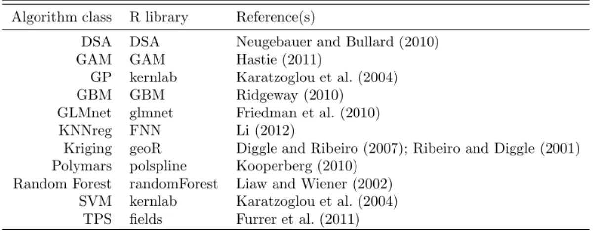
Table 1: A list of R packages used to build the Super Learner library for spatial prediction.
Algorithm class R library Reference(s)
DSA DSA Neugebauer and Bullard (2010) GAM GAM Hastie (2011)
GP kernlab Karatzoglou et al. (2004) GBM GBM Ridgeway (2010)
GLMnet glmnet Friedman et al. (2010) KNNreg FNN Li (2012)
Kriging geoR Diggle and Ribeiro (2007); Ribeiro and Diggle (2001) Polymars polspline Kooperberg (2010)
Random Forest randomForest Liaw and Wiener (2002) SVM kernlab Karatzoglou et al. (2004)
TPS fields Furrer et al. (2011)
5.1 Spatial Prediction Library
The library provided to Super Learner consisted of either 83 (number of covariates = 2) or 85 (number of covariates >2) base learners from 13 general classes of prediction algorithms. We provide a brief description of each, and list the parameter values used in the libraries. All algorithms were implemented in R (R Development Core Team, 2012). The names of the R packages used are listed in table 1.
Deletion/Substitution/Addition (DSA) performs data-adaptive polynomial regression using ν-fold cross-validation and the L2 loss (Sinisi and van der Laan, 2004). Both the
number of folds in the algorithm’s internal cross-validation and the maximum number of terms allowed in the model (excluding the intercept) were fixed to five. The maximum order of interactions was k ∈ {3,4}, and the maximum sum of powers of any single term in the model was p∈ {5,10}.
Generalized Additive Models (GAM) assume the data are generated by a model of the formE[Y|X1, . . . , Xp] =α+Pip=1fi(Xi), whereY is the outcome, (X1, . . . , Xp) are covariates
and each fi(·) is a smooth nonparametric function (Hastie, 1991). In this simulation study,
the fi(·) are cubic smoothing spline functions parametrized by desired equivalent number
of degrees of freedom, df ∈ {2,3,4,5,6}. To achieve a uniformly bounded loss function, predicted values were truncated to the range of the sampled data, plus or minus one.
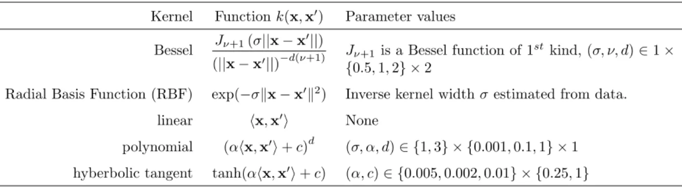
Table 2: Kernels implemented in the simulation library.hx,x0i is an inner product.
Kernel Functionk(x,x0) Parameter values Bessel Jν+1(σ||x−x
0||)
(||x−x0||)−d(ν+1) Jν+1 is a Bessel function of 1
st kind, (σ, ν, d)∈1× {0.5,1,2} ×2
Radial Basis Function (RBF) exp(−σkx−x0k2) Inverse kernel widthσestimated from data. linear hx,x0i None
polynomial (αhx,x0i+c)d (σ, α, d)∈ {1,3} × {0.001,0.1,1} ×1 hyberbolic tangent tanh(αhx,x0i+c) (α, c)∈ {0.005,0.002,0.01} × {0.25,1}
Gaussian Processes (GP) assume the observed data are normally distributed with a covariance structure that can be represented as a kernel matrix (Williams, 1999). Various implementations of the Bessel, Gaussian radial basis, linear and polynomial kernels were used. See table 2 for details about the kernel functions and parameter values. Predicted values were truncated to the range of the observed data, plus or minus one, to achieve a uniformly bounded loss function.
Generalized Boosted Modeling (GBM) combines regression trees, which model the re-lationship between an outcome and predictors by recursive binary splits, and boosting, an adaptive method for combining many weak predictors into a single prediction ensemble (Friedman, 2001). The GBM predictor can be thought of as an additive regression model fitted in a forward stage-wise fashion, where each term in the model is a simple tree. We used the following parameter values: number of trees = 10,000; shrinkage parameter λ = 0.001; bag fraction (subsampling rate) = 0.5; minimum number of observations in the terminal nodes of each tree = 10; interaction depth d∈ {1,2,3,4,5,6}, where an interaction depth of
d implies a model with up to d-way interactions.
GLMnet is a GLM fitted via penalized maximum likelihood with elastic-net mixing parameter α∈ {1/4,1/2,3/4} (Friedman et al., 2010).
K-Nearest Neighbor Regression (KNNreg) assumes the unobserved spatial process at a prediction point s0 can be well-approximated by an average of the observed spatial process values at the k nearest sampled locations to s0, k ∈ {1,5,10,20}. When k = 1 and S are
spatial locations only, this is essentially equivalent to Thiessen Polygons.
Kriging is perhaps the most commonly used spatial prediction approach. A general formulation of the spatial model assumed by Kriging can be written as Y(s) = µ(s) +
δ(s), δ(s) ∼ (0, C(θ)). The first term represents the large-scale mean trend, assumed to be deterministic and continuous. The second term is a Gaussian random function with mean zero and positive semi-definite covariance function C(θ) satisfying a stationarity as-sumption. The Kriging predictor is given as a linear combination of the observed data,
b
Ψ(s0) = Pn
i=1wi(s0)Y∗(si). The weights {wi}ni=1 are chosen so that Var
h b
Ψ(s0)−Y(s0)
i
is minimized, subject to the constraint that the predictions are unbiased. Thus, given a para-metric covariance function with known parametersθand a known mean structure, a Kriging predictor computes the best linear unbiased predictor ofY(s0). For the Kriging base learners, the parametric covariance function was assumed to be spherical,
C(h, θ) =τ2+σ2 1− 2 π sin −1 h φ +h φ s 1− h φ 2 I(h < φ).
The nugget τ2, scaleσ2, and rangeφ were estimated using Restricted Maximum Likelihood
(for details about REML, see for example Gelfand et al. (2010), chapter 4, pp 48-49). The trend was assumed to be one of the following: Constant (traditional Ordinary Kriging, OK); a first order polynomial of the locations (traditional Universal Kriging, UK); a weighted linear combination of non-location covariates only (if any); a weighted linear combination of both locations and non-location covariates (if any). All libraries contained the first and second Kriging algorithms. Libraries for simulated processes with additional covariates contained the third and fourth algorithms as well.
Multivariate adaptive polynomial spline regression (Polymars) is an adaptive regression procedure using piecewise linear splines to model the spatial process, and is parametrized by the maximum sizem = min6n1/3, n/4, 100 , where n is sample size (Stone et al., 1997).
that averages together the predictions of many regression trees constructed by drawing B
bootstrap samples and for each sample, growing an unpruned regression tree where at each node, the best split among a subset of q randomly selected covariates is chosen. In our implementation, B was set to 1000, the minimum size of the terminal nodes was 5, and the number of randomly sampled variables at each split was b√pc, where p was the number of covariates.
The library contained a number of Support Vector Machines (SVM), each implementing one of two types of regression (epsilon regression, = 0.1; or nu regression, ν = 0.2), and one of five kernels: Bessel, Gaussian radial basis, linear, polynomial, and hyperbolic tangent. The kernels are described in table 2. Predicted values were truncated to plus or minus one the range of the observed data to ensure a bounded loss, and the cost of constraints violation was fixed at 1.
Thin-plate splines (TPS) is another common approach to spatial prediction. The ob-served data are presumed to be generated by a deterministic process Y(s) = g(s), where
g(·) is an m times differentiable deterministic function with m > d/2 and dim(s) = d. The estimator of g(·) is the minimizer of a penalized sum of squares,
ˆ g = argmin g∈G n X i=1 (Yi−g(si))2+λJm(g), (2)
with d-dimensional roughness penalty
Jm(g) = Z Rd X {(v1,...,vd)} m v1, . . . , vd ∂mg(s) ∂sv1 1 . . . ∂s vd d 2 ds,
where the sum in (5.1) is taken over all nonnegative integers (v1, . . . , vd) such thatPdi=1vi =
m(Green and Silverman, 1994). The tuning parameterλ∈[0,∞) in (2) controls the permit-ted degree of roughness for bg. Asλ tends to zero, the predicted surface approaches one that exactly interpolates the observed data. Larger values ofλallow the roughness penalty term to dominate, and asλapproaches infinity,bgtends toward a multivariate least squares estimator.
In our library, the smoothing parameter was either fixed to λ ∈ {0,0.0001,0.001,0.01,0.1}
or estimated data-adaptively using Generalized Cross-validation (GCV) (see Craven and Wahba (1979) for a description of the GCV procedure). Predicted values were truncated to plus or minus one of the range of the observed data to ensure a bounded loss.
The library also contained a main terms Generalized Linear Model (GLM) and a simple empirical mean function.
5.2 Simulation Procedure
Our simulation study examined the effect of sample size (n ∈ {64,100,529}), signal-to-noise ratio (SNR), and sampling scheme. SNR was defined as the ratio of the sample variance of the spatial process and the variance of additive zero-mean normally distributed noise representing measurement error. Processes were simulated with either no added noise or with noise added to achieve a SNR of 4. We examined three sampling schemes: simple random sampling (SRS), random regular sampling (RRS), and stratified sampling (SS). Random regular samples were regularly spaced subsets of the 16,384 point grid with the initial point selected at random. Stratified random samples were taken by first dividing the domain [0,1]2 into n equal-area bins and then randomly selecting a single point from each bin.
The following procedure was repeated 100 times for each combination of spatial process, sample size, SNR level, and sampling design, giving a total of 10,800 simulations:
1. Sample n locations and any associated covariates and process values from the grid of 16,384 points in [0,1]2 ⊂
R2 according to one of the three sampling designs described
above.
2. For those simulations with SNR = 4, draw n i.i.d. samples of the random variable
ε∼N(0, σε2) and add them to thensampled process values {Y1, . . . , Yn}, whereσ2ε has
been calculated to achieve an SNR of 4.
on n: if n = 64, then ν = 64; if n = 100, then ν = 20; if n = 529, then ν = 10. Super learner uses cross-validation and theL2 loss function to estimate the risk of each
candidate predictor and returns an estimate of the optimal convex combination of the predictions made by all base learners according to their cross-validated risk.
4. For each base learner in the library and for the trained Super Learner, predict the spatial process under consideration at all unsampled points. Calculate mean squared errors (MSEs) and then divide these by the variance of the spatial process. We re-fer to this measure of performance as the Fraction of Variance Unexplained (FVU). This makes it reasonable to compare prediction performances across different spatial processes.
5.3 Simulation Results
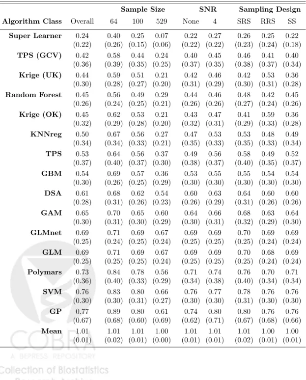
Table A.1 in Appendix A lists the average performance for each individual base learner in the library, and table 3 summarizes prediction performance for each algorithm class in the library and for Super Learner itself. Super learner was clearly the best predictor overall when comparing across broad classes, with an average FVU of 0.24 (SD = 0.22). The next best performing algorithmic class was thin-plate splines using GCV to choose the roughness penalty, with an average FVU of 0.42 (SD = 0.36). Universal Kriging (FVU = 0.44), random forest (FVU = 0.35), and Ordinary Kriging (FVU = 0.45) all performed similarly, which was slightly less well than TPS (GCV). Super Learner was also the best performer across noise conditions, sampling designs, and sample sizes, with performance improving markedly as sample size increased.
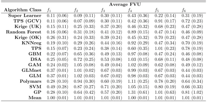
Table 4 breaks algorithmic class performance down by simulated surface. f1 was a
mean-zero GRF, something we would expect both Kriging and thin-plate splines algorithms to predict well. TPS (GCV) and Super Learner were the best performers, with nearly identical average FVUs of 0.11 (sd = 0.06). The other TPS algorithms and Universal Kriging faired slightly less well, with an average FVU of 0.15. Ordinary Kriging had an average FVU of 0.26, which was actually greater than the average FVUs for Random Forest (0.16), K-nearest
Table 3: Average FVUs (standard deviations in parentheses) from the simulation study for each algorithm class. SRS is Simple Random Sampling, RRS is Random Regular Sampling, and SS is Stratified Sampling. FVUs were calculated from predictions made on all unsampled points at each iteration. Algorithms are ordered according to overall performance.
Sample Size SNR Sampling Design Algorithm Class Overall 64 100 529 None 4 SRS RRS SS
Super Learner 0.24 0.40 0.25 0.07 0.22 0.27 0.26 0.25 0.22 (0.22) (0.26) (0.15) (0.06) (0.22) (0.22) (0.23) (0.24) (0.18) TPS (GCV) 0.42 0.58 0.44 0.24 0.40 0.45 0.46 0.41 0.40 (0.36) (0.39) (0.35) (0.25) (0.37) (0.35) (0.38) (0.37) (0.34) Krige (UK) 0.44 0.59 0.51 0.21 0.42 0.46 0.42 0.53 0.36 (0.30) (0.28) (0.27) (0.20) (0.31) (0.29) (0.30) (0.31) (0.28) Random Forest 0.45 0.56 0.49 0.29 0.44 0.46 0.48 0.42 0.45 (0.26) (0.24) (0.25) (0.21) (0.26) (0.26) (0.27) (0.24) (0.26) Krige (OK) 0.45 0.62 0.53 0.21 0.43 0.47 0.41 0.59 0.36 (0.32) (0.29) (0.28) (0.20) (0.32) (0.31) (0.29) (0.33) (0.28) KNNreg 0.50 0.67 0.56 0.27 0.47 0.53 0.53 0.48 0.49 (0.34) (0.34) (0.33) (0.21) (0.35) (0.33) (0.35) (0.33) (0.34) TPS 0.53 0.64 0.56 0.37 0.49 0.56 0.58 0.49 0.52 (0.37) (0.40) (0.37) (0.30) (0.38) (0.37) (0.40) (0.35) (0.37) GBM 0.54 0.69 0.57 0.36 0.53 0.55 0.55 0.54 0.54 (0.30) (0.26) (0.25) (0.29) (0.30) (0.30) (0.30) (0.30) (0.30) DSA 0.61 0.68 0.62 0.54 0.60 0.63 0.64 0.60 0.60 (0.28) (0.31) (0.26) (0.23) (0.26) (0.29) (0.31) (0.26) (0.26) GAM 0.65 0.70 0.65 0.60 0.64 0.66 0.68 0.63 0.64 (0.30) (0.31) (0.30) (0.29) (0.30) (0.31) (0.32) (0.29) (0.30) GLMnet 0.69 0.71 0.69 0.67 0.69 0.69 0.70 0.69 0.69 (0.25) (0.24) (0.25) (0.24) (0.25) (0.25) (0.25) (0.24) (0.24) GLM 0.69 0.71 0.69 0.67 0.69 0.69 0.70 0.68 0.69 (0.25) (0.25) (0.25) (0.24) (0.25) (0.25) (0.25) (0.24) (0.24) Polymars 0.73 0.84 0.78 0.56 0.71 0.74 0.76 0.70 0.71 (0.36) (0.40) (0.33) (0.29) (0.34) (0.38) (0.40) (0.34) (0.34) SVM 0.76 0.83 0.80 0.66 0.76 0.77 0.78 0.76 0.76 (0.30) (0.30) (0.31) (0.27) (0.30) (0.30) (0.31) (0.30) (0.30) GP 0.77 0.89 0.80 0.61 0.74 0.80 0.80 0.76 0.76 (0.67) (0.68) (0.60) (0.69) (0.62) (0.71) (0.67) (0.68) (0.66) Mean 1.01 1.01 1.01 1.00 1.01 1.01 1.01 1.00 1.00 (0.01) (0.02) (0.01) (0.00) (0.01) (0.01) (0.02) (0.01) (0.01)
Table 4: Average FVU (standard deviation in parentheses) by spatial process. Average FVU Algorithm Class f1 f2 f3 f4 f5 f6 Super Learner 0.11 (0.06) 0.09 (0.11) 0.30 (0.11) 0.43 (0.36) 0.22 (0.14) 0.31 (0.19) TPS (GCV) 0.11 (0.06) 0.07 (0.09) 0.30 (0.11) 0.42 (0.36) 0.91 (0.17) 0.72 (0.23) Krige (UK) 0.15 (0.11) 0.25 (0.33) 0.37 (0.20) 0.46 (0.32) 0.68 (0.23) 0.47 (0.28) Random Forest 0.16 (0.06) 0.31 (0.18) 0.41 (0.12) 0.89 (0.15) 0.47 (0.14) 0.46 (0.09) Krige (OK) 0.26 (0.31) 0.24 (0.33) 0.39 (0.24) 0.45 (0.32) 0.70 (0.23) 0.47 (0.28) KNNreg 0.19 (0.10) 0.29 (0.26) 0.44 (0.16) 0.92 (0.29) 0.47 (0.34) 0.70 (0.19) TPS 0.15 (0.07) 0.23 (0.24) 0.38 (0.14) 0.60 (0.35) 1.01 (0.23) 0.78 (0.19) GBM 0.22 (0.07) 0.65 (0.36) 0.49 (0.13) 0.97 (0.08) 0.47 (0.24) 0.46 (0.08) DSA 0.25 (0.05) 0.72 (0.25) 0.53 (0.08) 1.03 (0.15) 0.68 (0.11) 0.48 (0.08) GAM 0.24 (0.02) 1.05 (0.08) 0.49 (0.04) 1.02 (0.09) 0.62 (0.08) 0.49 (0.12) GLMnet 0.37 (0.01) 1.01 (0.02) 0.67 (0.03) 0.99 (0.03) 0.67 (0.03) 0.44 (0.03) GLM 0.37 (0.01) 1.02 (0.03) 0.67 (0.02) 0.98 (0.03) 0.67 (0.03) 0.44 (0.03) Polymars 0.28 (0.10) 0.94 (0.30) 0.60 (0.19) 1.11 (0.25) 0.78 (0.20) 0.64 (0.34) SVM 0.49 (0.28) 0.87 (0.27) 0.71 (0.20) 1.05 (0.15) 0.80 (0.19) 0.66 (0.33) GP 0.28 (0.10) 0.64 (0.42) 0.57 (0.20) 1.31 (0.61) 1.01 (0.63) 0.81 (1.02) Mean 1.00 (0.01) 1.01 (0.01) 1.01 (0.01) 1.00 (0.01) 1.01 (0.01) 1.01 (0.01)
neighbors regression (0.19), GBM (0.22), GAM (0.24), and DSA (0.25).
f2 was a simple sinusoidal surface, another functional form where we would expect
thin-plate splines to excel, provided the samples properly captured the periodicity of the process. TPS (GCV) had the best overall performance, with an average FVU of 0.07 (sd = 0.09). Super Learner performed only slightly less well, with an average FVU of 0.09 (sd = 0.11). The other TPS algorithms (0.23), Ordinary Kriging (0.24) and Universal Kriging (0.25) performed substantially less well on average.
f3 was a relatively complex function involving a ”cyclone” Gaussian random field and a
distance decay function of randomly selected points. Once again, the average performances of TPS (GCV) and Super Learner were nearly identical (FVU = 0.30, sd- 0.11).
f4 was a smooth, heterogeneous process. TPS (GCV) (average FVU = 0.42), Super
Learner (0.43), Ordinary Kriging (0.45), and Universal Kriging (0.46) all performed similarly.
f5was a clustered, rough surface we would expect to be well-suited to K nearest neighbors,
GBM, and Random Forest. In fact, all three of these algorithmic classes had nearly identical performances, with an average FVU of 0.47. Super Learner, however, had an average FVU of 0.22 (sd = 0.14), which was dramatically better than any of the other algorithmic classes.
The Ordinary (average FVU = 0.70) and Universal (0.68) Kriging algorithms had similar average performances to GAM (0.62), GLM (0.67), GLMnet (0.67), and DSA (0.68). Not surprisingly, TPS (GCV) and TPS with fixed λ did poorly, with average FVUs of 0.91 and 1.01, respectively.
f6 was a somewhat rough surface constructed from a Gaussian random field and
point-source distance decay functions. As expected, Kriging with trend w1, . . . , w6 had the best
performance on average, with an FVU of 0.25 (sd = 0.14), closely followed by Kriging with trends, w1, . . . , w6 (average FVU = 0.26, sd=0.15). Super Learner had the next best average
performance, with an average FVU of 0.31 (sd = 0.19). GLM, GLMnet, GBM, Random Forest, the Ordinary and Universal Kriging algorithms, and DSA all performed similarly slightly less well, with average FVUs from 0.44 to 0.48. The TPS (GCV) and TPS with fixed
λ were at a disadvantage given the roughness of the surface, with average FVUs of 0.72 and 0.78, respectively.
These simulation results clearly illustrate some of the chief advantages of Super Learner as a spatial predictor. For surfaces that were perfectly suited for one or more base learners in the library, Super Learner either performed almost as well as the best base learner, or it outperformed its library. For more complex, rougher surfaces, Super Learner performed significantly better than any single base learner in the library. It had the best overall perfor-mance even at the smallest sample size, and appeared to be relatively insensitive to sampling strategy.
6. PRACTICAL DATA EXAMPLE: PREDICTING LAKE ACIDITY
We applied Super Learner to a lake acidity data set previously analyzed by Gu (2002) and Huang and Chen (2007). Increases in water acidity are known to have a deleterious effect on lake ecology. Having an accurate estimate of the spatial distribution of lake acidity is an essential first step toward crafting effective regulatory interventions to control it. The data were sampled by the U.S. Environmental Protection Agency during the Fall of 1984 in the
longitudes and latitudes (in degrees), calcium ion concentrations (in milligrams per liter), and pH values. The EPA used a systematic stratified sampling design which we treated as fixed here. Because only one sample per lake was collected, we assume some measurement error that is independent of lake pH, calcium ion concentration, and spatial location. The data are freely available in the R package gss (Gu, 2012). We used the same nearly equal area projection as Gu (2002) and Huang and Chen (2007),
x1 = cos((πxlat)/180) sin(π(xlon−xlon)/180)
x2 = sin(π(xlat−xlat)/180),
where xlat and xlon are the midpoints of the latitude and longitude ranges, respectively.
Let xi = (xi,1, xi,2) denote the ith sampling location; wi denote the calcium ion
concen-tration observed at the ith sampling location; and Yi∗ be the pH value observed at the ith
sampling location. We assume thatE[Yi∗|Si =s] =Y(s), where Si = (xi, wi). Our objective
is to learn the lake pH spatial process from the data.
The library used to predict lake acidity was similar in composition to the simulation library described in subsection 5.1, with some important differences. We reduced the number of parameterizations for some of the algorithm classes in the library. We used one DSA learner, which used 10-fold cross-validation and considered polynomials of up to five terms (m = 5), each term being at most a two-way interaction (k = 2) with a maximum sum of powersp= 3. We used a reduced the number of parameterizations of GAM, GBM, TPS, GP, and SVM learners, as well. We also included screening algorithms that allowed us to train learners on specific subsets of covariates: x, w, logw, (x, w), and (x,logw). We considered theL2loss function, and the predictions from all base learners were truncated to the observed
pH range in order to ensure a uniformly bounded loss.
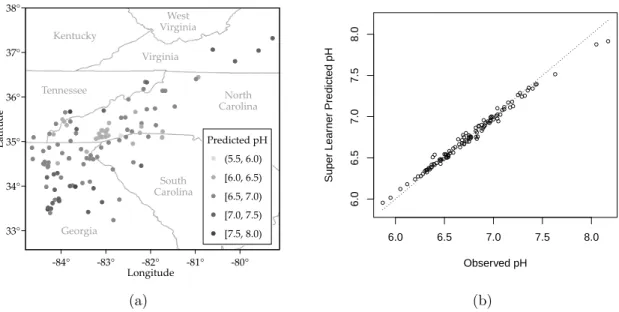
Table A.2 in Appendix A provides a detailed list of the library and shows performance results for each base learner as well as Super Learner. Figure 2 provides graphical represen-tations of Super Learner’s pH predictions. Many of the algorithms in the library performed
slightly better when given logw as opposed to w, but for those algorithms like GBM and Random Forest that were not attempting to fit some kind of polynomial trend, logging the calcium ion concentration made little difference in performance. As expected, most algo-rithms had cross-validated risk estimates that were worse than their empirical risk estimates calculated from predictions made after training on the full data set. The Kriging algorithms, for instance, were all exact interpolators when trained on the full data, and thus had esti-mated empirical MSEs of 0, whereas their MSEs estiesti-mated via cross-validation ranged from 0.07 (FVU = 0.46) to 0.11 (FVU = 0.72). The Gaussian processes with RBF kernel had the most pronounced differences between the two risk estimates. For example, GP (RBF) trained on the covariates (x, w) had an empirical MSE of 0.01 (FVU = 0.08) and a cross-validated MSE of 0.22 (FVU = 1.46).
The Super Learner algorithm gave non-zero weights to the predictions of eight base learn-ers from five different algorithm classes: GBM, KNNreg, Kriging, Random Forest, and SVM (polynomial kernel). While the largest weight went to an exactly interpolating algorithm (Kriging with trend term logw, β = 0.58), Super Learner pH predictions are a slightly smoothed version of the observed data, with attenuated predictions for the highest and lowest observations.
7. CONCLUSION/DISCUSSION
In this article, we have demonstrated the use of an ensemble learner for spatial prediction that uses cross-validation to optimally combine the predictions from multiple, heterogeneous base learners. We have reviewed important theoretical results giving performance bounds that imply Super Learner will perform asymptotically at least as well as the best candidate in the library. We discussed the assumptions required for these optimality properties hold. These assumptions are reasonable for many measurement error scenarios and commonly im-plemented spatial sampling designs, including various forms of stratified and random regular sampling. In this paper, we have not addressed dependent sampling designs, where sampling
‐80° ‐81° ‐82° ‐83° ‐84° 38° 37° 36° 35° 34° 33° Predicted pH (5.5, 6.0) [6.0, 6.5) [6.5, 7.0) [7.0, 7.5) [7.5, 8.0) North Carolina South Carolina Georgia Tennessee Virginia Kentucky West Virginia Longitude La titu de (a) ● ● ● ● ● ● ● ● ● ● ● ● ● ● ● ● ● ● ● ● ● ● ●● ● ● ● ●●● ●● ● ● ● ● ● ●● ● ● ● ● ●● ●● ● ● ● ● ● ●● ● ● ● ● ●● ● ●● ● ● ● ● ●● ● ● ● ●● ● ● ● ● ● ● ● ● ● ● ● ● ● ● ● ● ● ● ●● ● ● ● ● ● ● ● ● ● ● ● ● ● ● ● ● ● ● 6.0 6.5 7.0 7.5 8.0 6.0 6.5 7.0 7.5 8.0 Observed pH Super Lear ner Predicted pH (b)
Figure 2: (a) A map of Super Learner’s pH predictions, and (b) a plot of Super Learner’s predic-tions as a function of the observed data. Super Learner mildly attenuated the pH values at either end of the range, but otherwise provided a fairly close fit to the data.
area for future research. We also limited our scope to the case where measurement error is at least conditionally mean-zero. Spatially structured measurement error that is not condi-tionally mean zero is a common problem in many spatial prediction applications, and there have been a number of attempts to alter the cross-validation procedure to accommodate it (Francisco-Fernandez and Opsomer, 2005; Carmack et al., 2009). These proposed techniques generally require one to estimate the error correlation structure from the data or to know it a priori. How well these algorithms perform if the correlation extent is substantially under-estimated is unknown. Ideally, it would be best to have a stronger theoretical understanding of how the degree of dependence between training and validation sets affects cross-validated risk estimates both asymptotically and in finite samples. This is an important future area for research.
APPENDIX A. TABLES
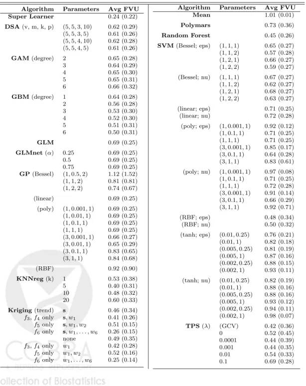
Table A.1: Simulation results for full library. For each algorithm, average Fraction of Variance Unexplained, (Avg FVU, standard deviation in parentheses) is the FVU averaged over all spatial processes, sample sizes, sampling designs, and noise condidtions. At each iteration, MSEs were calculated using all unsamped locations. Note that of the eight Kriging algorithms, only two were used to predict all spatial processes.
Algorithm Parameters Avg FVU
Super Learner 0.24 (0.22) DSA(v, m, k, p) (5,5,3,10) 0.62 (0.29) (5,5,3,5) 0.61 (0.26) (5,5,4,10) 0.62 (0.28) (5,5,4,5) 0.61 (0.26) GAM(degree) 2 0.65 (0.28) 3 0.64 (0.29) 4 0.65 (0.30) 5 0.65 (0.31) 6 0.66 (0.32) GBM(degree) 1 0.64 (0.28) 2 0.56 (0.28) 3 0.53 (0.30) 4 0.52 (0.30) 5 0.51 (0.31) 6 0.50 (0.31) GLM 0.69 (0.25) GLMnet(α) 0.25 0.69 (0.25) 0.5 0.69 (0.25) 0.75 0.69 (0.25) GP(Bessel) (1,0.5,2) 1.12 (1.52) (1,1,2) 0.81 (0.81) (1,2,2) 0.74 (0.67) (linear) 0.69 (0.25) (poly) (1,0.001,1) 0.69 (0.25) (1,0.01,1) 0.69 (0.25) (1,0.1,1) 0.69 (0.25) (1,1,1) 0.69 (0.25) (3,0.001,1) 0.66 (0.27) (3,0.01,1) 0.65 (0.29) (3,0.1,1) 0.83 (0.65) (3,1,1) 0.84 (0.68) (RBF) 0.92 (0.90) KNNreg(k) 1 0.53 (0.38) 5 0.40 (0.31) 10 0.48 (0.32) 20 0.60 (0.33) Kriging(trend) s 0.46 (0.34) f3,f4only s, w1 0.41 (0.26) f5only s, w1, w2 0.51 (0.15) f6only s, w1, . . . , w6 0.26 (0.15) none 0.49 (0.35) f3,f4only w1 0.42 (0.28) f5only w1, w2 0.52 (0.16) f6only w1, . . . , w6 0.25 (0.14)
Algorithm Parameters Avg FVU
Mean 1.01 (0.01) Polymars 0.73 (0.36) Random Forest 0.45 (0.26) SVM(Bessel; eps) (1,1,1) 0.65 (0.27) (1,1,2) 0.57 (0.28) (1,2,1) 0.66 (0.27) (1,2,2) 0.59 (0.27) (Bessel; nu) (1,1,1) 0.67 (0.27) (1,1,2) 0.62 (0.27) (1,2,1) 0.68 (0.27) (1,2,2) 0.63 (0.27) (linear; eps) 0.71 (0.25) (linear; nu) 0.72 (0.28) (poly; eps) (1,0.001,1) 0.92 (0.12) (1,0.1,1) 0.71 (0.25) (1,1,1) 0.71 (0.25) (3,0.001,1) 0.85 (0.17) (3,0.1,1) 0.64 (0.28) (3,1,1) 0.83 (0.61) (poly; nu) (1,0.001,1) 0.97 (0.08) (1,0.1,1) 0.71 (0.25) (1,1,1) 0.72 (0.28) (3,0.001,1) 0.91 (0.14) (3,0.1,1) 0.66 (0.29) (3,1,1) 0.92 (0.71) (RBF; eps) 0.48 (0.34) (RBF; nu) 0.50 (0.32) (tanh; eps) (0.01,0.25) 0.76 (0.21) (0.01,1) 0.82 (0.18) (0.005,0.25) 0.81 (0.19) (0.005,1) 0.87 (0.16) (0.002,0.25) 0.88 (0.15) (0.002,1) 0.93 (0.11) (tanh; nu) (0.01,0.25) 0.82 (0.19) (0.01,1) 0.88 (0.16) (0.005,0.25) 0.88 (0.16) (0.005,1) 0.93 (0.12) (0.002,0.25) 0.94 (0.11) (0.002,1) 0.98 (0.07) TPS(λ) (GCV) 0.42 (0.36) 0 0.52 (0.45) 0.0001 0.44 (0.39) 0.001 0.44 (0.35) 0.01 0.54 (0.33) 0.1 0.69 (0.28)
Table A.2: Lake acidity results for full library.S denotes the variable subset each algorithm was given. Risks were estimated via cross-validation (CV) or on the full dataset (Full). β are the convex weights assigned to each algorithm in the Super Learner predictor.
\ MSE FVU\ Algorithm S CV Full β Super Learner 0.00 (0.03) DSA x, w 0.13 (0.85) 0.12 (0.80) 0 x, w` 0.09 (0.57) 0.07 (0.46) 0 GAM(degree) 2 x, w 0.09 (0.58) 0.07 (0.49) 0 x, w` 0.08 (0.51) 0.07 (0.45) 0 3 x, w 0.08 (0.54) 0.07 (0.43) 0 x, w` 0.08 (0.51) 0.06 (0.41) 0 4 x, w 0.08 (0.53) 0.06 (0.40) 0 x, w` 0.08 (0.50) 0.06 (0.39) 0 GBM(degree) 2 x, w 0.07 (0.49) 0.05 (0.32) 0 x, w` 0.07 (0.49) 0.05 (0.32) 0 4 x, w 0.08 (0.50) 0.04 (0.29) 0 x, w` 0.07 (0.49) 0.05 (0.32) 0 6 x, w 0.07 (0.49) 0.04 (0.28) 0.12 x, w` 0.07 (0.49) 0.04 (0.29) 0 GLM x, w 0.11 (0.74) 0.10 (0.67) 0 x, w` 0.08 (0.54) 0.08 (0.50) 0 GLMnet(α) 0.25 x, w 0.12 (0.79) 0.10 (0.67) 0 x, w` 0.08 (0.55) 0.08 (0.50) 0 0.5 x, w 0.11 (0.73) 0.10 (0.67) 0 x, w` 0.08 (0.54) 0.08 (0.50) 0 0.75 x, w 0.11 (0.75) 0.10 (0.67) 0 x, w` 0.08 (0.54) 0.08 (0.50) 0 GP(Bessel) (1, 0.5, 2) x, w 0.13 (0.83) 0.04 (0.25) 0 x, w` 0.16 (1.03) 0.03 (0.21) 0 (1, 1, 2) x, w 0.14 (0.90) 0.04 (0.27) 0 x, w` 0.15 (0.97) 0.03 (0.22) 0 (1, 2, 2) x, w 0.16 (1.08) 0.04 (0.29) 0 x, w` 0.17 (1.10) 0.04 (0.25) 0 GP(linear) x, w 0.11 (0.74) 0.10 (0.67) 0 x, w` 0.08 (0.54) 0.08 (0.50) 0 GP(RBF) x, w 0.22 (1.45) 0.02 (0.16) 0 x, w` 0.22 (1.46) 0.01 (0.08) 0 GP(poly.) (1, 0.001, 1) x, w 0.11 (0.74) 0.10 (0.67) 0 x, w` 0.08 (0.54) 0.08 (0.50) 0 (1, 0.01, 1) x, w 0.11 (0.74) 0.10 (0.67) 0 x, w` 0.08 (0.54) 0.08 (0.50) 0 (1, 0.1, 1) x, w 0.11 (0.74) 0.10 (0.67) 0 x, w` 0.08 (0.54) 0.08 (0.50) 0 (1, 1, 1) x, w 0.11 (0.74) 0.10 (0.67) 0 x, w` 0.08 (0.54) 0.08 (0.50) 0 \ MSEFVU\ Algorithm S CV Full β KNNreg(k) 1 x 0.17 (1.12) 0.00 (0.00) 0.02 x, w 0.11 (0.73) 0.00 (0.00) 0.08 5 x 0.12 (0.76) 0.08 (0.52) 0 x, w 0.08 (0.55) 0.06 (0.38) 0.04 10 x 0.11 (0.73) 0.09 (0.61) 0 x, w 0.08 (0.53) 0.07 (0.43) 0 20 x 0.11 (0.72) 0.10 (0.66) 0.03 x, w 0.09 (0.56) 0.08 (0.50) 0 Kriging (OK) 0.11 (0.71) 0.00 (0.00) 0 w 0.09 (0.56) 0.00 (0.00) 0 w` 0.07 (0.46) 0.00 (0.00) 0.58 (UK) x 0.11 (0.72) 0.00 (0.00) 0 x, w 0.09 (0.60) 0.00 (0.00) 0 x, w` 0.08 (0.51) 0.00 (0.00) 0 Mean 0.15 (1.00) 0.15 (1.00) 0 Polymars x, w 0.10 (0.63) 0.04 (0.27) 0 x, w` 0.08 (0.56) 0.05 (0.36) 0 RF x, w 0.08 (0.50) 0.02 (0.11) 0.06 x, w` 0.08 (0.50) 0.02 (0.12) 0 SVM(Bessel; eps) (1, 1, 2) x, w 0.09 (0.57) 0.06 (0.43) 0 x, w` 0.08 (0.55) 0.06 (0.42) 0 (1, 2, 1) x, w 0.09 (0.56) 0.08 (0.51) 0 x, w` 0.08 (0.52) 0.07 (0.46) 0 (1, 2, 2) x, w 0.09 (0.56) 0.07 (0.45) 0 x, w` 0.08 (0.55) 0.07 (0.44) 0 SVM(Bessel; nu) (1, 1, 2) x, w 0.09 (0.57) 0.07 (0.48) 0 x, w` 0.09 (0.61) 0.07 (0.46) 0 (1, 2, 1) x, w 0.1 (0.64) 0.08 (0.56) 0 x, w` 0.08 (0.56) 0.07 (0.48) 0 (1, 2, 2) x, w 0.09 (0.59) 0.07 (0.49) 0 x, w` 0.09 (0.58) 0.07 (0.47) 0 SVM(poly, eps) (1, 0.001, 1) x, w 0.15 (0.97) 0.14 (0.96) 0 x, w` 0.14 (0.94) 0.14 (0.92) 0 (1, 0.1, 1) x, w 0.12 (0.78) 0.10 (0.69) 0 x, w` 0.08 (0.52) 0.08 (0.50) 0 (1, 1, 1) x, w 0.12 (0.78) 0.11 (0.69) 0 x, w` 0.08 (0.53) 0.08 (0.50) 0.08 (3, 0.001, 1) x, w 0.14 (0.92) 0.13 (0.89) 0 x, w` 0.12 (0.81) 0.12 (0.78) 0 SVM(poly, nu) (1, 0.001, 1) x, w 0.15 (0.98) 0.15 (0.97) 0 x, w` 0.15 (0.97) 0.14 (0.95) 0 (1, 0.1, 1) x, w 0.11 (0.73) 0.11 (0.70) 0 x, w` 0.08 (0.55) 0.08 (0.53) 0 (1, 1, 1) x, w 0.11 (0.74) 0.11 (0.70) 0 x, w` 0.08 (0.54) 0.08 (0.52) 0 (3, 0.001, 1) x, w 0.14 (0.94) 0.14 (0.92) 0 x, w` 0.13 (0.89) 0.13 (0.87) 0 TPS(GCV) x 0.11 (0.71) 0.08 (0.53) 0
APPENDIX B. ORACLE INEQUALITY FOR INDEPENDENT, NONIDENTICAL EXPERIMENTS AND QUADRATIC LOSS
Let On = (O1, . . . , On) ∼ P0n be a vector of independent, nonidentical observations, where
eachOi = (Xi, Yi) consists of two components: ad-dimensional covariate vectorXi ∈Rd, and
a univariate outcomeYi ∈R. We associate with eachOi an index si ∈S. The true unknown
data generating distribution for eachOiis denotedP0,Oi(O) =P0,O|S(O|si)∈ {P0,O|s:s∈S}.
LetPs,O be the joint distribution of (S, O), defined by a degenerate marginal distribution of
S,I(S =s), and the conditional distribution ofO givenS =s,PO|s. We can formulateOnas
nindependent draws (Si, Oi)∼P0,(si,Oi),i= 1, . . . , n, with empirical probability distribution
Pn. LetMbe a set of possible probability distributions ofPO|S. Define a parameter Ψ : M →
Ψ, and letψ0 = Ψ(P0,O|S) be the true value of that parameter. LetBn ∈ {0,1}nbe a random
vector indicating splits into a training sample, {i : Bn(i) = 0}, and validation sample, {i :
Bn(i) = 1}. Let p=Pni=1Bn(i) be the proportion of observations in the validation sample,
and letP0
n,Bn andP 1
n,Bn be the empirical distributions of the training and validation samples,
respectively. Define an average joint distribution: P10,Bn = (np)−1P
i:Bn(i)=1P0,(si,Oi). Let
L(ψ)(S, O) be a loss function such that for all i, P0,(si,O)L(ψ0) = minψ∈ΨP0,(si,Oi)L(ψ). Let
{Ψbk(Pn) : k = 1, . . . , Kn} be a set of Kn estimators of ψ0. Assume P(Ψbk(Pn) ∈ Ψ) = 1 for
all k = 1, . . . , Kn. We write the true cross-validated risk of ψ0 as Θeopt =EBn
P10,BnL(ψ0)
. We denote the true conditional cross-validated risk of any estimator Ψbk as
e Θn(1−p)(k)≡EBn h P10,BnLΨbk Pn,0Bni =EBn 1 np X i:Bn(i)=1 P0,(Oi|si)L b Ψk Pn,0Bn (si, Oi) ,
and a benchmark (oracle) selector as ˜kn(1−p) = argminkΘen(1−p)(k).
We denote the cross-validated risk of any estimator Ψbk as
b Θn(1−p)(k)≡EBn h Pn,1BnL b ΨPn,0Bn i =EBn 1 np X L b ΨPn,0Bn (si, Oi) ,
and the cross-validation selector as kn = argmink Θbn(1−p)(k). Finally, we define a loss-based dissimilarity dn(ψ, ψ0)≡EBn h P10,B n L[ψ]−L[ψ0] i . Assumptions.
A1. There exists a real-valued M1∗ <∞such that supψ∈Ψ
supi,si,OiL(ψ)(si, Oi)−L(ψ0)(si, Oi)
≤ M1∗, where the supremum over Oi
is taken over the support of the distribution P0,Oi|si of Oi.
A2. There exists a real-valued M2 <∞such that
sup i,ψ∈Ψ ( VarP0,(si,Oi) L(ψ)−L(ψ0) (S, O) EP0,(si,Oi) L(ψ)−L(ψ0) (S, O) ) ≤M2.
Definitions.We define the following constants:M1 = 2M1∗;C(M1, M2, δ)≡2(1+δ)2 M31 +Mδ2
. Finite sample result. For anyδ >0, we have
E h dn b Ψkn Pn,0Bn, ψ0 i ≤ (1 + 2δ)Ehdn b Ψ˜k n(1−p) Pn,0Bn, ψ0 i + 2C(M1, M2, δ) 1 + logKn np . (B.1)
Asymptotitic implications. (B.1) has the following asymptotic implications:
logKn npEhΘen(1−p) ˜ kn(1−p) −Θeopt i n→∞ −−−→0 =⇒ E h e Θn(1−p)(kn)−Θeopt i E h e Θn(1−p) ˜ kn(1−p) −Θeopt i n→∞ −−−→1. logKn np e Θn(1−p) ˜ kn(1−p) −Θeopt p − →0 =⇒ Θen(1−p)(kn)−Θeopt e Θn(1−p) ˜ kn(1−p) −Θeopt p − →1. (B.2)
(B.2) follows from the fact that, given a sequence of random variables X1, X2, . . ., and a
positive functiong[n],E|Xn|=O(g[n]) impliesXn=OP(g[n]). This is a direct consequence
Proof of theorem. We have 0≤Θen(1−p)(kn)−Θeopt (B.3a) =EBn h P10,Bn n L b Ψkn Pn,0Bn −L(ψ0) oi −(1 +δ)EBn h Pn,1Bn n L b Ψkn Pn,0Bn −L(ψ0) oi + (1 +δ)EBn h Pn,1BnnLΨbkn Pn,0Bn−L(ψ0) oi ≤EBn h P10,BnnLΨbkn Pn,0Bn−L(ψ0) oi (B.3b) −(1 +δ)EBn h Pn,1BnnLΨbkn Pn,0Bn−L(ψ0) oi + (1 +δ)EBn h Pn,1BnnLΨbk˜ n(1−p) Pn,0Bn−L(ψ0) oi =EBn h P10,BnnLΨbkn Pn,0Bn−L(ψ0) oi (B.3c) −(1 +δ)EBn h Pn,1BnnLΨbkn Pn,0Bn−L(ψ0) oi (B.3d) + (1 +δ)EBn h Pn,1BnnLΨbk˜ n(1−p) Pn,0Bn−L(ψ0) oi (B.3e) −(1 + 2δ)EBn h Pn,1BnnLΨbk˜ n(1−p) Pn,0Bn−L(ψ0) oi (B.3f) + (1 + 2δ)EBn h Pn,1BnnLΨb˜k n(1−p) Pn,0Bn−L(ψ0) oi (B.3g)
(B.3a) follows from the definition of Θeopt. (B.3b) follows from the definition of the
cross-validation selector kn, such that for all k, Θbn(1−p)(kn)≤Θbn(1−p)(k). Let Rn,kn represent the
first two terms in the last expression, (B.3c) and (B.3d). Let Tn,˜kn(1−p) represent the second
two terms of the last expression, (B.3e) and (B.3f). The last term, (B.3g), is the benchmark and can be written as (1 + 2δ)hΘen(1−p)
˜ kn(1−p)−Θeopt i . Hence, 0≤Θen(1−p)(kn)−Θeopt≤(1 + 2δ) h e Θn(1−p) ˜ kn(1−p)−Θeopt i +Rn,kn+Tn,k˜n(1−p). (B.4)
the following notation: b Hk ≡Pn,1Bn n LΨbk Pn,0Bn−L(ψ0) o e Hk ≡P 1 0,Bn n LΨbk Pn,0Bn−L(ψ0) o Rn,k(Bn)≡(1 +δ) h e Hk−Hbk i −δHek Tn,k(Bn)≡(1 +δ) h b Hk−Hek i −δHek
Note that Rn,k =EBn[Rn,k(Bn)];Tn,k =EBn[Tn,k(Bn)]; and that by definition ofψ0,Hek≥0
for all k. Note also that given an arbitrary k ∈ {1, . . . Kn},
PRn,kn(Bn)> s|Pn,0Bn,Bn =P " e Hkn −Hkn > s+δHekn 1 +δ Pn,0Bn,Bn # ≤Knmax k P " e Hk−Hbk> s+δHek 1 +δ Pn,0Bn,Bn # . Similarly forTn,˜kn(1−p)(Bn), P h Tn,˜k n(1−p)(Bn)> s|P 0 n,Bn,Bn i =Knmax k P " b Hk−Hek > s+δHek 1 +δ Pn,0Bn,Bn # . Conditional on P0
n,Bn andBn, consider the np random variables for whichBn(i) = 1, Zk,i≡ n LΨbk P0 n,Bn −L(ψ0) o
(si, Oi). We can rewrite Hbk and Hek in terms of Zk,i,
b Hk= 1 np np X i=1 Zk,i, e Hk= 1 np np X i=1 EZk,i|Pn,0Bn,Bn .
Then Hek−Hbk is the sum of np mean zero centered random variables. By assumption A1
also have σ2 k,i≡Var Zk,i|Pn,0Bn,Bn ≤M2EZk,i|Pn,0Bn,Bn , which implies σk2 ≡ 1 np np X i=1 σk,i2 ≤M2 1 np np X i=1 EZk,i|Pn,0Bn,Bn =M2Hek.
We will apply Bernstein’s inequality to the centered empirical mean Hek−Hbk and obtain
a tail probability bounded by exp{−npq/c}, where c is a finite, real-valued constant. This will show that the risk dissimilarities converge at a rate of (logKn)/np. We state Bernstein’s
inequality for ease of reference. A proof is given in Lemma A.2 on page 594 in Gy¨orfi et al. (2002).
Lemma 1 Bernstein’s inequality.
Let Zi, i = 1, . . . , n be independent, real valued random variables such that Zi ∈ [a, b] with
probability one. Let 0<Pn
i=1Var(Zi)/n≤σ
2. Then, for all >0,
P 1 n n X i=1 (Zi−EZi)> ! ≤exp − n2 2(σ2+(b−a)/3) . This implies P 1 n n X i=1 (Zi−EZi)> ! ≤2 exp − n2 2(σ2+(b−a)/3) .
By Bernstein’s lemma, for q >0,
PRn,k(Bn)> q|Pn,0Bn,Bn =P e Hk−Hbk > 1 1 +δ q+δHek P 0 n,Bn,Bn ≤P e Hk−Hbk > 1 1 +δ q+δσ 2 k M2 P 0 n,Bn,Bn ≤exp ( − np 2[1 +δ]2 [q+δσ2 k/M2] 2 σ2 k+ M1 3(1+δ)[q+δσ 2 k/M2] !) .
Note that [q+δσ2 k/M2] 2 σ2 k+ M1 3(1+δ)[q+δσ 2 k/M2] = [s+δσ 2 k/M2] 2 σ2 k q+σk2/M2 + M1 3(1+δ) ≥ [s+δσ 2 k/M2] 2 M2 δ + M1 3 ≥ M s 2 δ + M1 3 .
This shows that for q >0,
PRn,kn(Bn)> q Pn,0B n,Bn ≤Knexp{(−npq)/C(M1, M2, δ)}.
In particular, this provides us with a bound for the marginal probability of Rn,kn(Bn),
P[Rn,kn(Bn)> q]≤Knexp{(−npq)/C(M1, M2, δ)}.
As in the proof of theorem 1 in van der Laan et al. (2004) and Dudoit and van der Laan (2005), for each u >0, we have
E[Rn,kn]≤u+
Z ∞
u
Knexp{(−npq)/C(M1, M2, δ)}dq.
The minimum is attained atun =C(M1, M2, δ) logKn/npand is given byC(M1, M2, δ)(logKn+
1)/np. Thus ERn,kn ≤C(M1, M2, δ)(1 + logKn)(np). The same applies for ETn,˜kn(1−p).
Taking the expected values of the quantities in (B.4) yields the following finite sample result: 0≤EhΘen(1−p)(kn) i −Θeopt ≤(1 + 2δ)EhΘen(1−p) i −Θeopt + 2C(M1, M2, δ) 1 + logKn np .
This completes the proof.
REFERENCES
Arlot, S. and Celisse, A. (2010). A Survey of Cross-validation Procedures for Model Selection.
Breiman, L. (1996). Stacked Regressions. Machine Learning, 24(1):49–64.
Breiman, L. (2001). Random Forests. Machine Learning, 45(1):5–32.
Carmack, P. S., Schucany, W. R., Spence, J. S., Gunst, R. F., Lin, Q., and Haley, R. W. (2009). Far Casting Cross-validation. Journal of Computational and Graphical Statistics, 18(4):879–893.
Chen, J. and Wang, C. (2009). Using Stacked Generalization to Combine SVMs in Magnitude and Shape Feature Spaces for Classification of Hyperspectral Data. IEEE Transactions on Geoscience and Remote Sensing, 47(7):2193–2205.
Craven, P. and Wahba, G. (1979). Smoothing Noisy Data with Spline Functions: Estimating the Correct Degree of Smoothing by the Method of Generalized Cross-validation. Nu-merische Mathematik, 31:377–403.
Cressie, N. A. C. (1993). Statistics for Spatial Data. Wiley Series in probability and math-ematical statistics. John Wiley and Sons, Inc., revised edition.
Davis, B. M. (1987). Uses and Abuses of Cross-Validation in Geostatistics. Mathematical Geology, 19(3):241–248.
Diggle, P. J. and Ribeiro, Jr., P. (2007). Model Based Geostatistics. Springer, New York.
Dudoit, S. and van der Laan, M. J. (2005). Asymptotics of Cross-validated Risk Estimation in Estimator Selection and Performance Assessment. Statistical Methodology, 2(2):131–154.
Ellers, J. M., Landers, D. H., and Brakke, D. F. (1988). Chemical and Physical Character-istics of Lakes in the Southeastern United States. Environmental Science and Technology, 22(2):172–177.
Francisco-Fernandez, M. and Opsomer, J. D. (2005). Smoothing Parameter Selection Meth-ods for Nonparametric Regression with Spatially Correlated Errors.The Canadian Journal
Friedman, J., Hastie, T., and Tibshirani, R. (2010). Regularization Paths for Generalized Linear Models via Coordinate Descent. Journal of Statistical Software, 33(1).
Friedman, J. H. (2001). Greedy Function Approximation: a gradient boosting machine.
Annals of Statistics, 29(5):367–378.
Furrer, R., Nychka, D., and Sain, S. (2011). fields: Tools for spatial data. R package version 6.6.1.
Geisser, S. (1975). The predictive sample reuse method with applications. Journal of the American Statistical Association, 70(350):320–328.
Gelfand, A. E., Diggle, P. J., Fuentes, M., and Guttorp, P., editors (2010). Handbook of Spatial Statistics. CRC Press.
Green, P. and Silverman, B. (1994). Nonparametric Regression and Generalized Linear Models. Number 58 in Monographs on Statistics and Applied Probability. Chapman & Hall/CRC.
Gu, C. (2002). Smoothing spline ANOVA models. Springer - New York.
Gu, C. (2012). gss: General Smoothing Splines. R package version 2.0-11.
Gy¨orfi, L., Kohler, M. A. K., and Walk, H. (2002). A Distribution-free Theory of Nonpara-metric Regression. Springer Series in Statistics. Springer.
Hastie, T. (2011). gam: Generalized Additive Models. R package version 1.04.1.
Hastie, T. J. (1991). Statistical models in S, chapter 7: Generalized Additive Models. Wadsworth and Brooks/Cole.
Huang, H.-C. and Chen, C.-S. (2007). Optimal Geostatistical Model Selection. Journal of the American Statistical Association, 102(479):1009–1024.
Jiang, W. (2009). On Uniform Deviations of General Empirical Risks with Unboundedness, Dependence, and High Dimensionality. Journal of Machine Learning Research, 10:977– 996.
Karatzoglou, A., Smola, A., Hornik, K., and Zeileis, A. (2004). kernlab – an S4 package for kernel methods in R. Journal of Statistical Software, 11(9):1–20.
Kleiber, W., Raftery, A. E., and Gneiting, T. (2011). Geostatistical model averaging for lo-cally calibrated probabilistic quantitative precipitation forecasting. Journal of the Amer-ican Statistical Association, 106(496):1291–1303.
Kooperberg, C. (2010). polspline: Polynomial spline routines. R package version 1.1.5.
LeBlanc, M. and Tibshirani, R. (1996). Combining estimates in regression and classification.
Journal of the American Statistical Association, 91:1641–1650.
Li, S. (2012). FNN: Fast Nearest Neighbor Search Algorithms and Applications. R package version 0.6-3.
Liaw, A. and Wiener, M. (2002). Classification and regression by randomforest. R News, 2(3):18–22.
Lumley, T. (2005). An empirical process limit theorem for sparsely correlated data. UW Biostatistics Working Paper Series, (255).
Mat´ern, B. (1986). Spatial Variation. Springer - New York, 2nd edition.
Neugebauer, R. and Bullard, J. (2010). DSA: Deletion/Substitution/Addition algorithm. R package version 3.1.4.
Opsomer, J., Wang, Y., and Yang, Y. (2001). Nonparametric regression with correlated errors. Statistical Science, 16(2):134–153.
Polley, E. C., Rose, S., and van der Laan, M. J. (2011). Targeted Learning: Casual Infer-ence for Observational and Experimental Data, chapter 3: Super Learning, pages 43–65. Springer, New York.
Polley, E. C. and van der Laan, M. J. (2010). Super learner in prediction. U.C. Berkeley Division of Biostatistics Working Paper Series.
R Development Core Team (2012). R: A Language and Environment for Statistical Com-puting. R Foundation for Statistical Computing, Vienna, Austria.
Ribeiro, Jr., P. J. and Diggle, P. J. (2001). geoR: a package for geostatistical analysis.
R-NEWS, 1(2):14–18.
Ridgeway, G. (2010).gbm: Generalized Boosted Regression Models. R package version 1.6-3.1.
Rossi, M., Guzzetti, F., Reichenbach, P., Mondini, A. C., and Peruccacci, S. (2010). Optimal landslide susceptibility zonation based on multiple forecasts. Geomorphology, 114(3):129– 142.
Schabenberger, O. and Gotway, C. A. (2005). Statistical Methods for Spatial Data Analysis. Texts in Statistical Science. Chapman & Hall, CRC.
Sinisi, S. E. and van der Laan, M. J. (2004). The deletion/substitution/addition algorithm in loss function based estimation. Journal of Statistical Methods in Molecular Biology, 3(1).
Stone, C. J., Hansom, M., Kooperberg, C., and Truong, Y. K. (1997). The use of polynomial splines and their tensor products in extended linear modeling (with discussion). Annals of Statistics, 25:1371–1470.
Stone, M. (1974). Cross-validatory choice and assessment of statistical procedures. Journal of the Royal Statistical Society, Series B, 36(2):111–147.
Todini, E. (2001). Influence of parameter estimation on uncertainty in Kriging: Part 1 -Theoretical Development. Hydrology and Earth Systems Sciences, 5(2):215–223.
van der Laan, M. J. and Dudoit, S. (2003). Unified cross-validation methodology for selection among estimators and a general cross-validated adaptive epsilon-net estimator: Finite sample oracle inequalities and examples. U.C.Berkeley Division of Biostatistics Working Paper Series, (130).
van der Laan, M. J., Dudoit, S., and Keles, S. (2004). Asymptotic optimality of likeli-hood based cross-validation. Statistical Applications in Genetics and Molecular Biology, 3(1):article 4.
van der Vaart, A. W., Dudoit, S., and van der Laan, M. J. (2006). Oracle inequalities for multi-fold cross validation. Statistics and Decisions, 24:351–371.
Williams, C. K. I. (1999). Learning in Graphical Models, chapter Prediction with Gaussian processes: from linear regression to linear prediction and beyond, pages 599–621. The MIT Press, Cambridge, MA.
Wolpert, D. (1992). Stacked Generalization. Neural Networks, 5(2):241–259.
Zaier, I., Shu, C., Ouarda, T. B. M. J., Seidou, O., and Chebana, F. (2010). Estimation of ice thickness on lakes using artificial neural network ensembles. Journal of Hydrology, 383:330–340.
![Figure 1: The six spatial processes used in the simulation study. All surfaces were simulated once on the domain [0, 1] 2](https://thumb-us.123doks.com/thumbv2/123dok_us/9004109.2798187/10.918.144.734.141.535/figure-spatial-processes-simulation-study-surfaces-simulated-domain.webp)