PDXScholar
Dissertations and Theses Dissertations and Theses
1-1-2010
Hydrologic Data Assimilation: State Estimation and Model
Calibration
Caleb Matthew DeChant
Portland State University
Let us know how access to this document benefits you.
Follow this and additional works at:http://pdxscholar.library.pdx.edu/open_access_etds
This Thesis is brought to you for free and open access. It has been accepted for inclusion in Dissertations and Theses by an authorized administrator of PDXScholar. For more information, please [email protected].
Recommended Citation
DeChant, Caleb Matthew, "Hydrologic Data Assimilation: State Estimation and Model Calibration" (2010).Dissertations and Theses.
Paper 172. 10.15760/etd.172
Hydrologic Data Assimilation: State Estimation and Model Calibration
by
Caleb Matthew DeChant
A thesis submitted in partial fulfillment of the requirements for the degree of
Master of Science in
Civil and Environmental Engineering
Thesis Committee: Hamid Moradkhani, Chair
Dacian Daescu David Jay
Portland State University 2010
Abstract
This thesis is a combination of two separate studies which examine hydrologic data assimilation techniques: 1) to determine the applicability of assimilation of remotely sensed data in operational models and 2) to compare the effectiveness of assimilation and other calibration techniques. The first study examines the ability of Data Assimilation of remotely sensed microwave radiance data to improve snow water equivalent prediction, and ultimately operational streamflow forecasts. Operational streamflow forecasts in the National Weather Service River Forecast Center are produced with a coupled SNOW17 (snow model) and SACramento Soil Moisture Accounting (SAC-SMA) model. A comparison of two assimilation techniques, the Ensemble Kalman Filter (EnKF) and the Particle Filter (PF), is made using a coupled SNOW17 and the Microwave Emission Model for Layered Snowpack model to assimilate microwave radiance data. Microwave radiance data, in the form of brightness temperature (TB), is gathered from the Advanced Microwave Scanning Radiometer-Earth Observing System at the 36.5GHz channel. SWE prediction is validated in a synthetic experiment. The distribution of snowmelt from an experiment with real data is then used to run the SAC-SMA model. Several scenarios on state or joint state-parameter updating with TB data assimilation to SNOW-17 and SAC-SMA models were analyzed, and the results show potential benefit for operational streamflow forecasting.
The second study compares the effectiveness of different calibration techniques in hydrologic modeling. Currently, the most commonly used methods for hydrologic model calibration are global optimization techniques. While these techniques have become very
efficient and effective in optimizing the complicated parameter space of hydrologic models, the uncertainty with respect to parameters is ignored. This has led to recent research looking into Bayesian Inference through Monte Carlo methods to analyze the ability to calibrate models and represent the uncertainty in relation to the parameters. Research has recently been performed in filtering and Markov Chain Monte Carlo (MCMC) techniques for optimization of hydrologic models. At this point, a comparison of the effectiveness of global optimization, filtering and MCMC techniques has yet to be reported in the hydrologic modeling community. This study compares global optimization, MCMC, the PF, the Particle Smoother, the EnKF and the Ensemble Kalman Smoother for the purpose of parameter estimation in both the HyMod and SAC-SMA hydrologic models.
Acknowledgements
In appreciation of the hard work of my thesis committee, research group and my advisor, I would like to extend my appreciation. For my advisor Dr. Moradkhani, you have spent countless hours teaching me the knowledge necessary to perform this research, provided me with necessary information to perform relevant research to the field, pushed me to achieve research objectives that seemed out of reach and helped to shape my research into the best it could be. Thank you for all of the time you have put into making this research possible. To my thesis committee, Dr. Jay and Dr. Daescu, I greatly appreciate your willingness to serve as members of my thesis committee in spite of the short notice and lack of involvement in my work. Your participation in editing my thesis and your suggestions for improving my research was quite valuable for my final thesis product and future work moving forward. To my research group, all of whom were always willing to help in improving my work as well as providing moral support to continue the hard work it has taken to complete my research, thank you all. Last but not least I would like to thank my parents or providing me with continued support throughout my studies. Your encouragement and guidance have been essential for my academic success. For the contributions from all of you, I am very grateful.
Table of Contents
Abstract...i
Acknowledgements... iii
List of Tables... v
List of Figures ...vi
List of Abbreviations... x Chapter 1 Introduction...1 Chapter 2 Hydrologic Datasets...11 Chapter 3 Hydrologic Models... 18 Chapter 4 Data Assimilation and Calibration Techniques... 25
Chapter 5 Experimental Setup... 41
Chapter 6 Results and Discussion... 44
Chapter 7 Conclusion... 94
List of Tables Table 1 HyMod States...18 Table 2 HyMod Parameters... 18 Table 3 SAC-SMA States...20 Table 4 SAC-SMA Parameters...20 Table 5 SNOW-17 States...21 Table 6 SNOW-17 Parameters...22 Table 7
List of Figures Figure 1
East River Basin...12 Figure 2
Leaf River Basin... 13 Figure 3
EnKF Flowchart...29 Figure 4
EnKS Flowchart...31 Figure 5
Moving Batch Smoothing...32 Figure 6
PF Flowchart...35 Figure 7
PS Flowchart...37 Figure 8
Snow Prediction Performance Metrics... 45 Figure 9
Middle Elevation Band Snow Prediction Time Series...46 Figure 10
Upper Elevation Band Snow Prediction Time Series...47 Figure 11
Winter Snow Prediction Performance Metrics...49 Figure 12
Middle Elevation Band Spatial Snow Prediction...51 Figure 13
Upper Elevation Band Spatial Snow Prediction...52 Figure 14
Figure 15
Streamflow Prediction RPSS...56 Figure 16
Streamflow Prediction Time Series... 57 Figure 17
RMSE from HyMod...60 Figure 18
RMSE of Ensemble Prediction and Single Value Prediction...60 Figure 19
HyMod Calibration Box Plot...62 Figure 20
Alpha Parameter Calibration...63 Figure 21
Beta Parameter Calibration...64 Figure 22
Cmax Parameter Calibration...65 Figure 23
Rs Parameter Calibration...66 Figure 24
Rq Parameter Calibration...67 Figure 25
Adjusted EnKF and EnKS Results...69 Figure 26
RMSE from SAC-SMA...71 Figure 27
RMSE from Ensemble Prediction and Single Value Prediction...72 Figure 28
UZTWM Parameter Calibration... 73 Figure 29
Figure 30
UZK Parameter Calibration...75 Figure 31
PCTIM Parameter Calibration...76 Figure 32
ADIMP Parameter Calibration...77 Figure 33
ZPERC Parameter Calibration...78 Figure 34
REXP Parameter Calibration...79 Figure 35 LZTWM Parameter Calibration...80 Figure 36 LZFSM Parameter Calibration... 81 Figure 37 LZFPM Parameter Calibration... 82 Figure 38 LZSK Parameter Calibration... 83 Figure 39 LZPK Parameter Calibration... 84 Figure 40
PFREE Parameter Calibration... 85 Figure 41
Kq Parameter Calibration... 86 Figure 42
SAC-SMA Calibration Box Plot 1...88 Figure 43
SAC-SMA Calibration Box Plot 2...89 Figure 44
Figure 45
List of Abbreviations
Advanced Microwave Scanning Radiometer-Earth Observing System... AMSR-E Benchmark Efficiency... BE Ensemble Kalman Filter... EnKF Ensemble Kalman Smoother... EnKS Hierarchical Data Format-Earth Observing System... HDF-EOS Markov Chain Monte Carlo...MCMC Microwave Emission Model for Layered Snowpack... MEMLS Moderate Resolution Imaging Spectroradiometer... MODIS Natural Resources Conservation Service... NRCS National Weather Service... NWS National Weather Service River Forecast Center...NWSRFC Potential Evapotranspiration...PET Particle Filter... PF Particle Smoother... PS Radiative Transfer Model...RTM Rank Probability Skill Score... RPSS Root Mean Square Error... RMSE Sacramento Soil Moisture Accounting Model... SAC-SMA Shuffle Complex Evolution-University of Arizona... SCE-UA Snow Water Equivalent... SWE Brightness Temperature... TB
1. Introduction
1.1Motivation
The management of water as a resource relies heavily on information about the current state of the water cycle, including characterization of the volume of water stored in and above the land surface, the amount of water being removed from the land surface and the amount of water being added to the land surface. Accurate quantification of hydrologically significant variables such as groundwater, soil moisture, snow, precipitation, temperature, evapotranspiration and streamflow, as well as a strong understanding of how these variables affect each other, is crucial to minimizing the risk of both drought and flood. Since both drought and flood can have catastrophic effects on society and the environment, it is necessary to reduce the risk of both events as much as possible. This can be achieved through increasing the accuracy to which the state of the hydrologic cycle can be estimated, as well as improving the accuracy of predictions from hydrologic models.
Of particular interest to this study is the characterization of snowpack properties. Seasonal snowpack accumulation and ablation is an important hydrologic process, significantly altering the energy and water balance at the land surface. Snow cover acts as a large reservoir over the winter accumulation season and decreases the thermal conductivity of the land surface, while increasing its albedo [49]. Seasonal snow cover has also been proven to affect numerical weather prediction and can even enhance North American climate anomalies. Due to the large quantities of water stored as snow during
winter months in mountainous river basins, snowpack ablation is the dominant factor impacting spring and early summer runoff, which in turn affects water resources management in these basins [31]. Since seasonal snow cover has such wide ranging impacts on land surface and atmospheric processes, accurate estimation of the volume of water stored as snow during the accumulation and melt season is necessary for water supply forecasting.
1.2Objectives
The objective of this thesis is to show if there is potential for improving operational National Weather Service (NWS) river forecasts by improving snow melt estimates through remotely sensed microwave radiance data assimilation and to compare the effectiveness of optimization and various Monte Carlo Methods in hydrologic model calibration.
1.2.1 Microwave Radiance Data Assimilation
1. Compare the effectiveness of data assimilation techniques in assimilating
remotely sensed microwave brightness temperature (TB), through the use of a radiative transfer model (RTM), to improve snow water equivalent estimates in the SNOW-17 model.
2. Determine the extent to which snow melt predictions, resulting from TB
assimilation, can improve streamflow forecasts in the Sacramento Soil Moisture Accounting Model (SAC-SMA).
1.2.2 Comparison of Calibration Techniques
1. Demonstrate the usefulness of Monte Carlo techniques in calibrating hydrologic
models.
2. Determine which calibration technique creates the most accurate prediction, in
terms of expected value and from a probabilistic standpoint.
1.3Literature Review
1.3.1 Hydrologic and Energy Balance Modeling
Prediction of hydrologic quantities is performed through several different types of models. In mountainous areas such as the western U.S., it is necessary to begin with a snowmelt model, since most of the runoff in these areas is due to the melt of winter snow accumulation. Snowmelt models currently used by researchers and operational hydrologists can take on a range of complexity from simple temperature index to a full energy and water balance model. Melt predictions from these models typically are used as inputs to a runoff model. A runoff model predicts the portion of incoming water that is infiltrated into the soil and the portion which is translated to runoff. The excess water is then routed to the watershed outlet.
In temperature index models, the complex energy balance of a snowpack is simplified to estimate snow accumulation and melt depending on the temperature and time of year. For example, if the temperature is above a certain threshold (somewhere around 0˚C), all precipitation falls as rain and the snowpack melts according to a specified relationship depending on the time of the year [25]. If the temperature is below that threshold, all precipitation falls as snow and melt will only happen if it is late enough
in the year [1]. In the NWS-River Forecast Center (NWSRFC), the SNOW-17 (temperature index) model is coupled with the SAC-SMA model, to produce operational streamflow predictions. Models such as the SNOW-17 can be very accurate for snow prediction but rely heavily on calibration [25]. The main advantage of temperature index models is their simplicity, which makes them quite efficient computationally.
More complex energy balance models can also be used in snow prediction. Several research models, including the Variable Infiltration Capacity model [8], Simple Atmosphere-Snow Transfer model [41], NOAH model [20], SNTHRM [26], Utah Energy Balance Model [42], and the Community Land Model [36] to name a small few, model snowpack evolution by solving complex energy balance equations for each snowpack layer. These can involve incoming shortwave radiation, incoming and outgoing longwave radiation, changes in temperature and energy lost or gained through phase changes [42]. These models often predict evolution of internal snow variables as well including snow grain size and vapor fluxes through layers [26].The complexity of these models can be beneficial because it allows them to be less reliant on calibration but this complexity also increases the computational cost of the model.
Runoff models vary greatly in complexity and can be conceptual or deterministic. The term conceptual model refers to a system of equations to predict the amount of runoff from the land surface which have no physical meaning. These models are typically a system of conceptual reservoirs, in series and parallel, which fill and drain based on the amount of water applied to them, and the calibrated outflow parameter. For example, the SAC-SMA model six reservoirs represent water in different levels of the land surface but
are related by parameters which are not physically based [6]. Similar to temperature index models, conceptual models can be very simple but rely heavily on calibration [12]. While variables in conceptual models have no physical meaning, deterministic models aim to predict the exact state of the land surface. Deterministic models that solve both the water and energy balance of the land surface are called land surface models. These models use distributed datasets of forcing, land cover and soil types to parameterize equations which are based on the physical process of the hydrologic cycle. Water can be held in different layers of the soil and in groundwater. Land surface models, similar to snow energy balance models, are very complicated and require extensive computing time.
1.3.2 Snow Observation
The observation of snow properties is performed in a variety of ways using both in-situ and remote sensing methods. The purpose of snow observation is to quantify the amount of water that is held in the snowpack. Estimating the amount of snow in mountainous areas is necessary for effective water resources management because snowmelt dominates runoff in these regions [31]. In-situ measurements are performed at both constructed sites with automatic sensors and snow-course sites with manual measurements. In the US, automatic snow sensors are located at snow telemetry sites, called SNOTEL, managed by the Natural Resources Conservation Service (NRCS). At these sites, SWE, snow depth, precipitation and temperature are all measured on an hourly or daily basis. Snow course measurements are made throughout the western US and consist of NRCS employee’s manually gathering snow depth and other properties. At
the point scale, these observations are quite accurate, but due to large spatial heterogeneities in snowpack, especially in high elevation regions, these data are not very representative of the overall snowpack. Remote sensing of snow properties has the potential to overcome issues of spatial representativeness of in-situ measurements. Remote sensing of snow is performed by using data from airborne or satellite based sensors that measure electromagnetic radiation, which is reflected or emitted from the land surface, to infer properties of the snowpack. This can provide spatial datasets of snow cover at about a 500m resolution and snow water equivalent at about a 25 km resolution. Although remote sensing of snow has the ability to create a spatial dataset, problems owing to sensor obstruction, imperfect inversion techniques and sensor saturation make remotely sensed snow properties quite uncertain.
1.3.3 Hydrologic Uncertainty and Data Assimilation
In the realm of hydrologic modeling, accurate prediction of significant hydrologic variables is made difficult due to several sources of uncertainty. Uncertainty in hydrologic predictions is a result of persistent errors in forcing data, initial states, model calibration and model structure. Forcing data, typically precipitation and temperature, are difficult to measure accurately for use in a hydrologic model due to spatially varying values, sensor error, topographic roughness and vegetation, to name a few. Calibration of hydrologic models is difficult because of the large number of model parameters, complex parameter spaces and imperfect input/observation data. The structure of hydrologic models creates uncertainty because a model cannot perfectly model the physics of the basin being modeled. In addition to uncertainties in the prediction of hydrologic
quantities, the observation of such quantities is also difficult. Problems owing to sensor errors, complex topography and imperfect inversion algorithms, among others, create uncertainties in hydrologic observation datasets. Due to the uncertainties of predicted and observational datasets, much hydrologic research has focused on statistically combining predicted predictions and observations in a framework that combines the knowledge of both datasets to produce a single, more accurate dataset, which also quantifies the uncertainty of the prediction. This process is called Data Assimilation.
Data assimilation techniques have been used extensively to predict model and land surface states and are gaining popularity for use in parameter estimation[33, 34]. The land surface states that are most commonly estimated through data assimilation are streamflow, soil moisture and snow water equivalent (SWE). In the prediction of these states, many observational datasets, both in-situ and remotely sensed, have been studied for the purpose of data assimilation including streamflow, SWE, snow cover percentage, soil moisture, evapotranspiration, and observed microwave emission. All of these datasets contain important information about the hydrologic cycle and can be used to add knowledge to a model. For the purposes of this study, streamflow and SWE are the target quantities.
Snow data assimilation can utilize a variety of datasets, both in-situ and remotely sensed, to infer properties about the snowpack. While in-situ datasets of SWE can be used to perform snow data assimilation, this is typically only used for technique development and validation due to the low representativeness of point snow measurements. This has led researchers to use distributed snow datasets. Most recent
research in snow data assimilation has focused on the use of remotely sensed snow properties. Remote sensing of snow utilizes observations of electromagnetic radiation from the earth’s surface to estimate snow properties. Typically observations of electromagnetic radiation used for snow applications are in the visible/infra-red or microwave frequencies. Land snow cover datasets, estimated from measurements in the visible/infra-red frequencies, have been the most widely studied for purposes of snow data assimilation. This is because snow cover datasets can have a very fine resolution, typically about 500m. While the resolution of this dataset makes it very attractive, the loose relationship between snow cover and SWE detracts from its applicability to hydrologic prediction. This has led some researchers to examine the utility of remotely sensed data in the microwave frequencies, which are represented in the form of brightness temperature (TB). Theses frequencies, though at a much coarser resolution (~25km), can penetrate the snowpack and are therefore sensitive to snow depth. By using observations from two frequencies in the microwave range, typically around 18 and 36 GHz, SWE can be estimated. SWE data created in this way have been implemented in a data assimilation study but, as pointed out by [11], errors in this dataset owing to the inversion techniques make this dataset unreliable in deep or wet snowpack. Since the inversion techniques have inherent errors, the most recent research has looked to assimilate TB directly. The feasibility of observed TB assimilation has been tested using the Simple Snow-Atmosphere Soil Transfer model coupled with the Microwave Emission Model for Layered Snow (MEMLS) [16, 19]. The Variable Infiltration Capacity model coupled with the Dense Media Radiative Transfer Model has also been shown to
accurately predict satellite observed TB in snow covered areas [2]. This study expands on recent research by applying TB assimilation methods to operational models, with the intent of improving both SWE reconstruction and streamflow prediction.
1.3.4 Model Calibration
All hydrologic models, from the simplest to the most complex, contain parameters aimed at correcting model prediction for basins of different physical and climatic structure. In order for a given model to produce an accurate prediction, these parameters must be accurately calibrated. The choice of an applicable calibration technique is necessary for successful model parameter estimation. Techniques for calibrating hydrologic models range in complexity from manual calibration to algorithms like global optimization, Markov Chain Monte Carlo (MCMC) and data assimilation techniques. Manual calibration consists of a user inspecting the performance from a model, compared to the observation, to determine the best parameters. This method, though effective in some situations, is subjective and time-consuming, making automatic calibration techniques much more useful [12, 22, 40]. Global optimization techniques, which attempt to find the most accurate set of parameters with respect to an objective function, can be effective and efficient methods of calibration. This provides accurate, reproducible parameters for a model, during a given time period [12]. Optimization techniques, though useful for finding the best possible parameter sets, lack the ability to provide any information regarding the uncertainty of a model, with respect to parameters. In order to get an accurate estimation of the uncertainty of parameters, one must use Monte Carlo techniques to estimate the posterior parameter distribution. MCMC and data assimilation
methods can both account for uncertainty in the model parameters and provide an accurate parameter distribution. MCMC techniques predict the posterior parameter distribution by building parallel ergodic Markov Chains. The stationary distribution of these chains reflects the posterior density of parameters. In contrast, data assimilation methods create an ensemble of prior parameters, from which a posterior distribution can be calculated at each observation time step. While both MCMC and data assimilation methods have the ability to accurately predict the distribution of parameters, MCMC techniques require a long term dataset and are unable to account for possible temporal variability of parameters [33]. Thus MCMC techniques are restricted to basins with stationary parameters and long terms observation datasets. Up to this point, no study has compared to effectiveness of hydrologic model calibration using Global Optimization, MCMC and data assimilation. This is the focus of the second portion of this thesis and will be discussed further in later sections. In addition to standard filtering implementations, this study runs each filtering technique in a smoothing framework.
2. Hydrologic Datasets
2.2Basin Descriptions
2.2.1 East River Basin
The East River watershed, a tributary of the Gunnison River in the Colorado River basin, was chosen as the study area for this research (see Figure 1). The river basin is 291 sq. miles (754 sq. km) with the elevation ranges from 8,022 ft to 12,789 ft (2445 to 3898m). The Gunnison River is the fifth largest tributary of the Colorado River basin. This makes estimation of the water volume stored in snow and streamflow in upper tributaries, in the Gunnison River Basin important for water supply forecasting in the Colorado River. Model cell elevations, which are necessary for determining cell elevation bands, were aggregated from the USGS seamless data set (1km resolution) to the
modeling resolution (1/8th degree). The modeling is conducted from September 1, 2002
through September 30, 2005. This time period was chosen because of the availability of all desired datasets which encompasses an entire snow accumulation and ablation period. All forcing data including precipitation and temperature at a 6-hourly time-step were provided by the NWS-CBRFC. The data are split into three elevation bands to accommodate running the models in a distributed format and cells are assigned forcing data depending on the average elevation of the cell.
Figure 1. The East River Basin
2.1.2 Leaf River Basin
This study takes place over the Leaf River basin in southern Mississippi. The
basin is 1944-km2 and is the main tributary of Pascagoula River, which drains into the
Gulf of Mexico. Data for this study was obtained from the National Weather Service
Hydrology Laboratory, which consists of precipitation (mm/d), potential
evapotranspiration (mm/d) and s
place over a 10 year period from July, 28 following 3 years.
The East River Basin in central Colorado, USA
Leaf River Basin
This study takes place over the Leaf River basin in southern Mississippi. The and is the main tributary of Pascagoula River, which drains into the Gulf of Mexico. Data for this study was obtained from the National Weather Service
Hydrology Laboratory, which consists of precipitation (mm/d), potential
evapotranspiration (mm/d) and streamflow (cm3/s). The calibration for all methods takes
place over a 10 year period from July, 28th 1952 to July 28th, 1962 and is validated for the
This study takes place over the Leaf River basin in southern Mississippi. The and is the main tributary of Pascagoula River, which drains into the Gulf of Mexico. Data for this study was obtained from the National Weather Service
Hydrology Laboratory, which consists of precipitation (mm/d), potential
/s). The calibration for all methods takes , 1962 and is validated for the
Figure 2. The Leaf River Basin in Southern Mississippi, USA
2.3In-Situ Observations
2.3.1 Streamflow
In the U.S., streamflow measurement is provided by streamflow gauges managed by the United States Geological Survey. Streamflow observations are gathered from gauges that measure the depth of a river, at the watershed outlet. This is usually performed automatically but can be performed manually. This is then translated to flow through the stage-discharge relationship, which has been predetermined for a given stream.
2.3.2 SNOTEL
SNOTEL stations are distributed throughout the mountainous areas of the U.S. and are managed by the NRCS. The NRCS currently has over 800 SNOTEL sites in operation. A SNOTEL site typically consists of a precipitation gauge, a temperature gauge, a snow depth gauge and a snow pillow. The snow pillows at these sites are scales
that weigh the snowpack over about three meter square. This weight is then transferred to the volume of water stored in the snowpack by multiplying by the density of water. The amount of water is then reported as a depth of water (in inches) and referred to as snow water equivalent (SWE).
2.4Remotely Sensed Data
2.4.2 Visible and Infra-red
Visible and infra-red radiation refers to wavelengths from about .4 to 14.4 µm.
Currently, NASA provides data retrieved from these wavelengths as observed by the Moderate Resolution Imaging Spectroradiometer (MODIS), which is flown on both the Aqua and Terra satellites. The MODIS instrument makes observations at a 500 m resolution. Observations in the visible and infrared range are useful for snow observation because they are sensitive to both the presence of snow and the albedo of snow because of the high reflectivity of snow. Presence of snow can be inferred for each observation cell based on the Normalize Difference Snow Index, which compares the observations at MODIS bands 4 (545 - 565nm) and 6 (1628 – 1652nm). If the NDSI is greater than .4, then the whole cell is considered snow covered. This is used to create a binary map (snow or no snow) at the 500m resolution. Products at a coarser resolution than this provide percentage of snow cover determined from the 500m map. The albedo product has a separate algorithm that will not be discussed in this thesis. While the datasets provided in this range have the advantage of being at a very fine resolution, the downside of these products is that no data can be gathered in areas that are cloud covered. Another problem
with these products, with respect to this study, is this range of wavelengths cannot penetrate a snowpack and is therefore insensitive to SWE.
2.4.3 Passive Microwave
For the purpose of SWE estimation, passive microwave radiometer data is more useful than radiation in the visible and infrared range as microwave upwelling from the snowpack can originate from below the snowpack. This allows inference about snow properties, including SWE, based on these observations. The newest instrument that NASA has in operational use for passive microwave observation is the Advanced Microwave Scanning Radiometer- Earth Observing System (AMSR-E), which is flown on the Aqua satellite. This instrument measures in six different channels: 6.9, 10.7 18.7 23.8 36.5 and 89 GHz, from which the TB is provided. TB is the temperature of the earth’s surface, calculated from these measurements, assuming the earth is a blackbody (emissivity of 1). For the purpose of SWE estimation, bands between 18 and 37GHz are the most useful as they penetrate the snowpack the furthest and are less sensitive to atmospheric effects or radio interference. The newest remotely sensed SWE datasets provided by NASA are gathered from the AMSR-E instrument. SWE products from the AMSR-E instrument are created through the [7] algorithm, which uses an empirical relationship of the difference of the 18.7 and 36.5GHz channels with SWE. While it is quite useful to have a dataset that provides remotely sensed SWE, datasets inverted from microwave TB are subject to errors from inversion owing to topographic roughness, proximity to water, sensor saturation, air temperature, dense forest, liquid water in the snowpack and changing snowpack structure. Since direct inversion of TB is associated
with many errors, recent research has looked to more complicated methods of SWE reconstruction through a radiative transfer model.
Radiative Transfer Models (RTM) are used to predict the microwave emission from the land surface based on the temperature and physiographic characteristics. Predicted microwave emission from snowpack is a factor of several variables including snow depth, density, grain size, liquid water content and temperature. Two popular techniques used in predicting snow microwave emission are using six-flux theory to describe multiple scattering within the snowpack, as is performed in the Microwave Emission Model For Layered Snowpack (MEMLS), and Dense Media Radiative Transfer theory, as is performed in the Dense Media Radiative Transfer Model [44]. While both of these methods are effective in prediction snow microwave emission, to date they have not been extensively compared and thus neither has been proven more effective. In addition to modeling the emission of microwave radiation from the snowpack, RTMs must also account for vegetation effects and atmospheric attenuation. The output from a RTM is a prediction of the TB above the earth’s atmosphere. This provides validation for a snow prediction model and a framework for data assimilation, which is only recently being studied.
2.4.4 Data Processing
Data from remote sensors come in a wide variety of formats including binary, ASCII, netCDF, Hierarchical Data Format-Earth Observing System (HDF-EOS) among others. For the purpose of this study, only TB data from the AMSR-E instrument were used, which are distributed in HDF-EOS. This is very similar to HDF format and can be
processed by a variety of software. Software for geolocation and transformation of this data into a binary or ASCII format is available from the National Snow and Ice Data Center website. This study used the HDF import tool within MATLAB to load and manipulate the data.
3. Hydrologic Models
3.1Hydrologic Models
3.1.1 HyMod Model
The first model used in this study is the HyMod model, which has been used previously by several authors in testing of calibration strategies [33, 45]. This is a simple conceptual, lumped model containing 5 calibration parameters. The parameters and the calibration bounds applied to them are shown in table 1. Inputs to HyMod are precipitation and potential evapotranspiration and the output is streamflow. The model allocates water between a series of three quick-flow tanks and one slow-flow tank. The model also consists of five state parameters. The states are the storage in each of the four tanks and a non-linear storage capacity. Model parameters are summarized in Table 1 and model state variables are summarized in Table 2.
Table 1. Parameters for the HyMod model from
Parameter Range
Rq Quick Flow Tank Parameter 0-1
Rs Slow Flow Tank Parameter .001-.1
Alpha Partitioning Factor .6-1
Beta Cmax
Variability of Soil Moisture Capacity Maximum Watershed Storage Capacity
0-2 0-1000
Table 2. HyMod model state variables
State Variable Description Units
X1
X2
Quick Flow Tank 1 Storage Quick Flow Tank 2 Storage
mm mm
X3 Quick Flow Tank 3 Storage mm
X4 Slow Flow Tank Storage mm
3.1.2 Sacramento Soil Moisture Accounting Model
The SAC-SMA model, which was first introduced by Burnash [6], is a conceptual water balance model used operationally at the NWSRFC. The model simulates water storage with two soil moisture zones: an upper and a lower zone. The upper zone accounts for short term storage of water in the soil, while the lower zone models the longer term groundwater storage. Water can move vertically from the upper zone to the lower zone, laterally out of the system depending on the state variables and the parameterization, or vertically out of the system through evapotranspiration. For the snow data assimilation portion of this study, the model is run in three different elevation bands, as is performed by the SNOW-17. The SAC-SMA is run with information from the SNOW-17 model and the potential evapotranspiration (PET), is linearly interpolated from the NWSRFC monthly PET values for the study basin, for each elevation band. The model calculates the water balance for the system and any excess is routed to the basin outlet using the unit hydrograph method. Model parameters are summarized in Table 3. Similarly the model state variables with their descriptions are summarized in Table 4.
Table 3. Parameters for the SAC-SMA model
Parameter Description Units Range
Capacity Parameters
UZTWM Upper zone tension water maximum mm 1.0-150
UZFWM Upper zone free water maximum mm 1.0-150
LZTWM Lower zone tension water maximum mm 1.0-500
LZFPM LZFSM ADIMP Recession Parameters UZK LZPK LZSK
Percolation and other ZPERC REXP PCTIM PFREE Routing Parameter Kq Not Estimated RIVA SIDE RSERV
Lower zone free primary maximum Lower zone free secondary maximum Additional impervious area
Upper zone depletion parameter
Lower zone primary depletion parameter
Lower zone secondary depletion
parameter
Maximum percolation rate Percolation equation exponent Impervious area of watershed
Free water percolation from upper to lower zone
Nash-Cascade Routing Parameter Riparian vegetated area
Deep recharge to channel base flow Lower zone free water not transferable to tension water mm mm - 1/day 1/day 1/day - - - - 1/day - - - 1.0-1000 1.0-1000 0.0-0.4 0.1-0.5 0.0001-0.025 0.01-0.25 1.0-250 0.0-5.0 0.0-0.1 0.0-0.1 0.01-0.99 0.0 0.0 0.3
Table 4. SAC-SMA model state variables
State Variable Description Units
UZTWC UZFWC
Upper zone temperature water content Upper zone free water content
mm mm
LZTWC Lower zone tension water content mm
LZFPC Lower zone free primary water content mm LZFSC
ADIMC
Lower zone free secondary water content Additional impervious area water content
mm mm
3.1.3 SNOW-17 Model
The hydrologic model used in this study is a distributed version of the NWS’s
SNOW-17 model [1, 39]. This model is run at a spatial resolution of 1/8° and at a
6-hourly time step. The SNOW-17 model is a snow hydrology model, which is currently used operationally at the NWSRFC to model snow accumulation and ablation. The main processes simulated by SNOW-17 include: form of precipitation (snow or rain), accumulation of snow cover, energy exchange at the snow-air interface, internal states of snow cover (temperature, liquid/frozen water content, density, etc.), transmission of liquid water through the snowpack, and heat transfer at the soil-air interface.
The model is forced with precipitation and temperature data, and predictions are made for the SWE and snowmelt depth, at each time step, averaged over the modeling domain. Model parameters with their feasible ranges and the state variables are given in Table 5 and Table 6 respectively.
Table 5. Parameters in the SNOW-17 model
Parameter Description Units Range
Estimated parameters
PXTEMP Temperature that separates rain/snow ˚C 0.5-4 UADJ Wind function for rain on snow events mm/mb 0.02-0.2 MFMAX Maximum melt factor without rain mm/(˚C•6hr) 0.5-2 MFMIN
Stationary Parameters
SCF SI
Areal Depletion Curve NMF
TIPM MBASE PLWHC DAYGM
Minimum melt factor without rain Factor for adjusting gauge catch errors SWE when land is fully snow-covered 11 points on the snow depletion curve Maximum negative melt factor Antecedent temperature index
Base temperature for melt computations Percent liquid water holding capacity of snowpack
Amount of melt which occurs daily at snow-soil interface mm/(˚C•6hr) - mm - mm/(˚C•6hr) - ˚C - mm/day 0.05-0.6
Table 6. State variables in the SNOW-17 Model
State Variable Description Units
Wi
D
Frozen water equivalent in pack Heat Deficit
mm mm
ATI Antecedent temperature index ˚C
Wmax Maximum water equivalent that has existed during
accumulation mm Wns Ans W100 S Aadj E1 H Ts Ta,t-∆t
Water equivalent of new snowfall on bare ground Areal cover when new snow falls on partly bare ground Amount of water equivalent at which areal cover drops below 100%
Amount of lagged excess liquid water
Value computed for the depletion curve computation Hourly average lagged excess water for precipitation time interval
Depth of total snow cover Average snow cover temperature Air temperature for precious time step
mm -mm mm mm mm cm ˚C ˚C 3.2Observation Model
In this study, an observational operator is necessary to transform snow properties into TB. This operator is a model referred to as a RTM. A RTM is a numerical program that translates several land surface variables into TB. TB of the land surface is sensitive to many variables including surface temperature, soil moisture, vegetation, SWE, and snow grain size. Many experiments have been performed to invert TB to SWE, but due to the non-unique relationship between TB and SWE [18], the RTM is strictly used as a forward model for this assimilation experiment. This provides a framework for estimating the possible snowpack states, at each time-step, constrained by the precipitation and temperature inputs to the system. The RTM used in this study is the Microwave Emission Model for Layered Snow (MEMLS) [47]. This model is designed to work in the frequency range of 5 to 100GHz for both polarizations and the correlation length
(inferred from snow grain size according to [29]) range from 0.01 to 0.3mm. In this experiment, the TB is modeled at 36.5GHz frequency at vertical polarization. This frequency was chosen because of its sensitivity to snow parameters [43].
MEMLS assumes a snowpack with homogeneous horizontal layers of depth, density, correlation length, liquid water content and temperature. The model is based on multiple scattering radiative transfer and internal scattering is based on the six-flux theory, but simplified to upwelling and downwelling radiation. Scattering and absorption coefficients are derived from the frequency of the model and the snowpack temperature, correlation length and density [31]. Since MEMLS is only designed to calculate the microwave emission of the snowpack and does not take into account other land surface characteristics, updates are only made when the ground is snow covered. For comparison with AMSR-E data, the microwave radiation must be predicted through the top of the atmosphere, thus vegetation and atmospheric effects must be accounted for outside the MEMLS. Vegetation and atmospheric characteristics were modeled as implemented in both [37] and [17].
3.3Snow Grain Size Model
In addition to a distributed version of the original SNOW-17 model, a snow grain size calculation algorithm [26] was implemented in the SNOW-17, as it is a necessary quantity for radiative transfer calculations. In this algorithm, snow grains growth is calculated from the diffusive vapor flux in the snowpack and the liquid water content. For dry snow conditions, equation 1 is used; for snow with liquid water content of less than 9%, equation 2 is used and equation 3 is performed for snow with liquid water content
greater than 9%. The snow grain size is then used to calculate correlation length according to [29]. Correlation length is necessary for running the RTM. This methodology is similar to the implementation used by [17].
(1) 0.05 (2) 0.14 (3)
where, is the grain diameter in mm, is time step, 1 is the dry snow coefficient
(5 10m4/kg), 2 is the wet snow coefficient (4 10m2/s), is the vapor flux and
is the liquid water content. Since the SNOW-17 model does not predict vapor fluxes
within the snow, this calculation is simplified by assuming the maximum vapor flux (10-6
kg/m2s). Due to simplistic grain size calculations here, it is assumed that there is large
uncertainty in the grain size prediction. Therefore a 15% error is introduced to the grain size prior to all radiative transfer calculations.
4. Data Assimilation and Calibration Techniques
4.1Global Optimization vs. Monte Carlo Methods
Recently, much interest within the hydrologic, and the wider geophysical, modeling community has been placed on the potential of the use of Monte Carlo Methods for calibration of hydrologic models as opposed to the more widely used Global Optimization schemes [38]. Global optimization techniques attempt to find the exact single set of parameters which minimize a given objective function. These techniques often rely on approximations of the gradient of the given objective function, because this can dramatically increase the efficiency of convergence over random walk algorithms. Due to the extreme non-linearity and the presence of multiple local optimums, gradient based approaches are subject to failure because of poor estimation of the gradient, a result of the non-linear nature of the parameter space, and converging in a local as opposed to the global optimum. Since gradient based methods are prone to failure, methods involving a random search of the parameter space (Monte Carlo optimization) gained popularity. This reduces errors due to the gradient misrepresentation and convergence in local optimum. Though Monte Carlo techniques reduce the error, the computational burden of random search algorithms is much higher than gradient methods and lacks stopping criteria. In order to improve the efficiency of Monte Carlo optimization, hybrid methods of Monte Carlo and gradient approximation were created. Genetic algorithms, simulated annealing, and, specifically in hydrologic modeling, Shuffle Complex Evolution-University of Arizona (SCE-UA) are popular hybrid techniques of gradient
based Monte Carlo techniques for optimization. This led to accurate and efficient methods for global optimization [38].
With the success of Monte Carlo techniques for optimization, interest in Monte Carlo methods, for the purpose of parameter distribution estimation, has become an area of active research. Monte Carlo methods, in a Bayesian framework, can be used to provide the distribution of parameters. Since there is uncertainty associated with parameters in hydrologic models, it is advantageous to characterize the uncertainty by finding the distribution of the parameters. An accurate distribution of parameters provides knowledge of the uncertainty with respect to the parameters, and allows for a better account of the total uncertainty [23]. Monte Carlo methods calculate a posterior probability density function of parameter distribution based on a prior model distribution and observed data. Through Bayes Law, the posterior is calculated as the product of the prior distribution and the likelihood. This can be performed in a sequential (filtering) or non-sequential (MCMC) framework. In filtering, a Monte Carlo algorithm estimates the likelihood at each model timestep in which an observation is available and the posterior distribution at that time-step is then estimated. This method requires assumptions about forcing, model and observation error are necessary for accurate prediction of the posterior distribution. This method also relies on a large number of samples to characterize the distribution accurately. In MCMC techniques, a model is run for set period of time and the posterior distribution is iteratively sampled, relaxing the need for error assumptions but also increasing the computational burden.
4.2Ensemble Kalman Filter
4.2.1 Filter
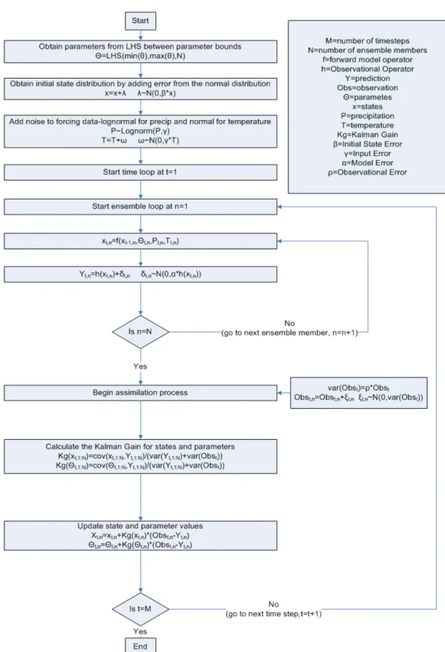
The Ensemble Kalman Filter (EnKF) is commonly used for hydrologic modeling applications. In hydrologic prediction, the EnKF is often used to update states but in this study the ability of the EnKF to estimate parameters is examined. The EnKF is an ensemble version of the Kalman Filter, performed as a Monte Carlo simulation, to overcome issues with applying the traditional Kalman Filter, including the need to linearize the model and to estimate the prior and posterior model error covariances for updating the model states. Supplementary to the description below, Figure 3 provides a descriptive flowchart of the EnKF. As the model progresses forward in time, the prior distribution of states is
, !, " #$% (4)
where is the forward operator (hydrologic model), represents the model predicted
(prior) states, represents the updated model states at the previous time-step, !
represents the meteorological forcing data, " represents the posterior model
parameters from the previous time-step, #$% is the model error, ' is the ensemble member
and is the time-step. Prior to update, an observational operator must be applied to the
states to bring them into the observation space, as in equation 5.
(′ ) * (5)
where (′ is the predicted observation and * is the observation error. Then the states
,
, +,-(. (′/ (6)
" " +01(. (′
2 (7)
where +, and +0 are the Kalman Gains for states and parameters respectively. The
Kalman Gain is calculated from:
+ 3454345 6 7,8788 6 (8)
Where 345 7,8 is the covariance of the states/parameter ensemble with the predicted
observation, HP;H< 788 is the variance of the predicted observations, and 6 is the
variance of the observational error in (8). H is the linearized observation operator
(4 =
,), which translates prior states from model space to measurement space. The
model state error covariance 3 can now be computed directly from the ensemble
deviations (>:
3
?@AB>
>
>
.?@AB C?D@AB (10)
+ 7,8788 7E (11)
4.2.2 Smoother
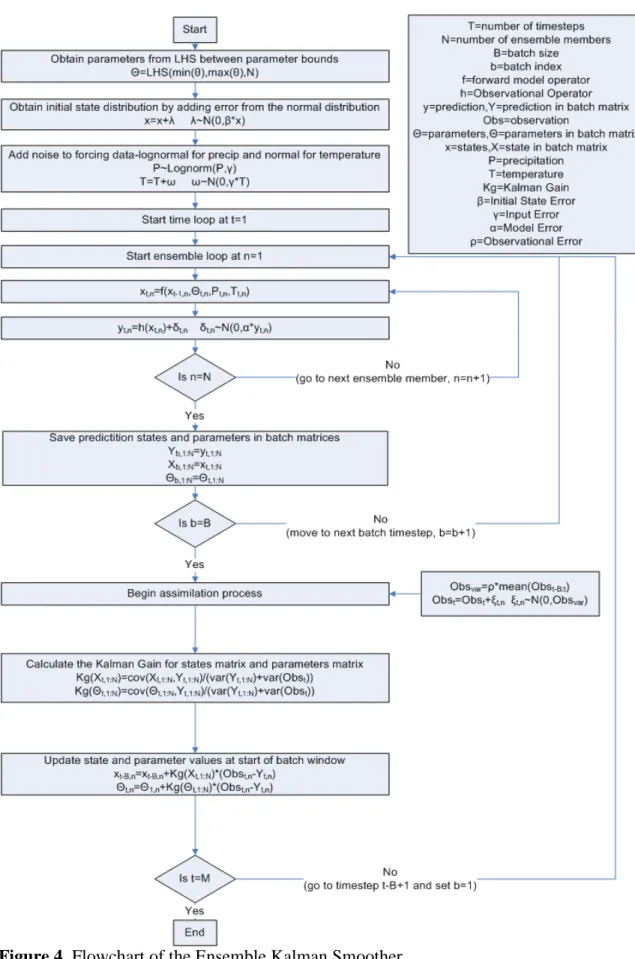
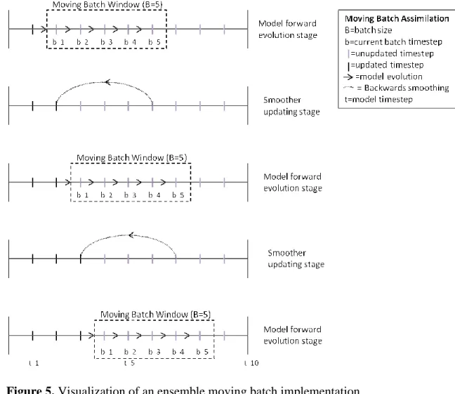
Each smoothing technique used in this study is implemented in a batch framework as outlined in [15] (see Figure 5). The EnKS performs the batch update the same as the EnKF in this application but instead of a single observation, multiple observations and predictions are applied in a vector in the Kalman gain equation. The observation and prediction vector is shown in 12 and 13.
( 1( (… (G25 (12)
(′′ -(′′ (′′… (′′′G/5 (13)
The states and parameters at each time-step are calculated according to Kalman Filter update equation. This calculation provides a state and parameter value for each time-step
in the sliding window. While it is clear that the model, beginning at time , should be
propagated forward with , the parameters, , must be set equal to the average over the
batch window, :I, as it is assumed that parameters are constant in this window. With
an updated ensemble of states and parameters, the batch window is moved forward one step and the process continues. This algorithm represented as a flowchart in Figure 4.
Figure 5. Visualization of an ensemble moving batch implementation
4.3Particle Filter
4.3.1 Filter
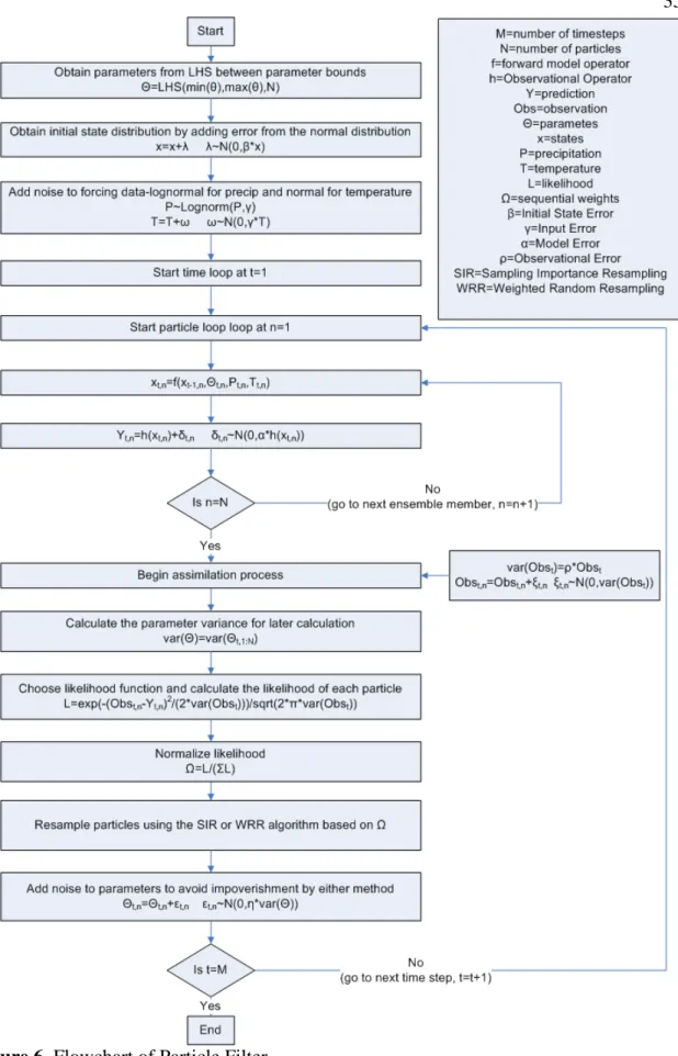
The PF, similar to the EnKF, sequentially calculates a posterior distribution of states and parameters. The advantage of the PF is, unlike the EnKF, it does not assume a Gaussian error structure, which allows the PF to more accurately predict the poste distribution. This is accomplished by resampling sets of state variables and parameters, or “particles”, with higher posterior weights, as opposed to the linear model state updating of the EnKF. Though this method is more accurate, it is more computa
Visualization of an ensemble moving batch implementation
The PF, similar to the EnKF, sequentially calculates a posterior distribution of states and parameters. The advantage of the PF is, unlike the EnKF, it does not assume a Gaussian error structure, which allows the PF to more accurately predict the poste distribution. This is accomplished by resampling sets of state variables and parameters, or “particles”, with higher posterior weights, as opposed to the linear model state updating of the EnKF. Though this method is more accurate, it is more computa
The PF, similar to the EnKF, sequentially calculates a posterior distribution of states and parameters. The advantage of the PF is, unlike the EnKF, it does not assume a Gaussian error structure, which allows the PF to more accurately predict the posterior distribution. This is accomplished by resampling sets of state variables and parameters, or “particles”, with higher posterior weights, as opposed to the linear model state updating of the EnKF. Though this method is more accurate, it is more computationally
demanding than the EnKF [49], The PF used in this study is the Sequential Importance Resampling (SIR) PF.
Based on the recursive Bayes Law (equation 14), the PF sequentially samples prior states and parameters to create an accurate posterior distribution, at each observation time-step.
J|L JMN,L T O8O8PP|,|,PPO,O,PP|Q|QPRSPRS, (14)
Equation 14 shows mathematically that a posterior conditional probability distribution of
model predicted states and parameters, () given all previous observations (L), can be
computed sequentially in time. It should be noted that all N in equation 14 are
observations as is signified in other equations by Q. Similar to the MCMC description
above, the probability of each particle in the PF is based on the likelihood equation. The sequential likelihood is calculated according to equation 15.
V(M , 2W ⁄ |61 Y| ⁄ exp ] . 1 26Y-(. (′/ ^ (15)
The normalized likelihood, J(M , , can easily be calculated by:
J(M , V(M , C V(?D_ M , J(. (′M6Y (16)
This probability is necessary to transform the prior particle weights into the posterior via equation 15. ` ` · J(M , C `· J(M , ?_ D (17)
In the SIR PF used in this study, prior particle weights, `, are set equal to 1/cO before
moving on to the next time-step. This results in a posterior weight, `, equal to
J(M , , the normalized likelihood. The SIR algorithm resamples those states
which have a probability greater than the uniform distribution. For further description of the resampling technique used refer to [33]. The PF algorithm is shown in flowchart form in Figure 6.
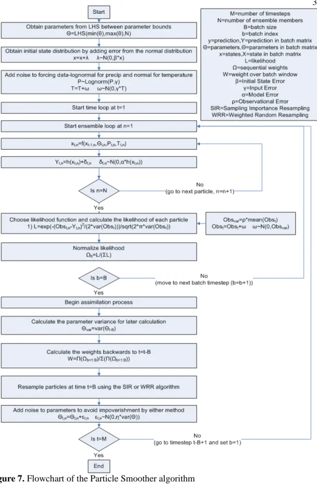
4.3.2 Smoother
The PF is extended to the PS by calculating a weight for each time-step in the sliding update window (see Figure 5), then resampling states and parameters at the beginning of the sliding window. This is performed by backward smoothing of particle weights. The formula for the backward smoothing of states is provided by [9, 27] and is presented in equation 18. This is then discretized in equation 19. This allows the weighting to be calculated based on multiple observations.
J|5 T J|5T O,O,PdSPdS|,|,POPOP|PP|P,,PP, P (18) J|5I ∑ J|5f Og,PdSh|,PAiOP|PA ∑ Og,PdSh |, P jiO P|Pj k jlS ? fD (19)
After applying equation 19 to calculate the weight at time , the particles are resample
using the SIR algorithm based on the weights at time . After resampling, the batch
window is moved forward one step and the process repeats. The PS algorithm is shown in flowchart form in Figure 7.
4.4Global Optimization via SCE-UA
In this study, Global Optimization is implemented using the SCE-UA algorithm [12-14]. This is a combination of the simplex gradient estimation technique and a Monte Carlo sampling to avoid convergence to a local optimum. This is performed by evolving multiple simplexes, which are referred to as a complex, and shuffling the estimates from separate simplexes within a complex after a certain number iterations. By shuffling the estimates within a complex, the possibility of convergence to a local optimum is reduced while increasing the speed of convergence. This method has been proven to be a robust method and therefore is used to estimate the optimal parameters.
4.5Markov Chain Monte Carlo Methods
MCMC techniques have become a popular method of hydrologic model calibration due to success in recent studies [3, 28, 30, 45, 46]. These studies showed that MCMC techniques can effectively calibrate hydrologic models and are becoming increasingly efficient. MCMC techniques are general methods for sampling a posterior
distribution. Through various sampling techniques, a proposal distribution O is created
based on the prior distribution mn. The probability W of a certain parameter set is
calculated according to the likelihood equation (20) assuming a non-informative prior distribution. Equation 20 is provided by [3] assuming homoscedastic and uncorrelated error.
W(| 2Wo/∏ >J q.-rPr′′P/s
ts u
In this equation, o is the variance, ( and (′′ represent the time-series of observed and
simulated data and is the number of observations. Equation 20 can be simplified by
integrating out the variance term giving equation 21 as described in [4, 45, 46].
W(| v∑ (D . (′′w
RP s
(21)
The probability of mn is compared to O in equation 22 to determine the x used in the
acceptance/rejection rule.
x y'z v {0_|r
{0|j}|r, 1w (22)
At each Markov Chain iteration, O is accepted/rejected if x is greater/less than a random
draw from the uniform distribution. After a sufficient number of chain iterations the model will converge to a stationary distribution. The assumption in this method, based on information presented in [32], is that this stationary distribution is the true posterior distribution. In order to determine if the model has converged to a stationary distribution, the variance of each Markov Chain is compared to variance of all Markov Chains as described by [21]. This statistic is assumed to show convergence when the value for all parameters is less than 1.2. This is because a value of 1, the perfect value, is very difficult and time consuming to achieve [21].
Currently, most hydrologic implementations of MCMC techniques are variants of the Metropolis Algorithm. The original Metropolis Algorithm is performed as a random walk to converge to the solution, making convergence of the algorithm very slow in complicated parameter spaces. Similar to how Monte Carlo techniques for optimization were improved through the addition of gradient approximations, the Metropolis
Algorithm has been improved with the use of adaptive search techniques. The Adaptive Metropolis, proposed by [23], has utilized the variance of the chains, at each iteration, to adapt the search area for each parameter based on new knowledge at each iteration. With the success of the Adaptive Metropolis, the Delayed Rejection Adaptive Metropolis [24] was presented. In addition to variance estimation of parameter predictions, genetic algorithms, such as Differential Evolution, have also been shown to be effective in minimizing the search area [5]. Separately these algorithms have been shown to be effective but in recent studies [46]. This is referred to as Differential Evolution Adaptive Metropolis (DREAM). The two techniques used in DREAM have been shown to be complimentary in some situations are capable of minimizing the number of chains necessary for convergence. Due to the efficiency and availability of the DREAM program, this algorithm is used to calibrate the hydrologic models in the comparison of global optimization, MCMC and filtering techniques.
5. Experimental Setup
This study is made up of two separate experiments. The first experiment examines the usefulness of remotely sensed microwave TB data assimilation on NWS operational models for the purpose of enhancing streamflow. The second study compares the effectiveness of Global Optimization, MCMC and data assimilation techniques for calibration of hydrologic models.
5.1Snow Data Assimilation Experiment
In the snow data assimilation portion of this study, the effects of microwave TB assimilation of prediction of SWE from the NWS SNOW-17 model and the streamflow from a the coupled SNOW-17 and SAC-SMA model are analyzed. The SWE estimation is compared in a synthetic experiment. A synthetic experiment was used because of the lack of an accurate validation dataset. This compares the effectiveness of the EnKF and the PF in estimation of SWE, using state only and joint state-parameter estimation. In the synthetic experiment the effectiveness of both methods is compared.
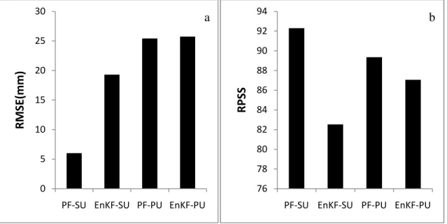
In order to determine the effectiveness of TB assimilation in the SNOW-17 model on streamflow prediction in the SAC-SMA model, six different experiments were run. Experiment 1 is a control run of both models to simulate the prediction in the current NWSRFC system. Experiment 2 is an ensemble run of both models, with the same input noise as the data assimilation experiments, without the implementation of data assimilation. Experiments 3-6 includes TB assimilation in the SNOW-17 model including (3) PF state estimation (PF-SU), (4) PF state-parameter estimation (PF-PU), (5) EnKF state estimation (EnKF-SU) and (6) EnKF state-parameter estimation (EnKF-PU). In
order to ensure consistency in comparing the assimilation techniques, all experiments use 1000 ensemble members, except for the PF-PU experiment which was raised to 3000 ensemble members to reduce the possibility of sample impoverishment. In addition to providing consistency between the methods, using the same ensemble size makes the computational cost of each method nearly exactly the same and thus computational cost will not be discussed in this study.
5.2Comparison of Calibration Techniques
Global Optimization, MCMC and data assimilation techniques are compared in this study to determine the relative benefits of each technique, in terms of calibration. The accuracy of all techniques will be compared with the Root Mean Square Error (RMSE) in a validation period, based on the average value at each prediction timestep for the ensemble assimilation methods. Each method is used to calibrate the HyMod and SAC-SMA models over a 10 year period. The models are then validated for the following 3 years.
5.3Performance Metrics
In the TB assimilation experiment, in order to determine the improvement of the assimilation experiments in relation to the control model run, the Benchmark Efficiency (BE) for streamflow prediction from each assimilation experiment is calculated. The BE is a measure of the improvement (if positive) over a simulation run. This is analogous to the Nash-Sutcliffe efficiency as the error is scaled by the control model run.
BE=1 .∑PlS~PPs
∑PlSPPs (23)
where AR is the assimilation run, O is the observation, CR is the control run and T is the total number of timesteps.
Ranked Probability Score is another widely used measure for evaluating the quality of probabilistic predictions [48]. By definition Rank Probability Score is the sum of squared error of the cumulative probability forecasts averaged over multiple events. In streamflow prediction, the probability forecast is usually expressed using a non-exceedance probability forecast within pre-specified categories (i.e., 5%, 10%, 25%, 50%, 75%, 90%, 95% and 99% non-exceedance). The observed value for a given threshold (forecast category) takes on the value of 1 if the observed flow value is less than the threshold for that category. Otherwise, the observed value is 0. The discrete expression of Rank Probability Score is given as:
63 C 1 D . 2
(24)
Where is the forecast probability at time t given by 3> )>) and
is the observed probability given by 3>*> )>)
where i is the
probability category. The Rank Probability Skill Score (RPSS) is also computed as the percentage improvement over a reference score (e.g. climatology)[48]:
63 ]1 .@^ 100 ]1 .
jhP|j|^ 100 (25)
Where 63nfmnm8 is the rank probability score for the observation. A positive