Multiple Imputation and Quantile Regression Methods for Biomarker Data subject to Detection Limits

(1)

MULTIPLE IMPUTATION AND QUANTILE

REGRESSION METHODS FOR BIOMARKER

DATA SUBJECT TO DETECTION LIMITS

by

MinJae Lee

BS in Statistics, Sookmyung Women’s University, Korea, 2000

BS in Computer Science, Sookmyung Women’s University, Korea,

2000

MS in Statistics, Sookmyung Women’s University, Korea, 2004

Submitted to the Graduate Faculty of

the Department of Biostatistics in partial fulfillment

of the requirements for the degree of

Doctor of Philosophy

University of Pittsburgh

2010

(2)

UNIVERSITY OF PITTSBURGH DEPARTMENT OF BIOSTATISTICS

This dissertation was presented by

MinJae Lee

It was defended on August 31, 2010 and approved by

Lan Kong, Ph.D., Assistant Professor,

Department of Biostatistics, Graduate School of Public Health, University of Pittsburgh

Lisa Weissfeld, Ph.D., Professor,

Jong-Hyeon Jeong, Ph.D., Associate Professor,

Sachin Yende, M.D., M.S., Assistant Professor,

Department of Critical Care Medicine, School of Medicine, University of Pittsburgh Dissertation Director: Lan Kong, Ph.D., Assistant Professor,

(3)

Copyright c by MinJae Lee 2010

(4)

MULTIPLE IMPUTATION AND QUANTILE REGRESSION METHODS FOR BIOMARKER DATA SUBJECT TO DETECTION LIMITS

MinJae Lee, PhD University of Pittsburgh, 2010

Biomarkers are increasingly used in biomedical studies to better understand the natural his-tory and development of a disease, identify the patients at high-risk and guide the therapeutic strategies for intervention. However, the measurement of these markers is often limited by the sensitivity of the given assay, resulting in data that are censored either at the lower limit or upper limit of detection. Ignoring censoring issue in any analysis may lead to the biased results.

For a regression analysis where multiple censored biomarkers are included as predictors, we develop multiple imputation methods based on Gibbs sampling approach. The simula-tion study shows that our method significantly reduces the estimasimula-tion bias as compared to the other simple imputation methods when the correlation between markers is high or the censoring proportion is high.

The likelihood based mean regression for repeatedly measured biomarkers often assume a multivariate normal distribution that may not hold for biomarker data even after trans-formations. We consider a robust alternative, median regression, for censored longitudinal data. We develop an estimating equation approach that can incorporate the serial corre-lations between repeated measurements. We conduct simulation studies to evaluate the proposed estimators and compare median regression model with the mixed models under various specifications of distributions and covariance structures.

Missing data is a common problem with longitudinal study. Under the assumptions that the missing pattern is monotonic and the missingness may only depend on the observed data,

(5)

we propose a weighted estimating equation approach for the censored quantile regression models. The contribution of each individual to the estimating equation is weighted by the inverse probability of dropout at the given occasion. The resultant regression estimators are consistent when the dropout process is correctly specified. The performance of our estimating procedure is evaluated via simulation study.

We illustrate all the proposed methods using the biomarker data of the Genetic and Inflammatory Markers of Sepsis (GenIMS) study. Appropriate handling of censored data in biomarker analysis is of public health importance because it will improve the understanding of the biological mechanisms of the underlying disease and aid in the successful development of future effective treatments.

Keywords: Left-censored data; Detection limits; Multiple imputation; Gibbs sampler; Me-dian regression; Quantile regression; Longitudinal data; Drop-out.

(6)

TABLE OF CONTENTS

1.0 INTRODUCTION . . . 1

2.0 LITERATURE REVIEW. . . 6

2.1 Statistical Methods for Missing Data . . . 7

2.1.1 Missing Covariates . . . 7

2.1.2 Missing Response Variables . . . 8

2.2 Existing Methods for Left-Censoring Data . . . 9

2.2.1 Naive and Imputation Approaches . . . 9

2.2.2 Likelihood Based Approaches . . . 10

2.2.3 Quantile Regression Approaches . . . 11

2.3 Analysis of Longitudinal Data with Dropouts . . . 12

2.3.1 Likelihood Based Approaches . . . 12

2.3.2 Weighting Techniques for Quantile Regression Approaches . . . 13

3.0 MULTIPLE IMPUTATION APPROACHES FOR THE CENSORED COVARIATES . . . 15

3.1 Introduction . . . 15

3.2 Notation and Methods . . . 18

3.2.1 Multiple Imputation For Single Censored Marker . . . 19

3.2.2 Multiple Imputation For Multiple Censored Markers . . . 21

3.3 Simulation Study . . . 23

3.4 Application . . . 26

(7)

4.0 MEDIAN REGRESSION FOR LONGITUDINAL LEFT-CENSORED

RESPONSES . . . 30

4.2.1 Censored Median Regression . . . 32

4.2.2 Weighted Censored Median Regression . . . 34

4.5 Discussion . . . 42

5.0 QUANTILE REGRESSION FOR LONGITUDINAL BIOMARKER DATA SUBJECT TO LEFT CENSORING AND DROPOUTS . . . 44

5.2.1 Censored Quantile Regression . . . 46

5.2.2 Censored Quantile Regression accounting for dropouts . . . 48

5.5 Discussion . . . 57

6.0 CONCLUSION AND DISCUSSION . . . 58

(8)

LIST OF TABLES

1 Simulation Results of Multiple Imputation for One Marker at a Time. . . 24

2 Simulation Results of Multiple Imputation for Higher Correlated Markers . . 26

3 Analysis Results for Prediction of AKI using Day 1 Cytokines and Fibrinolysis Markers . . . 28

4 Simulation Results of Censored Median Regression . . . 38

5 Simulation Results Comparing Censored Median Regression with Tobit Mixed Model . . . 39

6 Longitudinal Analysis of GenIMS IL6 vs Severe Sepsis . . . 41

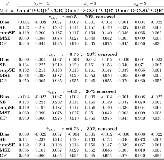
7 Simulation Results of Censored Quantile Regression accounting for Dropout . 52

8 Estimation Results for Missing Data Model . . . 55

(9)

LIST OF FIGURES

1 Daily Censoring Proportions of GenIMS Cytokines in the 1st week of

Hospi-talization . . . 3

2 Mean and Median Regression Results for GenIMS Cytokine IL6. . . 42

3 Histogram of IL6 and ln(IL6) . . . 54

(10)

1.0 INTRODUCTION

Biomarkers are increasingly used in biomedical studies for diagnosis and prognosis of acute and chronic diseases, gaining insight of treatment effectiveness and establishing the potential disease pathways to guide the future treatment targets. The accuracy of biomarker measure-ments is very important for making valid and reliable conclusions of the findings. However, the biomarker data are subject to various sources of measurement errors. This includes error associated with specimen collection, processing, and storage; laboratory error (both within and between batches); and variability in the biomarker levels over time within an individual. Left-censoring, which is due to the limits of detection (LOD), is also a common source of error that may not be noticed in the analysis stage of biomarker data. LOD is the lowest concentration of analyte in a sample that can be detected under the stated experi-mental conditions. Reportable or quantifiable measurements are only those above LOD. For example, left-censoring occurs in the assessment of viral RNA in patients infected with the human immunodeficiency virus (HIV) (Hughes [29]) , antibody concentration in blood serum (Moulton et al. [46]), and the interleukin-10 (IL10) and IL6 in community-acquired pneu-monia (CAP) patients (Kellum et al. [35]). Despite the improvement in assay sensitivity, left-censoring remains a critical issue in some studies because the ultra sensitive assays may be too expensive to use in a large cohort study or the biomarker concentrations are much lower than expected. Left-censoring problem results in many challenges in the statistical analysis of biomarker data. Ignoring the censored observations or replacing them with an arbitrary constant will introduce biased results in the analysis. It is imperative to develop statistical methods to address this issue appropriately and efficiently.

We encountered the left-censoring data from an inception cohort study of sepsis: the Genetic and Inflammatory Markers of Sepsis (GenIMS) study [35]. GenIMS study is a

(11)

multicenter study of 2320 subjects from the emergency department (ED) with community-acquired pneumonia (CAP), the most common cause of sepsis. It was coordinated by the CRISMA Laboratory, Department of Critical Care Medicine at the University of Pittsburgh between 2001 and 2003. Sepsis is the leading cause of death in critically ill patients in the United States (Hotchkiss et al. [54]). Sepsis is defined as a systemic inflammatory response syndrome that occurs during infection (Bone et al. [7]). The frequency of sepsis is expected to increase given an aging population and increasing number of patients with chronic treatment-resistant infections. Better understanding of the pathophysiology of sepsis from the inflammatory, procoagulant and immunosuppressive aspects has contributed to the emergence of several therapeutic plans (Russell [59]). The treatments can be very effective if applied expeditiously, however rapid diagnosis of sepsis remains to be difficult. Many people are pressing to identify the important biomarkers for risk prediction of sepsis and the subsequent adverse outcomes. Meanwhile, gaining more insights of the roles of different pathways through more sophisticated modeling may reveal novel targets and new mechanisms of action that help to improve the current treatment. The main goals of GenIMS study are to better understand the natural history and development of sepsis, and to identify the biomarkers indicating the risk for severe sepsis, multiple organ failure, and death. A set of inflammatory and coagulation markers were evaluated repeatedly during the course of hospitalization. However, the assays used were not sensitive enough to measure low concentrations of some biomarkers, resulting in heavy left-censoring data. Figure 1presents the censoring proportion of cytokines (TNF (tumor necrosis factor), IL6 (interleukin-6) and IL10) over the first seven days. Since left-censoring introduces informative missing data that are not ignorable, the traditional regression analyses are no longer valid.

The ad-hoc methods using either the LOD, or some other arbitrary value such as the LOD/2, or the LOD/√2, usually lead to biased results towards null. The simple ”fill-in” imputation approaches based on certain distributional assumptions of the data eliminate the bias when the censoring is moderate (<30%), but introduce the biased variance estimates. The multiple imputation approaches can often provide valid statistical inference when the censoring proportion is not high (< 50%) [32]. Although these simple methods have lim-itations, they are easy to use in practice when censored biomarkers are either considered

(12)

Figure 1: Daily Censoring Proportions of GenIMS Cytokines in the 1st week of Hospitaliza-tion

as predictors or dependent variables, also they aid in the graphic display of the raw data. More efficient statistical models have also been developed for handling the left-censoring data. To accommodate single censored covariates, Lynn [43] presented the likelihood-based approaches for linear and logistic models; Rigobon and Stoker [52] proposed a two-part re-gression model for both parametric and semiparametric models, where an index model was used to estimate the censored covariates. The same idea was adopted by D’Angelo and Weissfeld [10] to handle the censored covariates in the Cox model.

Much of the work for left-censored data has focused on censored response variables. The likelihood based approaches requires specification of the distribution of the response variables. The regression parameters can be estimated by maximizing a likelihood function contributed by both observed and censored observations. For example, the Normal distri-bution is assumed in the Tobit linear regression model (Tobin [72]) and mixed models for longitudinal censored data (Hughes [29]; Lyles et al. [42]; Jacqmin-Gadda et al. [31]; Wu [75]; Thiebaut et al. [70]). However the biomarker data are often highly skewed, even af-ter log transformation. In this case, the quantile regression (QR) is more attractive than

(13)

the least squares regression or any likelihood based method. Without imposing a full dis-tribution on the response variable, QR provides a robust alternative and also allows one to look at covariate effects on various quantiles of a response variable. Most work on QR was done for independent data in econometrics. Powell [50] first considered the least ab-solute deviations (LAD) estimation which leads to the median regression estimator. LAD estimation method was later extended to more general quantiles (Powell [51]). Little work has been done for dependent observations until recently when Wang and Fygenson [73] pro-posed an inference procedure for longitudinal studies with application to a HIV/AIDS study.

As multiple biomarkers were measured over time from different potential pathways in Gen-IMS study, left-censoring data from multiple markers results in many new challenges in statistical analysis. This dissertation will focus on the following three statistical issues:

1. Multiple Censored Predictors

In order to identify the important predictors of sepsis or mortality at 90 days, multiple cytokine and coagulation markers along with clinical predictors are considered in the logistic regression model. However, while several markers had various amounts of cen-soring data, the existing methods are difficult to use due to computational intensity. We will propose a multiple imputation (MI) approach for this problem that can account for the correlations between markers. Our approach is based on the use of Tobit regression and Gibbs sampling.

2. Longitudinal Censored Responses

Mixed models and GEE methods are two popular approaches for analyzing longitudinal data. But only mixed models have been extended for the left-censoring responses as mentioned earlier. Mixed models may lead to biased results when the covariance struc-ture of responses is misspecified. GEE methods overcome this problem, but require data to be missing completely at random. This is a stronger assumption than that required for the mixed model. The QR model is close to the GEE approach in that the estimating equations are formed to obtain the regression coefficient estimators and both are robust

(14)

to misspecification of variance structure. Extending the approach of Wang and Fygenson [73], we will develop the estimating procedures to modeling the censored marker data while accounting for serial correlations between repeated measurements.

3. Missing Data due to Dropouts

The biomarker data of GenIMS study were collected during the course of hospitalization. The missing data arose due to death or discharge early and administrative errors. The dominant missing pattern is monotone missing associated with dropout. The dropouts here refer to the cases that the patients had marker measurements up to a certain day and then no more measurements were collected afterwards because they were discharged early or died in the hospital. In GenIMS study, the subjects who had a lower level of IL6 appeared more likely to drop out. The inverse probability weighed GEE approach of Robins et al. [53] has been commonly used to handle the informative missing data for mean regression models. Assuming monotone missing data patterns and MAR mecha-nism, Lipsitz et al. [36] and Yi and He [77] adopted this approach to quantile regression models for uncensored data. The basic idea of this approach is that an individual’s con-tribution to the traditional estimating equations is weighted by the inverse probability of dropout at the given occasion. We will apply the same weighting technique to the censored quantile regression estimating equation.

The organization of this dissertation is as follows. First, we review the literature work on missing data problem, existing methods for left-censored data and quantile regression methods in Chapter 2. Then we propose statistical methods to address the above three issues. In chapter 3, we present the multiple imputation methods based on gibbs sampling for multiple censored predictors. In chapter 4, we develop the median regression model to handle the left-censored longitudinal responses. In chapter 5, we propose the weighted censored quantile regression to incorporate the missing data due to dropouts. In chapter 6, we summarize the dissertation work and discuss some future work.

(15)

2.0 LITERATURE REVIEW

Left-censoring data is a special form of missing data. Rubin and Little [39] developed a terminology for different missing values processes. Three missing data mechanisms defined by Little and Rubin are: MCAR (missing completely at random), MAR (missing at random), and NMAR (not missing at random). There are several reasons why the data may be missing; they may be missing because equipment malfunctioned, the weather was terrible, or people got sick, or the data were not entered correctly. When we say that data are missing completely at random, we mean that the probability that an observation (Xi) is missing is unrelated to the value of Xi or to the value of any other variables. Often data are not missing completely at random, but they may be classifiable as missing at random (MAR). The data can be considered as missing at random if the data meet the requirement that missingness does not depend on the value ofXi after controlling for another variable. If data are not missing at random or completely at random then they are classed as Not Missing at Random (NMAR). For example, if we are studying mental health and people who have been diagnosed as depressed are less likely than others to report their mental status, the data are not missing at random. Left-censoring data due to LOD are non-ignorable missing data, i.e., NMAR. Usually the statistical inference for NMAR data is complicated and the knowledge of missing mechanism is critical for valid estimation and inference. Left-censoring is a fixed censoring that is different from random censoring as seen in the survival analysis. The missing mechanism is clearly known and thus the modeling is less difficult than the general NMAR setup. The statistical framework for handling missing data can be adopted to left-censoring data with appropriate adjustment. In this chapter, we will first describe some methods to handle NMAR data in missing data literature, then we will review the existing methods for left-censoring data including naive approaches and efficient statistical

(16)

approaches. We will also discuss briefly the statistical methods for handling missing data due to dropouts.

2.1 STATISTICAL METHODS FOR MISSING DATA

Statistical inference from missing data has been a researched topic over the last two decades. Since most statistical methods were derived for fully observed data, the impact of missing values is an issue. Missing values can occur on response variables (outcomes) and on covari-ates (predictors). The goal of a statistician still remains the same with or without missing values and they are required to draw valid and efficient inferences about its population of interest. Rubin and Little [59] developed a terminology for different missing values processes. Three missing data mechanisms defined by Little and Rubin are: MCAR, MAR, and NMAR. In this study, we focus on the methods for NMAR data.

2.1.1 Missing Covariates

Rubin [57] developed a framework of inference from missing data that remains in use today. There are the approaches for the missing covariates in regression models (Little, JASA [38]) and Little [37] provided a review of methods that can handle missing covariates into six classes. The first class is the complete-case (CC) analysis and the second is the available-case (AC) methods. Available-available-case analysis approaches use the largest sets of available available-cases for each of parameters (Little and Rubin [39]). The problem of this AC analysis is that the estimated covariance matrix of theX’s is not necessarily positive definite, which leads to in-ferior results compared to CC analysis for highly correlated data (Haitovsky [22]). The third method discussed by Little includes Lest Squares (LS) on imputed data methods. In this setting, the missing covariates are imputed and a regression of response variable on covariates is performed on the filled in data by ordinary least squares or weighted least squares regres-sion. The imputation methods were unconditional and conditional mean imputation. The inference based on these methods lead to the biased and imprecise results. The fourth class is

(17)

the class of maximum likelihood (ML) methods. In this method, a classical ML estimate for a model for the joint distribution ofY and X would be the multivariate normal with meanµ

and covariance matrix Σ. Another method would be Expectation Maximization (EM) algo-rithm. The EM algorithm (Dempster, Laird and Rubin [12]) is a general iterative algorithm for ML estimation in data with missing values. The EM algorithm consists of Expectation (E-step) and Maximization (M-step). The E-step provides the conditional expectation of the complete data log-likelihood given the observed data and current estimated parameters and then substitutes these expectations for the missing data. In the M-step, we can have a maximum likelihood estimation of the parameters as if there were no missing data. The M-step gives the parameter estimates to maximize the complete data log-likelihood from the E-step. The fifth class in Little’s paper was the Bayesian methods. In Bayesian inference, information about unknown parameters is expressed in the form of a posterior distribution. Markov Chain Monte Carlo (MCMC) has been applied as a method for exploring posterior distributions in Bayesian inference. In MCMC, one constructs a Markov chain long enough for the distribution of the elements to stabilize to a common, stationary distribution. By repeatedly simulating steps of the chain, it simulates draws from the distribution of inter-est. The last class considered by Little has the multiple imputation (MI) methods. Rubin [58] introduced the idea of MI in which each missing value is replaced with M times using simulated values prior to analysis. This will produce M possible complete datasets that are the analyzed in the same manner as a complete dataset. For the inference, these results are then combined by simple arithmetic to obtain overall estimates along with their standard errors that reflect missing data uncertainty as well as the sample variation.

2.1.2 Missing Response Variables

If the probability of missingness is associated with the unobserved response values that should have been obtained, the missing data mechanism is said to be not missing at random (NMAR). This process is often referred to as non-ignorable missingness due to the fact that the missing data mechanism must be considered to make a valid inference about the distribution of the responses (Little and Rubin [40]; Fitzmaurice et al. [17]; Allison [1]). In a

(18)

longitudinal study the term dropout refers to the situation where a response at a particular time being missing, implies that all the subsequent follow-up responses are also missing (Fitzmaurice et al. [17]; Little and Rubin [40]). In this scenario, the standard likelihoods for analyzing longitudinal biomarker data do not include a mechanism for incorporating different reasons for loss to follow-up or death. When the measurements are missing due to dropout or death, the two types of loss to follow-up are different and should not be combined (Dufouil et al. [13]). In the full data modeling setting every observation is equally weighted. For modeling data with missing observations, weighting techniques have been used for semi-parametric regression modeling (Robins et al. [53]). The weighting procedure has been applied in analyzing many incompleted longitudinal data problems by Rotnitzky and Robins [55], Lipsitz et al. [36], Lin, Demirtas [11], Dufouil et al. [13], Ibrahim et al. [30]. Weights are computed by inverting the probabilities of response. In a longitudinal study some subjects are more likely to complete the study than others. The pseudo-likelihood approach has been used for estimating parameters in generalized linear mixed models (Wolfinger and O’connell [74]) and also non-ignorable missing covariate in cox model was proposed by Herring and Ibrahim [26].

2.2 EXISTING METHODS FOR LEFT-CENSORING DATA

Several approaches have been proposed in the statistics literature for the analysis of lon-gitudinal left-censored data and all approaches differ in sophistication when handling the truncated values.

2.2.1 Naive and Imputation Approaches

Naive approaches are to use only observed data or replace censored observations with a single value i.e., Limit of Detection (LOD) (Keet et al. [34]), LOD/2 or LOD/√2 (O’Brien et al.; Hornung and Reed [28]). If the distribution of the measurement data is known, then an alternative strategy replaces values below the detection limit with expected values of the

(19)

missing measurements, conditional on being less than the detection limit (Garland et al. [18]; Gleit [21]). Calculation of the conditional expected value requires the investigator to either know or estimate parameters of the measurement distribution. The substitution schemes are simple but because a single value represents all measurements below the detection limit, parameter estimates and their variances are likely biased. this limitation led to a single-impute ”fill-in” method (Helsel [25]; Moschandreas et al. [44, 45]). An investigator first characterizes the form of the distribution and estimates its parameters and then assigns randomly sampled values below the detection limit from the estimated distribution. Fill-in values along with measured values above the detection limit are then used in analyses. The fill-in method did not include complex modeling of regression factors. In addition, although the fill-in approach assigned random values from an appropriate distribution, it did not account for the variability of the imputation process, because the inserted values are not real data. For the imputation of the values of the detection limit, single imputation and multiple imputation (Lubin et al. [32]; De Roos et al. [4]) have been considered. Because different methods are needed to handle censored dependent variables and censored covariates, there are different approaches for these cases.

2.2.2 Likelihood Based Approaches

Especially, for the censored dependent variables, there are many likelihood based approaches where the distribution is fully specified. A standard method for the analysis of censored data is Tobit regression. Tobit regression based on normal assumption (Gilbert [20]; Persson & Rootzen [49]; Tobin [72]). Tobit regression has been extended to multivariate regression (Amemiya [2]). Recently a Box-Cox transformation has been used for the analysis of left-censored cross sectional data (Han and Kronmal [23]). Linkage analysis of left-censored trait data has been based on the variance component of the Tobit model (Epstein et al. [15]). In this model, the traditional variance component model has been modified to accommo-date the censored data by random effects. The mixed models for the longitudinal censored data have been proposed. Hughes [29] modified the usual EM estimation procedure for the mixed effects model to account for left-censoring. The method uses Monte Carlo procedure

(20)

to provide a general solution can be used with left-censored data and since the expectation step of the EM algorithm is intractable, the Gibbs sampler is used to implement a Monte Carlo expectation step in the EM algorithm. Jacqmin-Gadda et al. [31] proposed an ap-proach of direct maximization of the likelihood without the EM or the Monte Carlo methods where maximization is based on the Marquardt algorithm. The Lyles et al. [42] approach was based on a hierarchical formulation of the likelihood, and estimation was carried out by direct maximization of the likelihood using built-in algorithms. Lyles et al. [42] ana-lyzed left-censored longitudinal data with informative dropout HIV data by maximizing a single likelihood function which has integrated the censoring and informative dropout pro-cess. They estimated the parameters from this complicated likelihood function and compute the standard errors using the observed information matrix directly. Thiebaut et al. [70] considered joint modeling for bivariate longitudinal data. To accommodate single censored covariates, Lynn [43] presented the likelihood-based approaches for linear and logistic mod-els, two-step linear regression model with index model used to estimate censored/selected covariates (Rigobon and Stoker [52]) and left-censored covariates in cox model (D’Angelo and Weissfeld [10]) have been proposed. There are many issues in analyzing left-censored longitudinal data using a full likelihood. Beyond the algebraic and numeric intractability, it requires computation of a series of multiple integrals and becomes intractable for the case of a high rate of censoring.

2.2.3 Quantile Regression Approaches

In addition to these likelihood based approaches, the quantile regression approaches have been developed for left-censoring data. The quantile regression (QR) methods have been well developed for independent and longitudinal data when there is no censoring issue. For fixed censoring, i.e., the observations are censored at a fixed constant, and most work on QR was done for independent data in econometrics. Powell [50] first considered the least absolute deviations (LAD) estimation which lead to the median regression estimator. LAD estimation method was later extended to more general quantiles [51]. The censored quantile regression is very appealing for analyzing economic data due to its robustness to

(21)

nonnor-mality or heteroscedasticity. However, the computation of censored QR estimators and associated variance estimators is challenging because the objective function is not convex and an unknown density function needs to be estimated.

No work has been done for dependent observations until recently Wang and Fygenson [73] proposed an inference procedure for longitudinal studies with application to a HIV/AIDS study. A simple quantile rank score test was developed to test for the treatment effect, while the regression coefficient of treatment effect was not directly estimated. This approach avoided the computation of the complex variance estimator. In the observational study like GenIMS, the point estimates of all the covariate effects are of equal importance. The meth-ods focusing on the estimating procedures are not fully developed yet.

2.3 ANALYSIS OF LONGITUDINAL DATA WITH DROPOUTS

2.3.1 Likelihood Based Approaches

We often encounter missing data due to dropouts in longitudinal studies. Generalized esti-mating equations (GEEs) can be used for estiesti-mating the parameters of marginal models in longitudinal studies and provide consistent estimates when the missingness is independent of both the observed and missing data (MCAR). If missingness may be related to the ob-served responses but conditionally independent of the missing data (MAR), GEE methods are no longer valid. However, mixed models can handle data that are MAR. When there are missing data that are not ignorable (NMAR), mixed models will result in biased estimates. For general missing patterns, the selection model and mixture model are commonly used for modeling non-ignorable missing longitudinal data. The selection model is based on the joint distribution which is a product of the complete data model. The interest of the selection model is in parameter which is under the hypothesized complete data. If the full data is modeled as a mixture over dropout categories then it is called a pattern mixture model. In the pattern mixture model, the parameter conditional on the missing data pattern is the

(22)

primary interest. These models are under-identified and well suited for small percentages of missing observations.

If data are missing due to dropout, joint modeling is a common strategy to handle infor-mative dropout data (NMAR). Such models have been considered for longitudinal censored data. Lyles [42] implemented a maximum likelihood procedure to estimate initial HIV RNA levels and slopes within a population, compare these parameters across subgroups of HIV-infected women and illustrate the importance of appropriate treatment of left-censoring and informative dropouts. Thiebaut [70] propose a likelihood inference for a parametric joint model including a bivariate linear mixed model for the two markers and a log normal sur-vival model for the time to dropout. Gao and Thiebaut [66] considered the situation when the longitudinal outcomes are also subject to non-ignorable missing in addition to truncation. A shared random effect parameter model is presented where the missing data mechanism depends on the random effects used to model the longitudinal outcomes.

The weighting techniques have been considered for semi-parametric regression modeling (Robins et al. [53]) and has been applied in analyzing many incomplete longitudinal data problems by Rotnitzky and Robins [55], Lipsitz et al. [36], Demirtas [11], Dufouil et al. [13], Lin et al. [27] and Ibrahim et al. [30]. Weights are computed by inverting the probabilities of being observed. In the longitudinal study, some subjects are more likely to complete the study than others. The pseudo-likelihood approach has been used for estimating parameters in generalized linear mixed models (Wolfinger and O’connell [74]).

2.3.2 Weighting Techniques for Quantile Regression Approaches

Like the GEE method, standard estimating functions of quantile regression models result in consistent estimators when the data are missing completely at random. For missing data due to dropouts and under MAR mechanisms, Lipsitz et al. [36] and Yi and He [77] adopted the inverse probability weighted GEE approach to quantile regression models for uncensored data. Lipsitz et al. [36] mainly focused on the application of quantile regression methods using the independent working assumption of covariance structure to longitudinal responses with dropout and discussed methods for estimating the parameters of marginal models, in

(23)

which the median or any other quantile of an individual’s response at timet is modeled as a function of a time trend and a set of covariates. Yi and He [77] considered median regression models to analyze a longitudinal data set arising from a controlled trial of HIV disease and they incorporated the covariance structure in the estimation procedures and established the asymptotic properties for the resultant estimators. The basic idea of this weighting approach is that an individual’s contribution to the traditional estimating equations is weighted by the inverse probability of dropout at the given occasion, i.e., the conventional estimating equations for the quantile regression parameters are weighted inversely proportionally to the probability of dropout. This approach requires the process generating the missing data to be estimable but makes no assumptions about the distribution of the responses other than those imposed by the quantile regression model. This method yields consistent estimates of the quantile regression parameters provided that the model for dropout has been correctly specified. There are many ways to handle informative dropouts in the mixed models or GEE approaches when data are not censored, but limited work was done for quantile regression models [36, 76]. Lyles et al. [42] and Thiebaut et al. [70] studied the mixed models for left-censoring data with informative dropouts. The corresponding method for QR is still lacking.

(24)

3.0 MULTIPLE IMPUTATION APPROACHES FOR THE CENSORED COVARIATES

Increasingly used in biomedical studies for the diagnosis and prognosis of acute and chronic diseases, biomarkers provide insight into the effectiveness of treatments and potential path-ways that can be used to guide future treatment targets. The measurement of these markers is often limited by the sensitivity of the given assay, resulting in data that are censored either at the lower or upper limit of detection. For the Genetic and Inflammatory Markers of Sepsis (GenIMS) study, many different biomarkers were measured to examine the effect of different pathways on the development of sepsis. In this study, the left-censoring of several important inflammatory markers has led to the need for statistical methods that can incorporate this censoring into any analysis of the biomarker data. This paper focuses on the development of multiple imputation (MI) methods for the inclusion of multiple left-censored biomarkers in a logistic regression analysis. A multivariate normal distribution is assumed to account for the correlations between biomarkers. The Gibbs sampler is used for estimation of the dis-tributional parameters and imputation of the censored markers. The proposed methods are evaluated and compared with some simple imputation methods through simulation. A data set of inflammatory and coagulation markers from the GenIMS study is used for illustration.

3.1 INTRODUCTION

Biomarkers are now a key component of many biomedical studies, providing insight into potential treatment targets and disease pathways. They also provide key information that can be used to inform the diagnosis and prognosis of both acute and chronic diseases. While

(25)

biomarkers provide useful information, they are also subject to many different limitations due to numerous sources of measurement errors and difficulty in collecting the actual speci-mens. In addition to the error associated with specimen collecting/processing and laboratory error, left-censoring due to the limits of detection (LOD) is also a common source of error that needs to be addressed at the analysis stage of biomarker data. Left-censoring can be addressed through the use of assays that are more sensitive; however, this is often not feasible due to the cost and time constraints of many studies. Well-known examples of left-censoring occur in the assessment of viral RNA in patients infected with the human immunodeficiency virus (HIV) [29], the antibody response to vaccine in blood serum [46], and the biomarkers interleukin-10 (IL10) and interleukin-6 (IL6) that were collected in the Genetic and Inflammatory Markers of Sepsis (GenIMS) study [35]. In the GenIMS study, the motivating example for this work, a set of inflammatory and coagulation markers were evaluated repeatedly during the course of hospitalization. These markers were measured daily during the first week of hospitalization and less frequently after day 7. The assays used to measure the concentration of the biomarkers in GenIMS were not sensitive enough to detect levels of the molecule at the low end of normal, resulting in moderate to heavy left-censoring of the biomarker data. Since left-censoring generates informative missing data that are not ignorable, the traditional methods of statistical analysis are not optimal and may be invalid. Thus statistical methods that can be applied to left-censored biomarker data are needed.

One common approach that has been applied to the analysis of left-censored data is the use of ”fill-in” methods where the left-censored observation is replaced by the LOD, the LOD/2, or the LOD/√2 depending on the assumed shape of the left tail of the distribu-tion. This approach is straightforward to implement, but leads to results that are biased towards the null hypothesis. The simple ”fill-in” imputation approaches based on certain distributional assumptions of the data eliminate this bias when the censoring is moderate (< 30%), but introduce bias into the associated variance estimates. Multiple imputation (MI) approaches [58] are useful and provide valid statistical inference when the censoring proportion is not high (< 50%) [32]. The ”fill-in” methods have some limitations but easy to use in practice and apply to either the outcome or the predictor in an analysis.

(26)

Most of methodological development for censored biomarkers has focused on the case where the biomarker is considered as the outcome variable. One commonly applied model for this setting is the Tobit linear regression model [72,49]. This model has been extended to include a variance component model for the analysis of clustered left-censored outcome data [15]. Many other researchers have developed mixed models for longitudinal left-censored data [29, 31, 42, 75, 70]. For non-normal left-censored outcome data, a method based on the Box-Cox transformation has been proposed by Han and Kronmal [23]. Lyles et al. [41] focused on the estimation of the correlation coefficient when the data are left-censored.

There have been fewer proposals for methods that accommodate censored predictors. Lynn [43] developed likelihood-based methods that can be applied to linear and logistic models with a single censored covariate. Austin and Hoch [5] compared several approaches for censored covariates in a simulation study that was designed to evaluate the bias of estimates for a censored covariate in a linear regression model. Rigobon and Stoker [52] proposed a two-part regression model for both parametric and semi-parametric models, where an index model was used to estimate the censored covariates. The same idea was adopted by D’Angelo and Weissfeld [10] to handle censored covariates in the Cox model. The methods discussed above can be very useful for modeling when only one covariate is censored, but are not easily extended to the multiple covariate setting where the covariates may be correlated. As a result, there are no methods that are available for the inclusion of multiple censored covariates in a regression model.

The focus of this work is on the development and evaluation of potential methods for the setting of multiple censored covariates in a regression model. We propose the use of multiple imputations (MI) due to its simplicity and the fact that it has been shown to be a competitor to maximum likelihood method [43]. A simple MI approach has been used by De Roos et al. [4] to estimate the risk of non-Hodgkin’s lymphoma associated with the level of organochlorine chemicals in plasma. However, they assumed a univariate distribution for each censored predictor without accounting for the potential correlation between predictors. The motivation for this work comes from the analysis of biomarker data collected in the GenIMS study, where multiple biomarkers of interest are measured with many of these biomarkers being left-censored. The analysis is similar to that of De Roos et al. [4] with the

(27)

focus being the prediction of acute kidney injury (AKI) as a function of several, potentially correlated biomarkers. Thus we propose the use of MI methods that account for the potential correlation of the biomarkers by assuming a multivariate normal distribution. The method is based on the use of a Tobit regression model combined with a Gibbs sampler to estimate the distributional parameters and to impute the censored covariate information. In Section 3.2

we present the notation and the proposed methods. In section 3.3 we present the results of the simulation study that was used to compare the proposed methods. Section 3.4 presents the results from the motivating example using the GenIMS data to examine the role of inflammatory and coagulation markers in predicting acute kidney injury.

3.2 NOTATION AND METHODS

Let Z_ij∗ be the concentration of the j-th biomarker for the i-th subject (i = 1,· · · , n;j = 1,· · · , K). Assume the biomarker vector Z∗_i = (Z_i∗₁, Z_i∗₂,· · · , Z_iK∗ )T _{follows a} _K_-dimensional multivariate normal distribution MVNK(µ_i,Σ) with a mean vector,µ_i = (µi1, µi2,· · · , µiK)T

and a common covariance matrix, Σ. Then the j-th biomarker Z_ij∗ is normally distributed, i.e., Z_ij∗ ∼ N(µij, σj2), where σj2 is the j-th diagonal element of Σ. Suppose the means of biomarkers are related to a set of covariates through a linear regression model, i.e., µij =

Xiβj, where βj = (βj1, βj2,· · · , βjp)T is an unknown regression parameter vector andXi = (xi1,· · · , xip) is covariate vector for thei-th subject. When there is a lower limit of detection for the j-th biomarker, say dj, Z_ij∗ is a latent variable and we only observe

Zij =

n Z_ij∗ if Z_ij∗ ≥d_j

censored if Z_ij∗ < dj

.

In the following, we first introduce the Gibbs sampling algorithm for a single censored marker and then extend it to the case of multiple censored markers where the correlations between them are accounted for in the MI procedure.

(28)

3.2.1 Multiple Imputation For Single Censored Marker

Following the previous notation and suppressing the subscript j, we denote Zi as the observed marker concentration for the i-th subject. The corresponding latent variable

Z_i∗ ∼N(Xiβ, σ2) is subject to a detection limitd. Let C denote the set of censored obser-vations and C0 the uncensored set. Then a Tobit likelihood function for a parameter vector

θ = (β, σ2) is L(θ) =Y i∈C Φ d;Xiβ, σ2 Y i∈C0 φ Zi;Xiβ, σ2 , (3.1)

where Φ and φ are the cumulative distribution function and probability density function of a random variable from the N(Xiβ, σ2). Under the Bayesian framework, we can derive the posterior distribution of the parameter θ by using the prior distribution of θ and the above likelihood function (3.1). Usually informative prior distributions of conjugate form are assumed forβ andσ2_{. Specifically, we assume that the prior conditional distribution for}

β|σ2 is MVNp(β0, σ2B

−1

0 ) and the prior distribution forσ2 is Inv-χ2(ν0, σ02), an inverse

chi-square distribution. The hyperparameters β₀ andB−₀1 are assumed to be a known constant vector and matrix; ν0 and σ20 are known positive constants.

The Gibbs sampling methodology requires the generation of a Markov chain from the posterior density. However, a Tobit likelihood function multiplied by the prior density is not easy to simplify into tractable posterior densities. In other words, the analytical niceties associated with the conjugate prior no longer hold for the likelihood function of censored data. Chib [63] applied the data augmentation schemes presented by Tanner and Wong [68] to handle the censoring problems within the Gibbs sampling framework. LetZC ={Zi < d, i∈

C} represent the censored observations and ZC0 = {Z_i, i ∈ C0} represent the uncensored

observations. Once the parameter space is augmented by the latent data corresponding to the censored observations, the posterior density resulting from the complete data is much easier to simulate. We partition the latent data Z∗ into Z_C∗ and Z_C∗0, corresponding to

the observed data ZC and ZC0. Then Z∗

C0 = ZC0, and Z∗

(29)

the Bayesian predictive distribution. Given the latent data Z∗, the conditional posterior distributions of (β, σ2_{) are simply expressed by}

f[β|Z∗, σ2] = MVNp(βn, σ2B −1 n ), (3.2) f[σ2|Z∗,β] = Inv-χ2(νn, σn2), (3.3) where β_n = (B0+XTX) −1 (B0β0 +X T Z∗), B−_n1 = (B0 +XTX) −1 , νn = ν0 +n and νnσn2 =ν0σ02+{β T 0B0β0+Z∗TZ ∗ ₋

βT_nBnβn}. Our goal is to impute the censored values by taking independent draws from the distribution f(Z_C∗,β, σ2|Z), where Z ={ZC,ZC0}.

This is carried out by applying the data augmentation in the Gibbs sampling as follows: 1. Initializeβand σ2 _{with the maximum-likelihood estimates of a Tobit model: (}_β(0)_{, σ}2(0)₎

2. Imputation Step (update imputed values) Given β(r) _and _σ2(r) _{at the} _r_{-th iteration,}

sample Z_i∗(r+1) from TruncNormal(−∞,d](Xiβ(r), σ2( r)

) for the censored observation of subjecti, where TruncNormal(a,b)(µ, σ2) denotes the normal distribution density N(µ, σ2)

truncated on the interval (a, b). As shown in details by Gelfand et al. [19], the recov-ery of the censored observations implies simulation from the corresponding truncated distribution.

3. Posterior Step (update parameter estimates) Sample σ2(r+1) _from _f_[_σ2_|Z

C0,Z_C∗(r+1),β(r)],

Sample β(r+1) from f[β|ZC0,Z_C∗(r+1), σ2

(r+1)

]. Given the complete sample data (ZC0,Z∗

C

(i+1)_{), simulate the posterior parameter}

esti-mates, σ2(i+1) _and _β(i+1)_{. These new estimates are then used in the next imputation}

step.

4. Repeat steps 2 and 3 until the algorithm converges.

The resulting Markov chain from this Gibbs sampler, ({β(0), σ2(0)},{β(1), σ2(1),Z_C∗(1)},· · ·) converges in distribution to f(Z_C∗,β, σ2_|Z_{). After discarding a burn-in of the first} _L

(30)

3.2.2 Multiple Imputation For Multiple Censored Markers

The Gibbs sampling algorithm for a single censored marker can be directly extended to the multivariate case. Suppose prior information is incorporated in the prior densities

β|Σ ∼ _N(β₀,B−₀1,Σ) and Σ ∼ Inv-Wishart(ν0, ν0Σ0), where N denotes a matrix normal

distribution with a mean matrix β₀₍_p×K₎, ap×p row covariance matrixB−₀1 and a K×K

column covariance matrix Σ. Let Inv-Wishart denote an inverse wishart distribution with degrees of freedomν0 >0 andK×K positive definite matrixν0Σ0. Then a normal-wishart

informative conjugate prior distribution for (β,Σ) is

f(β,Σ) =_N(β₀,B₀−1,Σ)×Inv-Wishart(ν0,Σ0). (3.4)

The Gibbs sampling algorithm can be applied to the three blocks β, Σ and Z_C∗ with the respective conditional densities f[β|Z∗_,_Σ_], _f_[_Σ|Z∗_,_β_{] and} _f_[_Z∗

C|Z,β,Σ]. The conditional distributions of (β, Σ) are expressed as

f[β|Z∗,Σ] =_N(β_n,B−_n1,Σ), (3.5) f[Σ|Z∗,β] = Inv-Wishart(νn,Σn), (3.6) where β_n = (B0+XTX)−1(B0β0 +X T Z∗), Bn−1 = (B0+XTX)−1, νn = ν0 +n and νnΣn = ν0Σ0 +{βT0B0β0 +Z ∗T_Z∗ ₋

βT_nBnβn}. For a censored observation, we sample a value from the conditional distribution f[Z∗_C|Z,β,Σ]. This requires sampling from a truncated multivariate normal distribution. As illustrated by Robert [9], we simulate each component successively based on the conditional distribution rather than generating a ran-dom vector from the truncated MVN distribution. Specifically, we impute the censored value for marker j(j = 1,· · · , K) by generating a value from the truncated normal distribution:

TruncNormal(−∞,dj](E[Z ∗ j|Z

∗

−j], Σj|−j),

where the conditional mean and variance of Z_j∗ given Z∗_−j = (Z₁∗,· · · , Z_j−∗ ₁, Z_j∗₊₁,· · · , Z_K∗) are E[Zj|Z−j] = µj +ΣTj,−jΣ −1 −j,−j(Z−j−µ−j), (3.7) Σj|−j = σ2_j −ΣTj,−jΣ −1 −j,−jΣj,−j, (3.8)

(31)

with Σ−j,−j being a (K −1)×(K−1) matrix, derived from Σ by eliminating its j-th row and its j-th column, andΣj,−j being a (K−1) vector derived from the j-th column of Σby removing the j-th row.

We now take K = 2 as an example to illustrate our imputation method based on Gibbs sampler. Assume for thei-th subject (i= 1,· · · , n),

For a censored observation, we sample a value from distribution

f[Z_ij∗|Zij < dj,Xiβj|j0, σ_j|j2 0] = TruncNormal₍−∞,dj](Xiβj|j0, σ

2

j|j0).

Now the Gibbs sampling algorithm can be described as follows: 1. Initializeθ = (β₁,β₂, σ2

1, σ22, ρ) with the maximum-likelihood estimates of a Tobit model:

θ0 = (β10,β20, σ102 , σ202 , ρ0).

2. Imputation Step

Given ˆθratr-th iteration, generate the censored observations for subjectiby successively sampling from: • Z_i∗₁(r+1) ∼TruncNormal(−∞,d1](Xiβ(₁r_|₂), σ2(₁_|₂r)) • Z_i∗₂(r+1) ∼TruncNormal(−∞,d2](Xiβ (r) 2|1, σ 2(r) 2|1 ) 3. Posterior Step Sample Σ(r+1) from f[Σ|ZC0,Z_C∗(r+1),µ(r)] Sample µ(r+1) from f[β|ZC0,Z_C∗(r+1),Σ(r+1)]

(32)

Once the imputed data sets are created, the multiple imputation inference described in [40] can be performed. Suppose θ is the parameter of interest. We may fill in censored data M times to generate M complete data sets and then apply the standard regression procedure to each complete data set. Let ˆθm and Vm (m = 1,· · · , M) be the estimate and associated variance for θ. The resulting combined point estimate ˆθ = 1

M PM m=1θˆm and the corresponding variance V ar(ˆθ) = 1+_MMS2 M + 1 M PM

m=1Vm, where SM2 is the sample variance of estimates ˆθm.

3.3 SIMULATION STUDY

We conducted various simulation studies to evaluate the performance of our MI approaches based on the Gibbs sampling method and compare these with several other imputation methods. We generated two marker measurements Z∗₁ and Z∗₂ from a bivariate normal distribution with means µ1 = 1, µ2 = 2, and variances σ21 = σ22 = 1. The correlation ρ

between these two markers was set to 0 or 0.2 to represent small correlations and 0.5 or 0.8 for relatively high correlations. The association between these two markers and the binary outcome of interest was described by a logistic regression model, logit(π = P r[Y = 1]) =

b0+b1Z∗1+b2Z∗2, whereb0 =−0.1,b1 =−0.2 andb2 = 0.3. To achieve a desirable proportion

of left-censored data, the detection limits dj (j=1,2) were selected to be F−1(c;µj, σj) (c= 0.2,0.4), implying that on average 100cpercent of the simulated data are left-censored. The simulation was conducted for 500 data sets with a sample size of n = 200. For the Gibbs sampling, 700 iterations were generated for each data set and after discarding a burn-in of the first 200 realizations of the sequence, we took the imputed values from the 201st, 301st, 401st, 501st and 601st iteration to form the M=5 imputed data sets. The length of the burn-in and monitoring was sufficient to achieve convergence as assessed by trace plots and autocorrelation for each parameter. We estimated µ_j with a linear regression model including the binary response variable Y as a predictor.

(33)

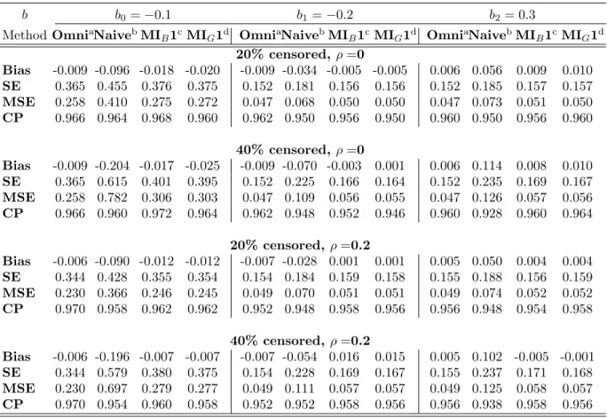
Table 1: Simulation Results of Multiple Imputation for One Marker at a Time

b b0=−0.1 b1=−0.2 b2= 0.3

MethodOmnia_Naiveb_MI

B1cMIG1d OmniaNaivebMIB1cMIG1d OmniaNaivebMIB1cMIG1d

20% censored,ρ=0 Bias -0.009 -0.096 -0.018 -0.020 -0.009 -0.034 -0.005 -0.005 0.006 0.056 0.009 0.010 SE 0.365 0.455 0.376 0.375 0.152 0.181 0.156 0.156 0.152 0.185 0.157 0.157 MSE 0.258 0.410 0.275 0.272 0.047 0.068 0.050 0.050 0.047 0.073 0.051 0.050 CP 0.966 0.964 0.968 0.960 0.962 0.950 0.956 0.950 0.960 0.950 0.956 0.960 40% censored,ρ=0 Bias -0.009 -0.204 -0.017 -0.025 -0.009 -0.070 -0.003 0.001 0.006 0.114 0.008 0.010 SE 0.365 0.615 0.401 0.395 0.152 0.225 0.166 0.164 0.152 0.235 0.169 0.167 MSE 0.258 0.782 0.306 0.303 0.047 0.109 0.056 0.055 0.047 0.126 0.057 0.056 CP 0.966 0.960 0.972 0.964 0.962 0.948 0.952 0.946 0.960 0.928 0.960 0.964 20% censored, ρ=0.2 Bias -0.006 -0.090 -0.012 -0.012 -0.007 -0.028 0.001 0.001 0.005 0.050 0.004 0.004 SE 0.344 0.428 0.355 0.354 0.154 0.184 0.159 0.158 0.155 0.188 0.156 0.159 MSE 0.230 0.366 0.246 0.245 0.049 0.070 0.051 0.051 0.049 0.074 0.052 0.052 CP 0.970 0.958 0.962 0.962 0.952 0.948 0.958 0.956 0.956 0.948 0.954 0.958 40% censored, ρ=0.2 Bias -0.006 -0.196 -0.007 -0.007 -0.007 -0.054 0.016 0.015 0.005 0.102 -0.005 -0.001 SE 0.344 0.579 0.380 0.375 0.154 0.228 0.169 0.167 0.155 0.237 0.171 0.168 MSE 0.230 0.697 0.279 0.277 0.049 0.111 0.057 0.057 0.049 0.125 0.058 0.057 CP 0.970 0.954 0.960 0.958 0.952 0.952 0.958 0.956 0.956 0.938 0.958 0.956

a_Omni_{: Omniscient,} b_Naive_{: Censored observations replaced by LOD/2,} c_MI

B1: MI-Bootstrapping, dMIG1: MI-Gibbs sampling

For the case when the two markers are independent or weakly correlated, we applied our Gibbs sampling based MI method for one marker at a time and compared the results to the bootstrap based MI approach presented by Lubin et al. [32]. In the bootstrap based procedure, a bootstrap sample was generated first from the observed data with replacement and the Tobit likelihood function was used to obtain the estimates ˜βand ˜σ2_{. Then the}

cen-sored observation was imputed by a value generated from the inverse cumulative distribution function

Φ−1{UNIF[0,Φ(d; ˜β,σ˜2)]; ˜β,σ˜2}, (3.9) where UNIF[0, a] is a uniform distribution on [0, a]. For each of these data sets we compared an omniscient estimate (Omni) obtained from the complete data, an naive estimate (Naive) based on replacing censored observation by LOD/2, a MI estimate based on bootstrapping

(34)

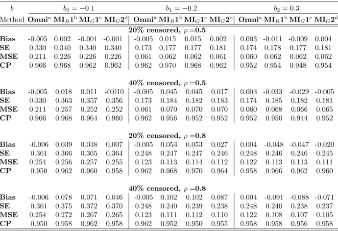
(MIB1) and the MI estimate based on Gibbs sampling (MIG1). Note that the correlation between markers was essentially ignored in MIB1 and MIG1 as they were applied for the censored markers one at a time. Table1summarizes the results obtained from the simulation study where each of the two markers is treated independently in the analysis. As expected, the two MI approaches (MIB1 and MIG1) performed much better than the Naive method, even when the data are not heavily censored (i.e., 20%). The naive substitution with LOD/2 yielded significantly biased estimates and larger SEs and MSEs. Compared to the Omni method, which serves as the gold standard, both of the MI approaches consistently produced approximately unbiased estimates. The SEs, MSEs and CPs were also comparable. For the setting where we incorporate the correlation between two markers, we conducted a simulation study similar to that outlined above. As shown in Table 2, the estimates from methods

MIB1 and MIG1 are considerably biased for the effects of censored markers, even though the intercept estimates remained fine when the censoring and correlations are not high (20% censoring, ρ = 0.5). In contrast, method MIG2, the MI method accounting for marker correlations, still resulted in unbiased estimates for all of the coefficients when censored markers are highly correlated. Even when the correlation is moderate (ρ = 0.5), method

(35)

Table 2: Simulation Results of Multiple Imputation for Higher Correlated Markers

b b0=−0.1 b1=−0.2 b2= 0.3

Method Omnia_MIB1b_MIG1c_MIG2d _Omnia_MIB₁b_MIG1c_MIG2d _Omnia_MIB1b_MIG1c_MIG2d

20% censored, ρ=0.5 Bias -0.005 0.002 -0.001 -0.001 -0.005 0.015 0.015 0.002 0.003 -0.011 -0.009 0.004 SE 0.330 0.340 0.340 0.340 0.173 0.177 0.177 0.181 0.174 0.178 0.177 0.181 MSE 0.211 0.226 0.226 0.226 0.061 0.062 0.062 0.061 0.060 0.062 0.062 0.062 CP 0.966 0.968 0.962 0.962 0.962 0.970 0.968 0.962 0.952 0.954 0.948 0.954 40% censored, ρ=0.5 Bias -0.005 0.018 0.011 -0.010 -0.005 0.045 0.045 0.017 0.003 -0.033 -0.029 -0.005 SE 0.330 0.363 0.357 0.356 0.173 0.184 0.182 0.183 0.174 0.185 0.182 0.181 MSE 0.211 0.257 0.252 0.252 0.061 0.070 0.070 0.070 0.060 0.068 0.066 0.065 CP 0.966 0.968 0.964 0.960 0.962 0.956 0.952 0.952 0.952 0.950 0.944 0.952 20% censored, ρ=0.8 Bias -0.006 0.039 0.038 0.007 -0.005 0.053 0.053 0.027 0.004 -0.048 -0.047 -0.020 SE 0.361 0.366 0.365 0.364 0.248 0.247 0.247 0.246 0.248 0.246 0.246 0.245 MSE 0.254 0.256 0.257 0.255 0.123 0.113 0.114 0.112 0.122 0.113 0.113 0.111 CP 0.950 0.962 0.960 0.958 0.962 0.968 0.970 0.964 0.958 0.966 0.962 0.960 40% censored, ρ=0.8 Bias -0.006 0.078 0.071 0.046 -0.005 0.102 0.102 0.087 0.004 -0.091 -0.088 -0.071 SE 0.361 0.375 0.372 0.370 0.248 0.240 0.239 0.238 0.248 0.240 0.238 0.237 MSE 0.254 0.272 0.267 0.265 0.123 0.111 0.112 0.110 0.122 0.108 0.107 0.105 CP 0.950 0.958 0.962 0.958 0.962 0.952 0.950 0.955 0.958 0.958 0.956 0.958

a_Omni_{: Omniscient,} b_MIB₁_{: MI-Bootstrapping,} c_MIG1_{: MI-Gibbs sampling for single censored marker,}

d_MIG2_{: MI-Gibbs sampling accounting for correlations between markers}

3.4 APPLICATION

The Genetic and Inflammatory Markers of Sepsis (GenIMS) study was designed to identify genetic markers and biomarkers related to the development of severe sepsis as a result of community acquired pneumonia (CAP). The study enrolled 2,320 subjects with CAP from emergency department at 28 US hospitals. In addition, several secondary outcomes such as organ failure, acute kidney injury (AKI) and death were also examined. To assess the rela-tionship between potential biomarkers and these outcomes, biomarkers in the inflammatory

(36)

and coagulation pathways were measured daily during the first seven days of hospitalization and weekly thereafter. For the example presented here, we focused on the prediction of AKI using day 1 levels of cytokines and fibrinolysis markers. The analysis cohort included 1836 patients who were confirmed CAP cases admitted to the hospital and with available biomarker data. The markers analyzed for this example include tumor necrosis factor (TNF) which was censored at a lower limit of 4, interleukin-6 (IL6) which was censored at either 2 or 5 depending on the assay used, interleukin-10 (IL10) which was censored at 5, plasminogen activator inhibitor (PAI-1) which was censored at 2 and D-dimer which was censored at the lower limit of 110. The censoring proportions for these markers were 34.97%, 27.34%, 9.42%, 8.28% and 1.74%, respectively. We assumed a log-normal distribution for the biomarker concentrations and analyzed the data using the natural log scale. To apply the multiple imputation procedures, the means of each of the biomarkers were estimated. The biomarker means were modeled in the log scale using linear regression models that included baseline characteristics (age, gender and baseline creatinine as marker of kidney function) and the outcome variable AKI.

To assess the magnitude of correlations among these five markers, we used the method of Lyles et al. [41] to estimate the correlation coefficients between the two censored markers. The estimated correlation matrix is given by

             

IL6 IL10 TNF PAI-1 D-dimer

1.00 0.47 0.40 0.17 0.25 1.00 0.34 0.21 0.05 1.00 0.18 0.30 1.00 −0.01 1.00               ,

indicating that the correlations among the markers are small to moderate. The correlations among cytokines (IL6, IL10 and TNF) are relatively stronger than those between the two fibrinolysis markers (PAI-1 and D-dimer), so we only incorporated the cytokine correlations in the Gibbs-sampling based MI method (MIG2) and compared the results to those obtained from naive method, and two simple MI methods, MIB1 and MIG1. Table 3 provides the

(37)

estimates, standard errors and p-values of each risk factor for the development of AKI. The results from the four methods were similar for the adjusted baseline variables and markers with small amounts of censored data which are PAI-1 and D-dimer. However, there were noticeable differences across the four methods for the coefficient estimates and significance of cytokine effects, when both of the correlations and levels of censoring were higher. In particular, the effect of TNF became significant when the correlations between markers were incorporated in the MI method. These results are consistent with the simulation study. In all cases the MI methods outperformed the naive method when the censoring proportion reaches 20%. With censoring proportions of 30% or higher, it becomes important to ac-count for the correlations in the MI, even if the correlation is moderate (e.g, 0.4 or 0.5). Table 3: Analysis Results for Prediction of AKI using Day 1 Cytokines and Fibrinolysis Markers

Method Naive (LOD/2)a _MIB₁b _MIG1c _MIG2d

Parameter Est. SE p Est. SE p Est. SE p Est. SE p Intercept -7.917 1.055 .000 -7.942 1.064 .000 -7.626 1.045 .000 -8.020 1.068 .000 Age 0.041 0.007 .000 0.041 0.007 .000 0.041 0.007 .000 0.040 0.007 .000 Male -0.625 0.254 .014 -0.617 0.254 .008 -0.630 0.255 .007 -0.634 0.251 .006 Creatinine 2.418 0.819 .003 2.375 0.821 .002 2.473 0.826 .001 2.435 0.810 .001 logIL6 0.070 0.052 .177 0.070 0.053 .094 0.061 0.052 .125 0.012 0.048 .407 logIL10 0.027 0.077 .723 0.032 0.074 .336 0.036 0.075 .319 0.065 0.076 .204 logTNF 0.157 0.096 .104 0.178 0.101 .047 0.124 0.085 .077 0.282 0.099 .003 logPAI-1 0.211 0.075 .005 0.220 0.077 .002 0.219 0.076 .003 0.221 0.087 .006 logD-dimer 0.241 0.090 .008 0.240 0.092 .004 0.202 0.083 .014 0.251 0.094 .004

Censoring proportion: IL6(9.42%),IL10(34.97%),TNF(27.34%), PAI-1(8.28%), D-dimer(1.74%)

a_Naive_{: Censored observations replaced by LOD/2,} b_MIB₁_{: MI-Bootstrapping,}

c_MIG1_{: MI-Gibbs sampling for single censored marker,}

d_MIG2_{: MI-Gibbs sampling accounting for correlations between cytokines (IL6, IL10 and TNF)}

3.5 DISCUSSION

Censoring issues due to lower or upper detection limits are not uncommon in biomarker studies, but it is often not well-documented at the data collection and can be easily neglected in the analysis stage. Motivated by the GenIMS study, we proposed MI procedures based on the Gibbs sampling method for multiple censored markers. Markov Chain Monte Carlo

(38)

(MCMC) methods such as the Gibbs sampler have been widely used for imputing data with non-monotone missing patterns. We extended these MI methods to left-censored biomarker data by incorporating the informative missing mechanism (which is known to be due to the detection limit) in the MI procedure. Although various modeling approaches were developed for analyzing censored marker data as response variables, the evaluation of diagnostic and prognostic performance of markers usually requires marker measurement to be treated as predictors/covariates. The MI approach provides a practical and flexible solution for further complex analysis. Our MI methods performed well for low to moderate levels of censoring in the data (20%∼40%) and can easily accommodate right-censored or interval-censored data. Our simulation results showed that ignoring the correlations between censored markers may lead to biased estimates in the logistic regression when the correlation is high or moderate and the data are heavily censored. Our method requires the assumption of a multivariate normal distribution, which may not be satisfied with marker data. Appropriate transformations (e.g., Box-Cox transformation) need to be considered. When the amount of missing data is not large, there is evidence [61] that inference made from the MCMC based imputed data tend to be robust to departures from the normal distribution. Whether this is the case for censored data and how the choices of prior distributions affect the results merit further study.

(39)

4.0 MEDIAN REGRESSION FOR LONGITUDINAL LEFT-CENSORED RESPONSES

Biomarkers are often measured repeatedly in biomedical studies to help understand the devel-opment of the disease, identify the patients at high-risk and guide the therapeutic strategies for intervention. One common source of measurement error for biomarkers is left-censoring because the assays used may not be sensitive enough to measure the low concentrations below a detection limit. The likelihood-based approaches assuming multivariate normal distribu-tion have been proposed to account for left-censoring problem; however the biomarker data are often highly skewed even after certain transformations. We propose a median regression model that requires minimal assumption on the distribution and leads to easier interpreta-tion of the results in the original scale of the data. We developed the estimating procedures incorporating correlations between serial measurements for left-censored longitudinal data. We conducted simulation studies to evaluate the properties of the proposed estimators and compare median regression model with mixed models under various specifications of distri-butions and covariance structures. We demonstrated our method with a data set from the Genetic and Inflammatory Markers of Sepsis (GenIMS) study.

4.1 INTRODUCTION

Biomarkers are often measured repeatedly in biomedical studies for gaining insight of ment effectiveness and establishing the potential disease pathways to guide the future treat-ment targets. However, the biomarker data are subject to various sources of measuretreat-ment errors. Left-censoring due to the lower limit of detection (LOD) is a common source of

(40)

error that may not be noticed in the analysis stage of biomarker data. In the Genetic and Inflammatory Markers of Sepsis (GenIMS) study (Kellum et al. [3]), a set of inflammatory and coagulation markers were evaluated repeatedly during the course of hospitalization for patients with community acquired pneumonia. Unfortunately, the assays used were not sen-sitive enough to measure low concentrations of some biomarkers, resulting in moderate to heavy left-censoring data. Figure 1 presents the censoring proportion of cytokines, TNF (tumor necrosis factor), IL6 (interleukin-6) and IL10, over the first week of hospitaliza-tion. Since left-censoring introduces informative missing data that are not ignorable, the traditional longitudinal analyses based on mixed model and generalized estimating equation (GEE) approach are no longer valid.

The ad-hoc methods using an arbitrary constant such as LOD, LOD/2, or LOD/√2 usually lead to biased estimation results. The existing statistical methods for left-censored data mainly focuses on the likelihood-based approach, where the distribution of censored variable is fully specified. The contribution of censored observations to the likelihood func-tion is indicated by the probability of being censored. For example, a normal distribufunc-tion is assumed in the Tobit linear regression model (Tobin [71]; Persson and Rootzen [49]) for inde-pendent data. Mixed models based on the idea of Tobit model have been developed for the left-censored longitudinal data with various computational algorithms presented by different researchers (Hughes [29]; Lyles et al. [42]; Jacqmin-Gadda et al. [31]; Wu [75]; Thiebaut et al. [70]). A Tobit variance-component method was demonstrated in linkage analysis of family left-censored trait data (Epstein et al. [15]). However, the normality assumption of mixed models may not be satisfied as the biomarker data are often highly skewed even after certain transformation. Additionally, misspecification of covariance structure of response variable in the mixed models may result in biased estimates. The GEE methods are usually considered as a robust alternative to mixed models, but incorporation of left-censoring data in GEE methods is not trivial without specifying the distribution of censored variable. In the literature of econometrics, quantile regression has been popularly used due to its robustness to non-normality or heteroscedasticity. The corresponding quantile regression methods for data censored at a fixed constant were also well established (Powell [50, 51]). However the computation of censored quantile regression estimators and associated variance estimators