Conditional Moment Tests for Parametric Duration Models
James E. Prieger∗ Department of Economics
University of California One Shields Avenue Davis, CA 95616-8578 [email protected]
November 7, 2000
Abstract
This paper develops and compares specification tests for parametric duration models esti-mated with censored data. The tests are based on generalized residuals (the integrated hazard), which is exponentially distributed if the model is correctly specified. I present several condi-tional moment tests based on the generalized residuals: a raw moments test, a test based on Laguerre polynomials, and a Lagrange multiplier (LM) test. The LM test extends Lancaster’s (1985) test by allowing an arbitrarily precise approximation of the likelihood under the alter-native. The raw moments test implemented via an auxiliary regression is examined using both asymptotic and bootstrap critical values. Monte Carlo evidence indicates that no one test dom-inates the others in all situations in terms of size, power, and ease of use. When the data are not censored, the Laguerre test appears to be the best choice. When there is censoring in the data, the Laguerre test is still at least as powerful as the other tests, but the raw moment test may be more convenient to perform. For the convenience of the practitioner the explicit forms of the tests for exponential and Weibull duration models are presented.
∗This paper is based on chapter 3 of my dissertation (Prieger, 1999). I thank seminar participants at UC Davis,
and especially Colin Cameron, for helpful comments. Earlier versions of the paper benefitted from comments from Alan Marco, Enrico Moretti, Roger Studley, and seminar participants at UC Berkeley. The inevitably remaining mistakes are inevitably mine. PRELIMINARY: PLEASE DO NOT CITE WITHOUT PERMISSION.
Keywords: right censoring, type I censoring, duration analysis, exponential distribution, Weibull distribution, specification test, power curve, bootstrap bias.
1
Introduction
In the linear regression model, correct specification of the distribution of the error term is not necessary for consistent maximum likelihood estimation of regression coefficients as long as the conditional mean is correctly specified as x0iβ. This robustness to distributional misspecification,
however, does not extend to most duration models, especially those involving censoring. Spec-ification testing is therefore important in censored duration models. The leading examples of misspecification in duration models are neglected heterogeneity and duration dependence. One response to the non-robustness of duration models to misspecification has been to develop semi-parametric regression methods. The commonly-used Cox (1972) proportional hazards model makes no assumptions about duration dependence, but assumes there is no heterogeneity not captured by observed covariates.1 An alternative response to the problem of misspecification is to use
para-metric models, but to subject them to specification tests.2 This paper develops and compares specification tests for parametric duration models estimated with right-censored data.
Many specification tests for duration models have sprung up (Lancaster, 1985; Horowitz and Neumann, 1989; Jaggia, 1991; Sharma, 1992; Jaggia, 1997). A natural building block for specifi ca-tion testing in duraca-tion models is the estimated integrated hazard, which can be viewed as a gener-alized residual. The integrated hazard is unit exponentially distributed if the likelihood is correctly specified, no matter what the duration distribution is. Departures from the assumed duration dis-tribution show up as departures of the generalized residual from the exponential disdis-tribution, which is the basis for graphical (Jaggia and Thosar, 1995) and statistical (Lancaster, 1985; Sharma, 1992)
1
See Horowitz (1999) and the citations therein for estimation methods for the proportional hazards model with unobserved heterogeneity.
2
Methods such as “semi-nonparametric” series expansion (Gallant and Nychka, 1987) blur the distinction be-tween parametric and semiparametric estimation and lend an arbitrary amount offlexibility to maximum likelihood estimation.
tests based on generalized residuals.3 There are few applications of such tests for censored data, however, a gap this paper attempts to fill.
Testing based on residuals often fits into the framework of the conditional moment test of Newey (1985) and Tauchen (1985). Conditional moment tests have been studied and performed mostly for complete (i.e., uncensored) observations. When some observations are censored in the data, as they often are, the tests must use censored moments (and their expectations) for those observations. Pagan and Vella (1989) provide such a way to incorporate censored observations into conditional moment tests in the context of tobit models.4 I present three conditional moment tests modified for censored duration data in the spirit of Pagan and Vella (1989): a raw moments test, a test based on Laguerre polynomials, and a Lagrange multiplier test. The contribution of the paper is to expand the arsenal of available tests for censored duration data, to examine thefinite-sample performance of the tests, and to discuss implementation issues for the practitioner.
The conditional moment test is appealing to practitioners for two reasons. First, one need estimate only the single model one wishes to test. Unlike Wald or likelihood ratio tests, one does not need to estimate a more general model that nests the model of interest. Even Lagrange multiplier (LM) tests must be constructed with reference to an alternative hypothesis that requires a more general model, and the derivation of the variance of the statistic can be quite involved. Conditional moment tests require only that one generate some form of residuals from the estimated model and combine them into various statistics for the test. Second, conditional moment tests are appealing because they can be quickly implemented via an auxiliary regression that obviates calculation of the variance matrix for the test statistic.5 I show that the auxiliary regression method leads to highly inaccurate inference in small samples, however, which the bootstrap does not remedy when the null hypothesis is false. In particular, although the bootstrap corrects the size problem of the
3Given that generalized residuals can be constructed for any parametric model, not just duration models, the tests presented here can be used for any parametric model. I concentrate on the application to duration models.
4In the same paper, Pagan and Vella (1989) discuss tests for duration data, but only for uncensored observations. 5
As appealing as the conditional moment test is, it is not an omnibus test. There will be some alternatives against which the test has no power (Newey, 1985).
auxiliary regression test, the power curve exhibits severe bias. I develop the Laguerre test as a more accurate and powerful alternative that is not difficult to implement.
The results of the paper indicates that the performance of the Laguerre test at least weakly dominates the others in terms offinite-sample accuracy and power. When the data are not censored, the Laguerre test is as powerful as the LM test that is optimal against the alternative considered, and the Laguerre test as easy or easier to implement as any of the tests. When there is censoring in the data, the Laguerre test is still at least as powerful as the other tests, but the raw moment test may be more convenient to perform. Adding higher moment conditions to the tests does not improve power against heterogeneity when the baseline hazard rate is correctly specified but does improve power against duration dependence in the baseline hazard.
I proceed in the next section by introducing the notation and framework for conditional moment testing of duration models, following Pagan and Vella (1989). In section 3, I present a test based on raw moments of the generalized residuals, which illustrates how the moment conditions are modified for censored data. Jaggia (1991) discusses similar moment-based tests, but only for uncensored data. In section 4, I develop a test based on Laguerre polynomials similar to that of Sharma (1992), but extended for censored data. The Laguerre polynomial test has the computationally convenient property that for some distributions it is asymptotically orthogonal.
Section 5 extends Lancaster’s (1985) LM test for unobserved heterogeneity. Jaggia (1997) extends Lancaster’s (1985) LM test to include censored data; I further extend it to allow an arbitrarily precise approximation of the likelihood under the alternative of heterogeneity. Higher-order approximation of the likelihood in the LM test turns out to be analogous to adding higher-order moments in moment-based tests. In section 5, I also discuss the kinship between the three tests. The Monte Carlo results in section 6 show that the Laguerre and LM tests generally fare well against the raw moment/auxiliary regression tests. For the convenience of the practitioner, an appendix provides the explicit forms of the tests for exponential and Weibull duration models.
2
The Conditional Moment Approach to Testing
2.1
The Moment Conditions
Let the hazard function of the duration random variable Y >0be
h(y, x,θ0)≡ lim
∆y→0
Pr (y≤Y < y+∆y|Y ≥y,θ0, x)
∆y , (1)
the probability of a spell of lengthy ending the next instant, conditional on lasting at least as long asy, on parameter vectorθ0, and on vector of`explanatory variablesx. The parameter vectorθ0,
with dim(θ0) =k < ∞, may comprise ` coefficientsβ0 and additional k−`nuisance parameters
(such as the Weibull shape parameter). Define
ε(y, x,θ0)≡
Z y
0
h(t, x,θ0)dt, (2)
the integrated hazard, to be thegeneralized error in the sense of Cox and Snell (1968).6 The PDF and CDF of the duration process can be stated in terms of the hazard function:
f(y|x,θ0) = h(y, x,θ0) exp (−ε(y, x,θ0)) (3)
F(y|x,θ0) = 1−exp (−ε(y, x,θ0)) (4)
(see, e.g., Lancaster, 1985). Ifhis continuous iny, thenhmay be replaced with ∂ε/∂y in (3) and
the PDF may be expressed entirely in terms ofε.
Consider an independent latent sample {y∗i} from Y, i= 1, . . . , N. Let the observed sample {yi} be censored, with fixed right censoring points {ci} and censoring indicators {di} such that yi = min{y∗i, ci} and di = 1{yi = ci}, where 1{·} is the indicator function.7 For the rest of
the paper, asterisks will denote latent, uncensored quantities, so that ε∗
i ≡ε(yi∗, xi,θ0) and εi ≡
ε(yi, xi,θ0). Then the contribution to the likelihood of a censored observation yi is Pr(Y > 6Note thatεdoes not have mean zero; for that reason some authors (Pagan and Vella, 1989) prefer to define the generalized error asε−E(ε). I do not follow this convention here. See Gourieroux, Monfort, Renault and Trognon (1987) for another definition of generalized errors.
7
yi|xi,θ0) =1−F(yi|xi,θ0), and the log likelihood of the observed sample is l(θ) = N X i=1 (1−di) logh(yi, xi,θ)−ε(yi, xi,θ). (5)
The conditional moment approach to specification testing exploits the fact that if the model is correctly specified, the sample average moments (evaluated at the estimated parameters and the ob-served explanatory variables) should be close to the population moment expectations. In a Gaussian model, for example, one might examine the residual vector ei ≡yi−E(yi) for heteroskedasticity
and non-normal kurtosis by looking at the quantities N−1Px i ¡ e2 i −σb2 ¢ and N−1P ¡e4 i −3σb4 ¢ , respectively.
Although one could develop tests for duration models based on residuals {ei}, it is convenient
to specify moment conditions in terms ofε∗, becauseε∗ is exponentially distributed forany hazard function (Crowley and Hu, 1977). Therefore moment conditions based on ε∗ will be the same no matter what the duration distribution is, implying that the conditional moment tests will have general applicability. I assume the moment conditions of interest can be written in terms ofε∗i or
εi. Let m∗: R++ →Rq be a vector of conditional moments. Denotem0i∗ ≡m∗(ε∗i) and construct m∗ so that
E¡m0i∗|xi
¢
=0, i=1, . . . , N. (6)
If the uncensored sample {y∗i}were observed, one could base a specification test on the sample analog of (6). Letˆθbe the maximum likelihood (ML) estimate of θ0, and defineˆε∗i ≡ε
³
yi∗, xi,ˆθ
´ , and mˆ∗i ≡m∗(ˆε∗i).8 Then the q dimensional vector
ˆ τ∗≡ 1 N N X i=1 ˆ m∗i (7)
will be close to zero in the latent sample if the moment restrictions are true in the population.
Censoring complicates matters slightly. Pagan and Vella (1989), in the context of the tobit model, suggest taking the expectation of (6) conditional on the censoring. Lettingwi = (xi, ci, di)
and m0
i ≡m0(εi, wi)≡E[m∗(ε∗i)|εi, wi], by the law of iterated expectations and (6) we have:
E©m0i|xi, ci
ª
= 0, i=1, . . . , N. (8)
In (8), expectation is taken over (εi, di). Thus specification tests for censored samples may be
based on the sample analog of (8). Lettingˆεi ≡ε
³
yi, xi,ˆθ
´
andmˆi≡m(ˆεi, wi), the statistic
ˆ τ ≡ 1 N N X i=1 ˆ mi (9)
will be close to zero in the censored sample if the moment restrictions are true in the population. The rest of this section presents two asymptotically equivalent test statistics based on (9). The trade-offbetween the two, as we will see, is one of convenience versus power.
2.2
The Test Statistic
To find the asymptotic distribution of ˆτ under the null hypothesis that the model is correctly
specified and that (6) holds, assume that the following probability limits exist:
M0 q×k≡ plimN−1X∇θ0m(ε(yi, xi,θ), wi)|θ=θ0 J0 k×k≡ − plim 1 N ∇θθ0l(θ)|θ=θ0 N−12 X · m0i0 gi00 ¸ d →N( 0 (q+k),(q+k)V×0(q+k) ) (10)
where the subscripts denote the dimensions of the matrices, summations run from 1 toN, andgi0 ≡ g(yi, wi,θ0) is the(k×1) derivative of theith contribution to the log likelihoodl: g0i =∇θli|θ=θ0.
It will be useful below to partition the variance matrix as:
V0 = Vmm0 Vmg0 Vgm0 Vgg0 (11)
Then it is straightforward to show (Pagan and Vella, 1989) that when ˆθ is the ML estimator we have √ Nˆτ →d N(0,Σ0), (12) where Σ0 =Vmm0+M0J0−1Vgm0+Vmg0J0−1M00 +M0J0−1Vgg0J0−1M00. (13)
By the information equality, for an independent sampleJ0 =Vgg0. Furthermore, by the generalized
information equality (Tauchen, 1985), E(∇θ0m0i) = −E(mi0gi00), and it follows that M0 =−Vmg0. These results combine to simplify the expression for the variance to two equivalent forms:
Σ0 = Vmm0 −Vmg0Vgg−10Vgm0 (14)
= Vmm0 −M0J0−1M00 (15)
A convenient form for the test is
Nτˆ0Σ−01τˆ→d χ2(q), (16)
which requires an estimate ofΣ0 to be feasible.
Under independent sampling, the terms on the right-hand side of (14) will be the following expectations: V0 ≡E µ E ½· m0i0 gi00 ¸0· m0i0 gi00 ¸¯¯¯¯xi ¾¶ . (17)
ThereforeV0 can be consistently estimated withVˆ, the usual sample average analog of (17)
evalu-ated at the estimevalu-ated parameter vectorˆθ. Define Σˆ to be the estimate ofΣ0 based onVˆ and (14).
The test statistic (16) using Σˆ may be written as
N2ˆτ0nS0hI−G¡G0G¢−1G0iSo−1ˆτ →d χ2(q), (18)
whereGis the N×kmatrix with ˆg0i=g(yi, wi,ˆθ) as theith row, and S is theN ×q matrix with 0
maker” for a linear regression. That is, the expression in braces is composed of the squared, summed residuals from regressing mˆi on gˆi. Tauchen (1985) shows that one can therefore implement the
test via an auxiliary regression: regressmˆi ongˆi and a constant (this will be a seemingly unrelated
regression [SUR] if q > 1) and test the constant(s) for significance. The resulting test statistic is
N2ˆτ0nS0hI−G(G0G)−1G0iS
−τˆτˆ0o−1τˆ, which differs from (18) only by the presence of τˆτˆ0 in the braced expression, which converges in probability to 0 under the null hypothesis. Thus testing via the auxiliary regression is asymptotically equivalent to testing based (16) usingΣ, and the twoˆ are nearly equivalent in finite samples. The auxiliary regression method is convenient, in that it can be implemented with any regression software.
While the auxiliary regression method is asymptotically equivalent to (16) and is easy to imple-ment, it has notorious slow convergence to its limiting distribution (Pagan and Vella, 1989). In the simulations performed in Section 6, Ifind that the actual small sample size of the raw moment test may be over six times its nominal level. As an alternative to the auxiliary regression, when Y fol-lows the exponential distribution one can easily calculate the inner expectation in (17) analytically, and then average over thexi in the sample to approximate the outer expectation. This analytical
estimate generally converges to its probability limit faster thanVˆ in practice, and performs better thanVˆ in Monte Carlo power studies (Jaggia, 1997). The analytical estimate is
ˇ V =N−1XE ½· m00 i gi00 ¸0· m00 i gi00 ¸¯¯¯ ¯xi ¾¯¯¯ ¯ θ=ˆθ (19)
and is used in the Monte Carlo exercise below for the Laguerre and LM tests. Define Σˇ to be the estimate ofΣ0 based onVˇ. AlthoughVˇmm0, the upper left partition of (19), can be calculated for any distribution for the moment tests considered in this paper,Vˇmg0 and Vˇgg0 may not be available for models other than the exponential.
Afinal possible estimate ofV0 can be based on the sample average analogs ofVmm0,M0, andJ0
in (15) when Vˇmg0 and Vˇgg0 are not available. This estimate, Σ, replaces the appropriate elements˜ of (15) with Vˆmm0 ≡ N−1Pmˆimˆ0i, Mˆ ≡ N−1
P
performance of the auxiliary regression method, testing based on (16) using Σ˜ may be preferred for models for whichΣˇ cannot be easily calculated (e.g., the Weibull model).
Section A.1 in the appendix contains the explicit form of Σˇ for the exponential model and of ˜
Σfor the Weibull model when the second through fourth moment conditions are used in the three versions of the test presented in the next three sections. Section A.1 also presents the gradient for these models needed to implement the auxiliary regression.
3
Tests Based on Raw Moments
Which moments should one use for testing? Given a fully specified distribution under the alternative hypothesis, an LM test defines the optimal set of conditional moments (Newey, 1985). In practice, one often chooses a test based not only on its asymptotic power but on its ease of implementation.9 The practitioner may choose among the infinite number of moments satisfying (6). In this section and the next two, I explore three alternative sets of moments based on the generalized residuals.
Most tests using generalized residuals in the literature are based on raw moments. Here I present the raw moment conditions for censored samples. Becauseε∗ is distributed unit exponential, theq
population raw moment conditions corresponding to (6) are:
m0i∗ q×1 = ε∗i2−2! .. . ε∗iq+1−(q+1)! . (20)
If there is no censoring in the sample, test statistics can be based directly on the sample analogs of the theoretical moments. Let the element ofτˆ∗ in (7) corresponding to thepth power ofˆε∗i be:
rp∗= 1 N N X i=1 ¡ ˆε∗ip−p!¢. (21) 9
It has been humorously noted that the actual power of a test is the theoretical power multiplied by the probability that the test is actually used.
In the censored sample, instead of (20) one calculates m0
i, the expectation of m0i∗ conditional on
the censoring. To do this, note that when the error is not censored, we have
E¡ε∗ip|εi, di = 0
¢
=εpi, (22)
and that when the error is censored, we have
E¡ε∗ip|εi, di=1 ¢ = p X j=0 p! j!ε j i; (23)
see section A.2.2 from the appendix.
From (22) and (23), we find the appropriate element of ˆτ in (9) (the counterpart to r∗p for censored samples) to be:
rp= 1 N N X i=1 ˆεpi −p! +di p−1 X j=0 p! j!ˆε j i (24)
Note thatrp reduces to the usual raw moment conditions for uncensored observations when di = 0
for alli. Typically one takesˆτ = (r2, . . . , rq+1)0; one cannot testr1 (refer to discussion of equation
(49) below). Of particular interest are thefirst few moments:
r2=N−1 X ˆε2i −2 + 2di(ˆεi+1) (25) r3=N−1 X ˆε3i −6 + 3di ¡ ˆ ε2i + 2ˆεi+ 2 ¢ (26) r4 =N−1 X ˆ ε4i −24 + 4di ¡ ˆ ε3i + 3ˆε2i + 6ˆεi+ 6 ¢ (27) where all summations are over 1 to N. Many practitioners use raw moments and the auxiliary regression form of the test to avoid the matrix calculation of the variance matrix.
4
Tests Based on Laguerre Polynomials
This section develops an alternative to raw moment tests, in which the moments are chosen to be orthonormal polynomials in the generalized residual. Such tests, under certain circumstances, are particularly easy to implement, requiring no matrix computation of Vˆ. Furthermore, the Monte
Carlo exercises in section 6 show that the Laguerre tests avoid the slow asymptotic convergence of the auxiliary regression method.
Letf(Z|x,θ)denote the conditional density of a random variableZ.Assume that the moments
ωp=E(Zp|x,θ)exist and arefinite for allp∈N. A family of polynomials{Pp(Z, x,θ)}∞p=0, where
pis the order of the polynomial, is said to be orthonormal with respect to density f if
E(Pn(Z, x,θ)Pp(Z, x,θ)|x,θ) =1{n=p}. (28)
When the even moments dominate the others, orthonormal polynomial families always exist and are unique.10 The orthonormal polynomial family for the (uncensored) exponential distribution is the family of Laguerre polynomials. Thepth Laguerre polynomial inZ is
Lp(Z) = p X j=0 (−1)j p! (j!)2(p−j)!Z j, (29)
where the usual convention 0! =1 holds.11 Because L0 is 1, it follows from (28) thatE(Lp) = 0.
Note that because the generalized error is exponentially distributed for any duration distribution, the Laguerre polynomials inε are orthonormal for any data generating process.
Sample moments for censored observations based on Laguerre polynomials take the form
λp = 1 N N X i=1 (1−di)Lp(ˆεi) +diL˜p(ˆεi) (30)
for the appropriate element ofτˆ in (9), whereLp is as in (29), and
˜ Lp(y) = p X j=0 (−1)j µ p j ¶Xj m=0 ym m!
is the expectation of the Laguerre polynomial when the duration is censored. Thefirst few moment
1 0
In particular, letΩbe the matrix with ij elementωi+j−2. Then ifΩ is positive definite, there exists a unique
orthonormal polynomial family with respect tof (Cramér, 1946). The converse also holds. 1 1
One can show by direct calculation that (29) satisfies the recurrence relation defining the Laguerre polynomials: (p+1)Lp+1(Z) = (2p+1−Z)Lp(Z)−pLp−1(Z)(Abramowitz and Stegun, 1964, p.782).
conditions from Laguerre polynomials are λ2 = N−1 X1 2 £ ˆ ε2i −4ˆεi+ 2 + 2di(ˆεi−1) ¤ (31) λ3 = N−1 X1 6 £ −ˆε3i + 9ˆεi2−18ˆεi+ 6 + 3di ¡ −ˆε2i + 4ˆεi−2 ¢¤ (32) λ4 = N−1 X 1 24 £ ˆ ε4i −16ˆε3i + 72ˆε2i −96ˆεi+ 24 + 4di ¡ ˆε3i −9ˆε2i +18ˆεi−6 ¢¤ (33)
When there is no censoring,di = 0for all iand λp reduces toλ∗p=N−1
P
Lp(ˆε∗i).
Sharma (1992), building on work by Kiefer (1985), showed (for uncensored data) that condi-tional moment tests based onλpmay be derived as an LM test for unexplained duration dependence.
In that case the nesting model is an expansion of (3) by means of Laguerre polynomials inεi, and
the restricted model with no unexplained duration dependence is (3).
Although the Laguerre polynomials (29) are orthonormal with respect to the uncensored ex-ponential distribution, the modified Laguerre polynomials (30) are not orthonormal–or even orthogonal–with respect to the censored exponential distribution. Although one can construct orthonormal polynomials for the censored exponential distribution by the Gram-Schmidt method, the coefficients of the resulting polynomials are tedious to compute. Given that the advantage of the orthonormal polynomials–their ease of computation (explained below)–is lost in the censored case, I do not present the orthonormal polynomials for the censored distribution.
In some cases orthonormal polynomials lead to test statistics that are particularly easy to compute. The test statisticτˆ is asymptotically orthogonal if the asymptotic variance matrix ofτˆ
is diagonal. Asymptotically orthogonal tests are desirable because the variance matrix is easy to compute, sequential tests are invariant to the order in which they are performed, and joint test statistics are the sum of individual test statistics. For an example of the latter, the test statistic for the joint test that (λ2,λ3,λ4) = 0 would be the sum of the test statistics for each individual
test ofλi= 0,i= 2,3,4.
Laguerre-based tests are orthogonal only under certain conditions. Tests using (30) are not or-thogonal when some data are censored, because then{λp}is not an orthogonal set of polynomials.
Even for uncensored data, orthonormal polynomials do not necessarily lead to orthogonal tests. Orthonormality of the moments ensures thatVmm0 is diagonal, but the second term in (15) may not be diagonal. The variance matrixΣ0 is diagonal, and hence the test is asymptotically orthogonal,
if M0 ≡ plimN−1
P
∇θ0m0i = 0. The Laguerre polynomial moments have this property for the exponential model, but they do not for many other commonly used duration models. Although Sharma (1992) conjectures that asymptotic orthogonality is unlikely to extend out of the exponen-tial case, the following proposition (proved in the appendix) shows that asymptotic orthogonality can be extended to some other distributions.
Proposition 1 For any uncensored duration random variableyi with generalized error of the form
εi = καiΛ(yi), with κi = exp(−β0xi), α 6= 0 a known constant, and Λ a known function, under
independent sampling we have M0 = plimN−1P∇θ0m0i = 0, where m0i are the Laguerre moment
conditions.
For such processes with no censoring, then, (14) implies that the asymptotic variance is merely
Vmm0. The orthonormality of the Laguerre polynomials furthermore means that Vmm0 = I; i.e. the Laguerre tests are asymptotically orthogonal. Thus calculating the joint test statistic in the uncensored case requires no variance computations or matrix inversions, and in the censored case onlyVmm0 need be calculated and inverted. The class of processes withεi =καiΛ(yi) is a subset of
the proportional hazards class; the baseline hazardΛ must be known and contain no elements ofθ.
The most important member of this class is the exponential duration model. For the exponential model,Λ(yi) =yi. The class also includes the Rayleigh distribution, commonly used in life testing
of electronic components. The class does not contain the lognormal or log-logistic models, and includes the Weibull model only if the shape parameter is known. Table 1 characterizes these models.
5
An LM Test for Unobserved Heterogeneity
A third set of moments may be derived from an LM test for unobserved heterogeneity. This section extends Lancaster’s (1985) LM test for neglected heterogeneity in the hazard rate in two directions. Lancaster’s (1985) test is for uncensored samples, and is a true LM test only up to a second order approximation of the likelihood. I first modify the test to include censored data, as did Jaggia (1997). I then use higher-order approximations of the likelihood function in the construction of the test statistic, which leads to a test with higher power.
Let the hazard function of the duration process, (1), take the formh(y|v, x,θ0) =vb(y, x,θ0),
v >0. Herevis a multiplicative heterogeneity term satisfyingE(v) =1, andbis a baseline hazard rate. A leading example of such a hazard function has b(y, x,θ0) = e−x0β0 and heterogeneity
parameterized as v = exp (−u), so that the hazard is h(y) = exp (−[x0β0+u]). This is the form used in the Monte Carlo exercises, but results here will be developed for the general form here.
Define εb to be the integrated hazard from (2) when v = 1. In terms of εb the conditional
survival functionS(y)–the fraction of durations lasting longer than y–is
S(y|v, x,θ0)≡1−F(y|v, x,θ0) = exp(−vεb), (34)
where the dependence ofεbon(y, x,θ0)is suppressed in the notation. Equation (34) follows directly
from (4). The unconditional (on v) survival function is
S(y|x,θ0)≡1−F(y|x,θ0) =Ev[exp(−vεb)]. (35)
Finally, let E(v−1)p = µ
p , the pth central moment. Recall µ1 = 0; fixing the mean allows
5.1
Approximating the Unrestricted Likelihood
To explore heterogeneity in the duration model, approximate (34) withS˜q+1, an expansion of order q+1(q≥1) ofS as a function of v aboutv=1: ˜ Sq+1(y|v, x,θ0) = S(y|v=1, x,θ0) + q+1 X p=1 dp dvpS(y|v, x,θ0) ¯ ¯ ¯ ¯ v=1 (v−1)p p! (36) = e−εb 1+ q+1 X p=1 ap(εb) (v−1)p , (37)
where (37) follows from (34) and ap(ε) ≡ (−ε)p/p!. Taking expectations with respect to v, we find: ˜ Sq+1(y|x,θ0) =S(y|v=1, x,θ0) 1+ q+1 X p=2 ap(εb)µp . (38)
Given that the PDF f equals−S0, it follows that f may be approximated by−S˜q0+1:
˜ fq+1(y|x,θ0) =f(y|v=1, x,θ0) 1+ q+1 X p=2 [ap(εb) +ap−1(εb)]µp (39)
Equation (39) follows from (38) and the fact that ε0b(y) ≡ b(y).Therefore f is approximated by (39) whenµ2 and the higher moments (i.e., the heterogeneity) are small.
Now the approximate likelihood of a sample including censored and uncensored observations follows directly. As before, let the indicator variable di be 1 if duration yi is censored and 0
otherwise. Then (5), (38), and (39) lead to l¡θ, µ2, . . . , µq+1¢, an approximation of the true log likelihood of the sample:
l¡θ, µ2, . . . , µq+1¢ = N X i=1 (1−di) logbi−εbi+ log 1+ q+1 X p=2 [ap(εbi) +ap−1(εbi)]µp +di log 1+ q+1 X p=2 ap(εbi)µp −εbi , (40) wherebi ≡b(yi, xi,θ) and εbi≡εb(yi, xi,θ).
5.2
The LM Test Statistic
Recall the idea of the LM test is that the score (expected first derivatives of the log likelihood function) of the unrestricted model will be close to zero when evaluated at the restricted estimates, if indeed the restrictions are true. A general form of the test is
h ∇θ0logLU(ˆθR) i h IU(ˆθR) i−1h ∇θlogLU(ˆθR) i d −→χ2(q), (41)
whereLU is the likelihood of the unrestricted model, IU is the information matrix from the
unre-stricted likelihood,ˆθR is the vector of estimates from the restricted model, andq is the number of
restrictions. In the present context, our parameter vector of interest is¡θ, µ2, . . . , µq+1¢≡(θ, µ). The restriction we wish to test is µ= 0.
The average gradient of (40) may be found from
N−1∇θl(θ, µ) = N−1 N X i=1 (1−di) µ ∇θbi bi − ∇θ εbi ¶ +di(−∇θεbi) + q+1 X p=2 o¡µp¢ (42) N−1∇µpl(θ, µ) = N−1 N X i=1 (1−di)∇µplog 1+ q+1 X j=2 [aj(εbi) +aj−1(εbi)]µj (43) +di∇µplog 1+ q+1 X j=2 aj(εbi)µj (44)
for p = 2, . . . , q+1. Because the restricted estimation will be the same as the ML performed in section 2, we can denote ˆθR by ˆθ without ambiguity. Now, notice that because ˆθ maximizes the
restricted likelihood, (42) will be zero when evaluated at(ˆθ,0). Thus, in the statistic (41), all the
elements of the outer vectors are zero except for the derivative with respect to µ. The gradient with respect toµ, evaluated at the restricted parameter estimates, are
sp ³ ˆ θ, x´=∇µpl³ˆθ,0´= N X i=1 [ap(ˆεi)−(1−di)ap−1(ˆεi)]. (45)
Of particular interest are thefirst fewsp: s2 = N−1 X1 2 £ ˆε2i −2ˆεi+ 2diˆεi ¤ (46) s3 = N−1 X −1 6 £ ˆ ε3i −3ˆε2i + 3diˆε2i ¤ (47) s4 = N−1 X 1 24 £ ˆ ε4i −4ˆε3i + 4diˆε3i ¤ . (48)
Rather than calculating the variance matrix from (41) directly, we instead note that sp is a
conditional moment and that the test may be implemented by the methods in sections??and ??.
5.3
The Kinship Between the Tests
The moment conditions from the raw moments (rp), Laguerre polynomials (λp), and LM test for
heterogeneity (sp) are closely related. Since the LM test uses the theoretically optimal weighting
of the moments against the alternative hypothesis of multiplicative heterogeneity,12 other
moment-based tests can be viewed as sub-optimal weightings of the moments. When the coefficients β0 enter the hazard through exp(−x0
iβ0) (the usual parameterization)
and xcontains a constant, then λp and sp are linear combinations of(r1, . . . , rp) for all p, where
r1 =N−1
X ˆ
εi−1+di. (49)
Under these conditions, equationr1 is numerically set to zero when evaluated at the ML estimate;
it is the first-order condition for the constant from the maximization of the likelihood. In these cases the relationships among the moment conditions are
λp = p X j=1 ξpjrj (50) sp = 1 p!(−1) p(r p−prp−1) (51)
where ξpj is the coefficient on Zj in Lp(Z); see (29). For p = 2, all three conditional moments
are numerically equal when evaluated at the ML estimate of θ. For the uncensored case, the
1 2
An LM test is an asymptotically locally most powerful invariant test of the null hypothesis vs. the alternative against which it is constructed. Furthermore, infinite samples the LM test is alocally most powerful invariant test
equivalence betweens2 andλ2 was noted by Sharma (1992) and the equivalence betweenr2 and s2
was noted by Pagan and Vella (1989).13 The result here extends this equivalence to the censored case and shows that the higher moment conditions (p > 2) are not equivalent. Therefore, in general the performance of the tests will differ in finite samples when moments higher then the second are included.
An interesting equivalence between the LM and Laguerre tests holds forp even larger than two when the distribution of the data are exponential and Σˇ based on (19) is used to form the test statistics. In that case the LM and Laguerre test statistics are numerically equivalent, even though the moment conditions differ. This equivalence holds whether the data are censored or not, but it is unknown if it would extend to distributions other than the exponential.14 The equivalence does
not hold ifΣ0 is estimated withΣˆ orΣ.˜
Recall that the Laguerre tests may be derived as an LM test for unexplained duration depen-dence. The equivalence of the Laguerre moments to the LM moments for unobserved hetero-geneity whenp= 2follows from the kinship between duration dependence and heterogeneity. For example, it is well known that neglected heterogeneity induces apparent duration dependence into the sample and that duration dependence causes over- or under-dispersion (see, e.g., Barlow and Proschan, 1965). The kinship between duration dependence and heterogeneity is also a warn-ing against attachwarn-ing a structural interpretation to one or the other in any particular application; structural duration dependence will appear in the data as heterogeneity, and vice versa.
6
Monte Carlo Results
In this section I examine the small sample performance of four versions of the above tests applied to an exponential regression model: 1) the raw moments test performed via the auxiliary regression
1 3
Prieger (1999) shows that a test based on centered moments matches the LM test even for higher moments. 1 4When the second and third moments are used and there is no censoring, the difference between the test statistics can be shown to be proportional to r1, and therefore zero when evaluated at the ML estimate. For other cases, I
method with asymptotic critical values, 2) the raw moments test performed via the auxiliary regression method with bootstrap critical values, 3) the Laguerre polynomial test using Σˇ [based on (19)], and 4) the LM test usingΣ. It is worth emphasizing the the auxiliary regression methodˇ could be used with any conditional moment test, including the Laguerre and LM tests, and that aΣˇ version could also be calculated for the raw moment test. I choose these four test versions for the following reasons. Version 1 appears to be the most commonly advocated test. For example, it is the specification test and method presented for duration data in Greene (2000), a standard graduate-level econometrics text. Given the known performance problems of version 1 and the increasing popularity of the bootstrap in econometrics, version 2 is a plausible next step after version 1. Version 3 is convenient to calculate in many cases, as explained in section 4. Version 4 is the optimal test for the alternative hypotheses in the Monte Carlo design, and so is the benchmark for the other tests.
The Monte Carlo exercises had the following design:
• The duration model is exponential, with PDF given by (52) in the appendix. The explicit moment conditions, gradient, and variance estimates are in section A.1 of the appendix.
• x is composed of a constant and a standard normal random variable. The regressors and
β00= (1,2)are fixed throughout all simulations.
• Heterogeneity takes the formv =e−u, wherev is as in (34) and u ∼N
³ σ2
2 ,σ2
´
, implying thatv has a lognormal distribution with E(v) =1.15 This is a special case of multiplicative
heterogeneity, the alternative hypothesis against which the LM test is optimal.
• The data are right-censored, withfixed censoring pointcchosen to achieve a desired percent-age of censoring in the data.
Considerfirst the performance of the tests when only the second moments are used. As is
known in the literature (e.g., Chesher and Spady, 1991), test statistics from auxiliary regressions converge very slowly to their asymptotic distribution. The asymptotics rely on the outer product of the gradient of the log likelihood to estimate the variance, which is known to have bad small-sample properties. The problem is exacerbated because the statistics rely on small-sample averages of high powers ofε, which can be poor estimates of the true expectations. Table 2 presents the actual
size of the tests based on second moments, for various sample sizes and levels of censoring. The
first column shows that the size of the raw moments test is far from the nominal 5% level when the asymptotic critical value is used, unless the sample sizes are large. The actual test size is about 11% when the sample size is 250 and about 7.5% when the sample size is 1,000. Censoring does not appear to make the distortion worse. When sample sizes increase to 10,000, the size drops to near the correct level, although the bias is still significant for the no-censoring case. Thus although the auxiliary regression method is convenient, it may lead to incorrect inference unless sample sizes are large. The use of the bootstrap (column two) clears up the size distortion quite well for all levels of censoring and sample sizes. None of the bootstrap sizes shows significant bias.
(Table 2 about here)
The sizes of the Laguerre and LM tests are in the final column of Table 2 (recall that the test statistics are identical for the exponential null hypothesis). The sizes of the Laguerre and LM tests tend to be on the low side, more so for smaller sample sizes, although the distortion is small compared with the auxiliary regression method. At the cost of additional computation, the bootstrap could be used to improve the sizes of these tests.
When the second and third moments are used together, the size distortion of the auxiliary regression method is greater than when the second moment alone is used (see Table 3). The levels with the second and third moments are about three times the levels with only the second moment when the sample size is 1,000 or smaller. The test statistic including the third moment contains higher powers of ε than the second-moment-only version, and the standard error of the sample
moments ofεrises with the order. The additional randomness apparently adversely affects the size
of the test. Once again, the bootstrap (second column) removes most of the size distortion of the auxiliary regression tests. The sizes of the Laguerre and LM tests are again on the low side for smaller sample sizes.
(Table 3 about here)
The power of the tests against the alternative of multiplicative heterogeneity as in (34) is depicted infigures 1, 2 and 3 for various levels of censoring (none, 25%, and 50% of the sample). In these figures the second and third moment conditions are used and the sample size is 250.16 When there is no additional variance from heterogeneity (i.e. σ2 = 0), the null hypothesis is true,
and the plotted point is the size of the test. The amount of heterogeneity increases along the horizontal axis, which is scaled in the graphs to be the percentage increase in the variance of the latent duration variable due to the heterogeneity.
(figure 1 about here) (figure 2 about here) (figure 3 about here)
The power curves reveal the following points. First, the size distortion of the auxiliary regression raw moments test with asymptotic critical values contrasts markedly with the relatively accurate bootstrap, LM, and Laguerre tests. Second, as one would expect, the power of the tests decreases as the amount of censoring in the sample increases. As the censoring becomes more severe, there is less information in the sample.17 Third, both auxiliary regression tests (raw moments with asymptotic and bootstrap critical values) are biased: for small amounts of heterogeneity there is a smaller
1 6
The bootstrap sample size is 99 and 100,000 iterations are performed. The power is evaluated at 8 to 16 points and curves are smoothed for plotting.
1 7
chance of rejecting the null hypothesis when false than when true.18 The bias persists over a large range of alternatives in the bootstrapped test.19 The bootstrap test is consistent20 because the auxiliary regression with the true critical value is consistent in this case (Horowitz, 1997, sec. 4.6), so the bias is purely a small sample phenomenon. These results are unfortunate, however, given the convenience of auxiliary regression tests. Fourth, the Laguerre and LM tests have identical power curves (figure 1). The exponential durations, along with use of (19) to estimate the variance, ensures that the LM and Laguerre tests are numerically indistinguishable, as explained in the previous section. In such cases the Laguerre test should be used because it is easier to calculate. Finally, to the right of the region of bias the asymptotic version of the raw moments test has lower power than the Laguerre and LM tests.
Figure 4 shows the power curves with a larger sample size of 1,000 observations. The power of all the tests is higher, and the range of bias of the bootstrap test is smaller. By the time the sample size increases to 10,000 observations (Figure 5), the range and magnitude of the bootstrap bias is quite small, although the test is still less powerful than the Laguerre and LM tests.
(figure 4 about here) (figure 5 about here)
A final question concerns the number of moments to use in the tests. Theoretically, the more moments used the higher the power of the test. This is most easily seen for the LM test: the more moments, the more accurate is the approximation of the likelihood in (39). Practically, however, the advantage of using higher moments is mitigated by the difficulties stemming from included higher powers of ε. As noted above, higher powers of ε take ever longer to converge to
their theoretical averages, and may degrade the performance of the test. The trade-off appears
1 8
This odd finding of bootstrap bias has been found in at least one other setting. In one of the bootstrapped information matrix tests for the tobit model Horowitz (1994) examines, the power against the examined alternative is less than the size.
1 9
The power curve of the bootstrapped test does eventually approaches 100% (offthe scale of the graph infigures1— 3).
2 0
to go against adding higher moments for the alternative hypotheses of correct baseline model specification but neglected heterogeneity, as in the Monte Carlo design above. Figure 6 shows the power of the LM and Laguerre tests (for N=250 and 25% censoring) as higher moments are added. The power of the test generally falls a bit when the third moment is added to the test compared to the second moment only, and falls further when the fourth moment is added to the test. Adding higher moments is likely to be of most use when the baseline duration model is incorrectly specified (Jaggia, 1991). To explore this, I run the LM and Laguerre tests when the true data generating process is lognormal and there is no heterogeneity. The lognormal distribution exhibits duration dependence, while the exponential distribution does not, so this example considers power against omitted duration dependence. The results are in Table 4. Adding higher moments did increase the power of the test: a 40% rejection rate with the second moment, a 49% rejection rate with second and third moments, and a 63% rejection rate with second, third, and fourth moments.
(Figure 6 about here) (Table 4 about here)
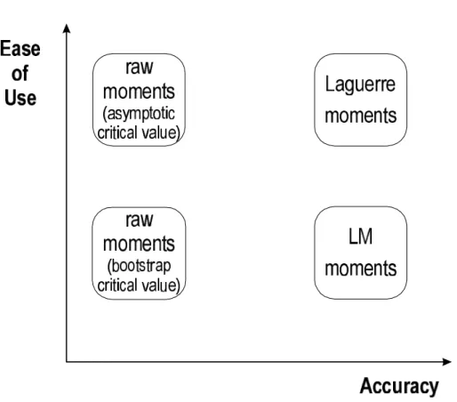
The comparison among the tests is summarized informally in figures 7 and 8. In these graphs, the “ease of use” of the tests is plotted against their “accuracy”. “Ease of use” refers generally to the amount of effort required to perform the test. The auxiliary regression test without bootstrapping places the fewest demands on the econometrician and on computer time, and thus is easiest to use. When there is no censoring, the Laguerre test is about as easy to implement because no variance or matrix calculations are required. The other tests are “less easy” because they require more computer time (e.g. bootstrapping) or more effort manipulating matrices. The “accuracy” of the test is an informal amalgamation of size and power. The auxiliary regression tests score low in this dimension due to bad size (the asymptotic version) or bias in the power curve (the bootstrap version). When the data are not censored,figure 7 shows that the Laguerre test is highest in both dimensions, making it the logical choice. When there is censoring, the bootstrap test is dominated
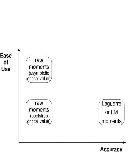
but which of the other tests is chosen depends on the taste of the econometrician.21 Note that all these comparisons are based on the exponential simulations, to which proposition 1 applies. If the duration distribution does not satisfy the conditions of proposition 1, then the comparison among the tests would look likefigure 8 for both censored and uncensored data.
(figure 7 about here) (figure 8 about here)
7
Conclusion
The raw moment specification test performed via auxiliary regression is probably the most com-monly used specification test for duration data. Despite the size problems with the test, Pagan and Vella (1989, p.S34) “suspect that the fact that the procedure is so easy to compute will make it attractive to many investigators....” As the bootstrap becomes more commonly used, it is natural to expect its application for these tests to clear up the size distortion. The simulations in this paper show that although the bootstrap does correct the size of the auxiliary regression test, it does so at the cost of bias and low power in general, so that this procedure cannot be recommended. I propose the Laguerre test as an alternative that is just as easy to perform as an auxiliary regres-sion when the data are not censored and the model is exponential (or another model satisfying the conditions of proposition 1). Furthermore, the Laguerre test has higher power than either form of the raw moment test for most alternatives studied, and the same power as the optimal LM test. Adding higher moment conditions to the tests does not improve power vs. heterogeneity when the baseline hazard rate is correctly specified but does improve power when the baseline hazard itself is misspecified due to omitted duration dependence. The Laguerre and LM tests are useful new tools to assess the specification of models for censored duration data.
2 1
References
Abramowitz, Milton and Stegun, Irene (1964),Handbook of Mathematical Functions, with
Formu-las, Graphs, and Mathematical Tables, Vol. 55 ofUnited States, National Bureau of Standards,
Applied Mathematics Series, Washington, D.C.
Barlow, Richard E. and Proschan, Frank (1965), Mathematical Theory of Reliability, New York: John Wiley & Sons.
Chesher, Andrew and Spady, Richard (1991), ‘Asymptotic Expansions of the Information Matrix Test Statistic’, Econometrica 59(3), 787—815.
Cox, David R. (1972), ‘Regression Models and Life-Tables’,Journal of the Royal Statistical Society,
Series B 34, 187—202.
Cox, David R. and Snell, E.J. (1968), ‘A General Definition of Residuals’, Journal of the Royal
Statistical Society B 30(2), 248—275.
Cramér, Harald (1946),Mathematical Methods of Statistics, number 9in ‘Princeton Mathematical Series’, Princeton University Press, Princeton.
Crowley, J. and Hu, M. (1977), ‘Covariance Analysis of Heart Transplant Survival Data’, Journal
of the American Statistical Association 72(357), 27—36.
Engle, Robert F. (1984), Wald, Likelihood Ratio, and Lagrange Multiplier Tests in Econometrics,
inZ. Griliches and M. Intriligator, eds, ‘Handbook of Econometrics. Volume II’, Handbooks in Economics, book 2, Amsterdam; New York: North-Holland Pub. Co., chapter 13, pp. 775—826.
Gallant, A. Ronald and Nychka, Douglas W. (1987), ‘Semi-Nonparametric Maximum Likelihood Estimation’,Econometrica 55(2), 363—390.
Gourieroux, Christian, Monfort, Alain, Renault, Eric and Trognon, Alain (1987), ‘Generalised Residuals’, Journal of Econometrics34, 5—32.
Greene, William H. (2000),Econometric Analysis, Upper Saddle River, N.J.: Prentice Hall. Horowitz, Joel L. (1994), ‘Bootstrap-Based Critical Values for the Information Matrix Test’,
Jour-nal of Econometrics 61, 395—411.
Horowitz, Joel L. (1997), Bootstrap Methods in Econometrics,inD. Kreps and K. Wallis, eds, ‘Ad-vances in Economics and Econometrics: Theory and Applications: Seventh World Congress. Volume 3.’, Econometric Society (Monographs, no.28), Cambridge: Cambridge U. Press. Horowitz, Joel L. (1999), ‘Semiparametric Estimation of a Proportional Hazard Model with
Unob-served Heterogeneity’, Econometrica67(5), 1001—1028.
Horowitz, Joel L. and Neumann, George R. (1989), ‘Specification Testing in Censored Regres-sion Models: Parametric and Semiparametric Methods’, Journal of Applied Econometrics
4(0), S61—S86, Supplement.
Jaggia, Sanjiv (1991), ‘Tests of Moment Restrictions in Parametric Duration Models’, Economics
Letters 37(1), 35—38.
Jaggia, Sanjiv (1997), ‘Alternative Forms of the Score Test for Heterogeneity in a Censored Expo-nential Model’,The Review of Economics and Statistics 79(2), 340—343.
Jaggia, Sanjiv and Thosar, Satish (1995), ‘Contested Tender Offers: An Estimate of the Hazard Function’, Journal of Business and Economic Statistics13(1), 113—119.
Kiefer, Nicholas M. (1985), ‘Specification Diagnostics Based on Laguerre Alteratives for Econo-metric Models of Duration’,Journal of Econometrics28(1), 135—154.
Lancaster, Tony (1985), ‘Generalised Residuals and Heterogeneous Duration Models: With Appli-cations to the Weibull Model’, Journal of Econometrics28(1), 155—169.
Newey, Whitney (1985), ‘Maximum Likelihood Specification Testing and Conditional Moment Tests’, Econometrica53(5), 1047—1070.
Pagan, Adrian and Vella, Frank (1989), ‘Diagnostic Tests for Models Based on Individual Data: A Survey’, Journal of Applied Econometrics4(0), S29—S59.
Prieger, James E. (1999), Regulation, Innovation, and the Introduction of New Telecommunications Services, PhD thesis, University of California, Berkeley.
Sharma, Sunil (1992), ‘On Specification Diagnostics for Econometric Models of Durations’,Journal
of Quantitative Economics 8(2), 285—307.
Tauchen, George E. (1985), ‘Diagnostic Testing and Evaluation of Maximum Likelihood Models’,
Journal of Econometrics30(1).
Tsiatis, Anastasios A. (1981), ‘A Large Sample Study of Cox’s Regression Model’, The Annals of
Statistics 9(1), 93—108.
A
Appendix
A.1
Application to the Exponential and Weibull Models
This section presents the specific form of the three tests for the exponential and Weibull duration models for the convenience of the practitioner. The tests work for any distribution; see section 2 for the general form of the test for other applications.
A.1.1 Exponential Model
For the exponential duration model with meanκ−i 1 = exp (x0iβ0), the PDF is
f(yi|xi,β0) =κiexp (−κiyi) = exp ³ −x0iβ0−yie−x 0 iβ0 ´ . (52)
There are no nuisance parameters (k=`). The moment conditions for the various tests are found by substituting
ˆ
εi =yiexp(−x0iβˆ) (53)
in (25)—(27), (31)—(33), and in (46)—(48).
Raw moments test The raw moments test from section 3 is typically implemented via the
auxiliary regression method (see section 2.2). The `-vector of scores for the auxiliary regression are
ˆ
gi= [ˆεi−(1−di)]xi (54)
for the ith observation for the exponential case. The moment conditions (25)—(27) are regressed via SUR on the scores and a constant and the constants are tested for significance.
Laguerre moments test For the Laguerre test from section 4, whenY is exponential and there
is no censoring, proposition 1 applies and the asymptotic varianceΣ0 of the test statistic (12) isI.
When there is censoring,Σ0 may be estimated byΣˇ based on (14) and (19). The elements ofVˇmm0 as defined in (19) resulting from the second through fourth moment conditions, (31)—(33), are:
ˇ v11 = 1−N−1X ¡ˆε2ci+1 ¢ exp (−ˆεci) (55) ˇ v12 = N−1 X µ1 2ˆε 3 ci −ˆε 2 ci+ ˆεci ¶ exp (−ˆεci) (56) ˇ v22 = 1−N−1 X µ1 4ˆε 4 ci−ˆε 3 ci+ 2ˆε 2 ci+1 ¶ exp (−ˆεci) (57) ˇ v31 = N−1 X µ −1 6ˆε 4 ci+ ˆε 3 ci− 3 2ˆε 2 ci+ ˆεci ¶ exp (−ˆεci) (58) ˇ v32 = N−1 X µ1 12ˆε 5 ci− 2 3ˆε 4 ci+ 2ˆε 3 ci−2ˆε 2 ci+ ˆεci ¶ exp (−ˆεci) (59) ˇ v33 = 1−N−1 X µ 1 36ˆε 6 ci− 1 3ˆε 5 ci+ 19 12ˆε 4 ci−3ˆε 3 ci + 3ˆε 2 ci+1 ¶ exp (−ˆεci) (60)
whereˇvijrefers to the(i, j)element of the submatrixVˇmm0,ˆεci =ε(ci, xi,ˆθ),ciis the right censoring
point, and all summations run from1 toN. The other elements of (14) for the censored case are
ˇ Vmg0 = −N−1Pˆε ciexp(−ˆεci)x0i N−1P12¡εˆ2ci−2ˆεci ¢ exp(−ˆεci)x0i −N−1P16¡ˆεc3i−6ˆε2ci+ 6ˆεci ¢ exp(−ˆεci)x0i (61) ˇ Vgg0 =N−1 X [1−exp(−ˆεci)]xix 0 i (62)
Note that when there is no censoring, ci (and therefore εci) may be taken to be infinite, so that
(55)—(60) simplifies to I and (61) is zero as claimed.
LM test for heterogeneity For the LM test from section 5, Σ0 may be estimated by Σˇ based
on (14) and (19). The elements ofΣˇ for the test statistic based on (46)—(48) are the following:
ˇ v11 = N−1 X h 2−¡ˆε2ci+ 2ˆεci+ 2 ¢ e−ˆεci i (63) ˇ v21 = −N−1 X µ 3−1 2 ¡ ˆε3c i+ 3ˆε 2 ci+ 6ˆεci+ 6 ¢ e−ˆεci ¶ (64) ˇ v31 = N−1 X µ 4− 1 6 ¡ ˆε4ci+ 4ˆε3ci+12ˆε2ci+ 24ˆεci+ 24 ¢ e−ˆεci ¶ (65) ˇ v22 = N−1 X µ 6− 1 4 ¡ ˆε4ci+ 4ˆε3ci+12ˆε2ci+ 24ˆεci+ 24 ¢ e−ˆεci ¶ (66) ˇ v32 = −N−1 X µ 10− 1 12 ¡ ˆ ε5ci+ 5ˆε4ci+ 20ˆε3ci+ 60ˆε2ci+120ˆεci+120 ¢ e−ˆεci ¶ (67) ˇ v33 = N−1 X µ 20− 1 36 ¡ ˆ ε6c i+ 6ˆε 5 ci+ 30ˆε 4 ci+120ˆε 3 ci+ 360ˆε 2 ci + 720ˆεci+ 720 ¢ e−ˆεci ¶ (68) ˇ Vmg0 =N−1 X 1−(ˆεci+1)e− ˆ εci −1+¡12ˆε2ci+ ˆεci+1 ¢ e−ˆεci 1−¡16ˆε3ci +21ˆε2ci+ ˆεci+1 ¢ e−ˆεci x0i (69) ˇ Vgg0 is as in (62).
A.1.2 Weibull Model
For the Weibull duration model (Weibull I from table 1), we have θ0 =
¡
β00,σ0
¢0; σ
0 is a scalar
shape parameter controlling duration dependence (dim(θ0) = `+1). The PDF and generalized
residual are f(yi|xi,θ0) = (σ0yi)−1 ³ yie−x 0 iβ0 ´1/σ0 exp · −³yie−x 0 iβ0 ´1/σ0¸ (70) and ˆ εi = h yiexp(−x0iβˆ) i1/σˆ . (71)
Raw moments test The(`+1)-vector of scores for the auxiliary regression (section 2.2) are
ˆ gi= 1 ˆ σ [ˆεi−(1−di)]xi ˆ εilog ˆεi−(1−di) (1+ log ˆεi) (72)
for theith observation for the Weibull case.22 The moment conditions (25)—(27) are regressed via
SUR on the scores and a constant and the constants are tested for significance.
Laguerre moments test Since the Weibull model with unknown shape parameter is not in the
class of distributions for which M0 = 0for the Laguerre tests (section 4), the asymptotic variance
of the Laguerre test does not simplify to I even when there is no censoring. For uncensored observations, Σˇ may be calculated as for the exponential model above. Vˇmm0 = I when there is no censoring (this is true for any distribution). The other elements needed forΣˇ for the Weibull model and moments (31)—(33) are:
ˇ Vgg0 = 1 ˆ σ2N X xix 0 i (1−γ)xi (1−γ)x0i 61π2+ (1−γ)2 = 1 ˆ σ2N X xix 0 i 0.422 78xi 0.422 78x0i 1.823 68 (73) ˇ Vgβm0 =0 (74) ˇ Vgσm0 = ˆσ− 1 · 1 1/2 1/3 ¸ (75)
2 2If a parameterization of σ such as ς = log(σ)is chosen for the ML routine, the final row of (72) needs to be adjusted accordingly.
whereγ= 0.577 21566is Euler’s constant.
Estimates (73)—(75) do not apply when the data are censored. The analytical estimate Σˇ in this case contains partial gamma, digamma, and trigamma functions, making it computationally unattractive. Therefore a simpler estimate of Σ0 is obtained from Σ, the estimate of˜ Σ0 based on
pluggingVˆmm0, Mˆ, and Jˆ into (15) (see section 2.2). Vˆmm0 ≡N−1Pmim0i is found by using the
summands of (31)—(33) formi. The other pieces ofΣ˜ are:
ˆ Mβ0 = 1 ˆ σN X εi −εi+ 2−di 1 2ε2i −3εi+ 3 +di(εi−2) −16ε 3 i + 2ε2i −6εi+ 4−di ¡1 2ε 2 i −3εi+ 3 ¢ x0i (76) ˆ Mσ = 1 ˆ σN X εilog(εi) −εi+ 2−di 1 2ε 2 i −3εi+ 3 +di(εi−2) −16ε3i + 2εi2−6εi+ 4−di ¡1 2ε2i −3εi+ 3 ¢ (77) ˆ Jββ0 = ¡ ˆ σ2N¢−1Xεixix0i (78) ˆ Jσβ0 =¡σˆ2N¢− 1X [(logεi+1)εi−(1−di)]x0i (79) ˆ Jσσ = ¡ ˆ
σ2N¢−1X[(logεi+ 2)εilogεi−(1−d) (2 logεi+1)] (80)
where Mˆβ0 contains the first ` columns (those pertaining to β0) of Mˆ,Mˆσ is the final column of ˆ
M, andJˆββ0,Jˆσβ0, and Jˆσσ are the obvious partitions of Jˆ.
LM test for heterogeneity For the LM test (section 5) with uncensored observations, Σˇ may
be calculated as for the exponential model above. Vˇmm0 = I, Vˇgg0 is as in (73), and the other elements needed forΣˇ for the Weibull model and moments (46)—(48) are:
ˇ Vgβm0 = (ˆσN) −1X xi · 1 −1 1 ¸ (81)
ˇ Vgσm0 = ˆσ− 1 2−γ γ− 52 17 6 −γ 0 = ˆσ−1 1.422 8 −1.922 8 2.2561 0 (82)
When the data are censored,Σ˜ should be used instead. Vˆmm0 ≡N−1Pmim0i is found by using
the summands of (46)—(48) formi. Jˆis as in (78)—(80). The other pieces ofΣ˜ are:
ˆ Mβ = 1 ˆ σN X εi −εi+ (1−di) 1 2ε 2 i −(1−di)εi −16ε 3 i +12(1−di)ε 2 i x0i (83) ˆ Mσ = 1 ˆ σN X εilog(εi) −εi+ (1−di) 1 2ε 2 i −(1−di)εi −16ε 3 i +12(1−di)ε 2 i (84)
where the definitions are as above.
A.2
Miscellaneous Results
A.2.1 Proof of Proposition 1
Consider ∇βλp, the pth element of m. We have ∇βλp = N1 PL0p(εi)∇βεi = −N1αPεiL0p(εi)xi,
so it suffices to show that E¡εiL0p(εi)
¢
= 0. For Laguerre polynomials, the recursion εiL0p(εi) =
p[Lp(εi)−Lp−1(εi)](Abramowitz and Stegun, 1964, p.783) and orthogonality property (28) imply
thatE¡εiL0p(εi)
¢
is indeed zero for allp.
A.2.2 Expectations of the censored generalized residual
The expectation ε∗
i when the observed variableεi is censored is:
E(ε∗i|εi, d=1) = Z ∞ ci ε(t, xi,θ0) f(t|xi,θ0) 1−F(ci|xi,θ0) dt
Using the identityε=−log(1−F) and change of variablesu=S(t) yields
E(ε∗i|εi, d=1) = [1−F(ci)]−1
Z 0
1−F(ci)
(−logu)(−du) =εi+1.
Similar calculation for higher powersε∗
i of leads to (23).
A.3
Monte Carlo Exercise Details
A particular simulation includes these steps:1. Load the initially generated and fixedx matrix, and form λ=e−x0β, anN ×1vector. This vector is heldfixed through all iterations.
2. Monte Carlo loop, to be performedRtimes for each particularσ2:
(a) Generate heterogeneity termv, an N ×1 vector, ifσ2 >0.
(b) GenerateN exponential random deviates of rate vλ.
(c) Censor the duration variable, if greater than the right-censoring pointc.23
(d) Compute the ML estimateβˆ forβ0.
(e) Form the generalized residuals and the moment conditions (and the score vector for the auxiliary regression tests).
(f) Form the test statistics using the desired moments:
i. Raw moments test statistic using (25) alone or both (25) and (26), generated via the auxiliary regression method described in sections 2.2 and A.1.1: regress the moment conditions on the scores and constants (a SUR if both (25) and (26) are used); form the joint test statistic for the significance of the constants. This statistic is referred to the asymptotic critical value for aχ2(1)orχ2(2)random variable as appropriate.
2 3
The censoring point is determined by a subroutine that performs steps (a) and (b) and picks the quantile of the resulting pseudo-data that leads to the desired level of censoring. These pseudo-data are then discarded. After
ii. Same as previous, but the statistic is referred to a bootstrap critical value. The size of the bootstrap sample is 999 for the size calculations and 99 for the power curves.24
iii. Laguerre polynomial test statistic using (31) alone or both (31) and (32) and the asymptotic variance as calculated in section A.1.1. This statistic is referred to the asymptotic critical value.
iv. LM test statistic using (46) alone or both (46) and (47) and the asymptotic variance as calculated in section A.1.1. This statistic is referred to the asymptotic critical value.
(g) Test the statistics using the relevant critical value, and record acceptance or rejection.
3. Report the percentage of rejections as the power of the tests for the chosen σ2.
2 4The method is the parametric bootstrap (Horowitz, 1997); the paired (natural) bootstrap yielded qualitatively similar results (including the persistance of the bootstrap bias).
Integrated Hazard
ε=£exp(−β0x)¤αΛ(y) Asymptotically Model Λ(y) α Orthogonal
exponential y 1 Yes
Rayleigh y1/2 0.5 Yes
proportional hazards Λ0(yi) 1 Yes∗
Weibull 1† y1/σ 1/σ No‡
Weibull 2† y1/σ 1 No‡
∗The baseline hazardΛ0 is taken to be known. If not, its estimation adds to the variance of the estimated generalized residual (Tsiatis, 1981) and the results of this paper do not apply.
†There are two forms of the Weibull model in the literature. ‡If the Weibull shape parameterσ is known, thenYes.
Table 1: Integrated Hazard and Asymptotic Orthogonality of the Laguerre Test for Various Distributions
Raw Moment Test Laguerre Asymptotic Bootstrap and LM Test Critical Values Critical Values Tests N = 250 No censoring 0.116∗ 0.050 0.041∗ 25% censoring 0.107∗ 0.050 0.041∗ 50% censoring 0.110∗ 0.050 0.040∗ N =1,000 No censoring 0.075∗ 0.050 0.048 25% censoring 0.073∗ 0.050 0.048∗ 50% censoring 0.074∗ 0.048 0.046∗ N =10,000 No censoring 0.056∗ 0.048 0.051 25% censoring 0.055 0.050 0.050 50% censoring 0.052 0.047 0.051
Table notes: Nominal size is 5%; * indicates significant (1% level) bias in the empirical size. N is sample size. Raw moment tests are performed via the auxiliary regression method (see section 2.2). Censoring is accomplished with a fixed right censoring point common to all observations. Bootstrap sample size = 999. For raw moment tests, number of Monte Carlo trials is 100,000 for N=250, 25,000 for N=1,000, and 10,000 for N=10,000. For Laguerre and LM tests, number of Monte Carlo trials is 100,000 for all sample sizes. The Laguerre and LM tests are numerically indistinguishable; the final column is the results from either test.
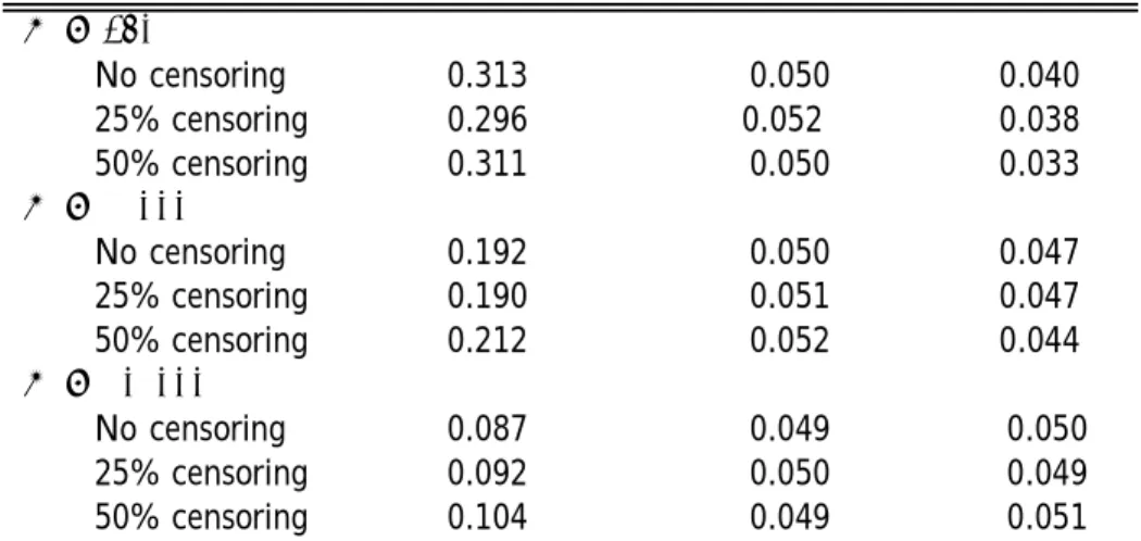
Raw Moment Test Laguerre Asymptotic Bootstrap and LM Test Critical Values Critical Values Tests N = 250 No censoring 0.313∗ 0.050 0.040∗ 25% censoring 0.296∗ 0.052∗ 0.038∗ 50% censoring 0.311∗ 0.050 0.033∗ N =1,000 No censoring 0.192∗ 0.050 0.047∗ 25% censoring 0.190∗ 0.051 0.047∗ 50% censoring 0.212∗ 0.052 0.044∗ N =10,000 No censoring 0.087∗ 0.049 0.050 25% censoring 0.092∗ 0.050 0.049 50% censoring 0.104∗ 0.049 0.051
Table notes: Nominal size is 5%; * indicates significant (1% level) bias in the empirical size. N is sample size. Raw moment tests are performed via the auxiliary regression method (see section 2.2). Censoring is accomplished with a fixed right censoring point common to all observations. Bootstrap sample size = 999. For raw moment tests, number of Monte Carlo trials is 100,000 for N=250, 25,000 for N=1,000, and 10,000 for N=10,000. For Laguerre and LM tests, number of Monte Carlo trials is 100,000 for all sample sizes. The Laguerre and LM tests are numerically indistinguishable; the final column is the results from either test.
Table 3: Empirical Levels of the Tests with Second and Third Moments Laguerre LM
Moments Test Test
Second 0.3951 0.3953
Second and Third 0.4901 0.4899 Second, Third, and Fourth 0.6357 0.6353
Table notes: N = 250. The true data generating process is lognormal with no heterogeneity; the (false) null hypothesis is an exponential model. Censoring is accomplished with a fixed right censoring point common to all observations so that 25% of the sample is censored. Number of Monte Carlo trials is 100,000.
Table 4: Power of the Laguerre and LM Tests vs. Incorrect Baseline Model as the Number of Moments Increases
Figure 1: Power curves for the tests vs. lognormal multiplicative heterogeneity (no censoring, 2nd and 3rd moments, N=250)
Figure 2: Power curves for the tests vs. lognormal multiplicative heterogeneity (25% censoring, 2nd and 3rd moments, N=250)
Figure 3: Power curves for the tests vs. lognormal multiplicative heterogeneity (50% censoring, 2nd and 3rd moments, N=250)
Figure 4: Power curves for the tests vs. lognormal multiplicative heterogeneity (25% censoring, 2nd and 3rd moments, N=1,000)
Figure 5: Power curves for the tests vs. lognormal multiplicative heterogeneity (no censoring, 2nd and 3rd moments, N=10,000)