Archive University of Zurich Main Library Strickhofstrasse 39 CH-8057 Zurich www.zora.uzh.ch Year: 2018
Kernelized Synaptic Weight Matrices
Muller, Lorenz K ; Martel, Julien N P ; Indiveri, GiacomoAbstract: In this paper we introduce a novel neural network architecture, in which weight matrices are re-parametrized in terms of low-dimensional vectors, interacting through kernel functions. A layer of our network can be interpreted as introducing a (potentially infinitely wide) linear layer between input and output. We describe the theory underpinning this model and validate it with concrete examples, exploring how it can be used to impose structure on neural networks in diverse applications ranging from data visualization to recommender systems. We achieve state-of-the-art performance in a collaborative filtering task (MovieLens).
Posted at the Zurich Open Repository and Archive, University of Zurich ZORA URL: https://doi.org/10.5167/uzh-168601
Conference or Workshop Item Published Version
Originally published at:
Muller, Lorenz K; Martel, Julien N P; Indiveri, Giacomo (2018). Kernelized Synaptic Weight Matrices. In: International Conference on Machine Learning 2018, Stockholm, 10 July 2018 - 15 July 2018, 3651-3660.
Lorenz K. Muller1 Julien N.P. Martel1 Giacomo Indiveri1
Abstract
In this paper we introduce a novel neural net-work architecture, in which weight matrices are reparametrized in terms of low-dimensional vec-tors, interacting through kernel functions. A layer of our network can be interpreted as introduc-ing a (potentially infinitely wide) linear layer be-tween input and output. We describe the theory underpinning this model and validate it with con-crete examples, exploring how it can be used to impose structure on neural networks in diverse applications ranging from data visualization to recommender systems. We achieve state-of-the-art performance in a collaborative filtering task (MovieLens).
1. Introduction
Neural Networks have a large number of free parameters and often training algorithms need to choose between a range of near optimal value assignments for those parame-ters. This choice can be difficult, because optimality with respect to a training set does not guarantee good behavior on unseen, similar data (especially when there are many free parameters). This defines overfitting. To address this problem, regularization techniques are widely used in Neu-ral Network optimization to help training procedures find generalizable solutions.
In this paper, we show that by expressing the weights of a neural network layer as the kernel interaction of low-dimensional vectors of free parameters, we can embed the weight matrix of a layer in some (potentially high-dimensional) feature-space; the embedding is controlled by the choice of the kernel function. This technique pro-vides a structural way to regularize weight matrices.
1Institute of Neuroinformatics, University of Zurich and ETH
Zurich, Switzerland. Correspondence to: Lorenz K. Muller <[email protected]>.
Proceedings of the35𝑡ℎ
International Conference on Machine Learning, Stockholm, Sweden, PMLR 80, 2018. Copyright 2018 by the author(s).
1.1. Related Work
There exist many approaches that reparametrize the weight matrix of a neural network. (Schmidhuber, 1997) and (Gomez & Schmidhuber,2005) learned weights for a neural network by training either small programs or another neural network respectively to generate them. The approach of training a neural network to generate weights for another network can take many forms and reoccurs for example in the work of (Stanley et al.,2009;Ha et al.,2016;Fernando et al.,2016). In (Koutnik et al.,2010) the weight matrix of a neural network is decomposed by a discrete cosine trans-form (DCT) and learning is pertrans-formed directly on the DCT parameters. Several recent papers propose different types of reparameterizations using various forms of matrix product decomposition (Denil et al.,2013;Moczulski et al.,2015; Tai et al.,2015).
Many methods have been proposed to ensure that at end of the training of a neural network the weights fulfill some desired properties: Weight-decay (or 𝐿2 regularization) (Krogh & Hertz,1992) makes large entries in the weight ma-trix costly, encouraging ‘simple’ models; drop-out ( Srivas-tava et al.,2014) (the inclusion of multiplicative Bernoulli noise) performs model averaging for appropriate network architectures, prevents co-adaptation of different weights, and can be interpreted as letting networks approximate deep Gaussian processes (Gal & Ghahramani,2016); low-rank de-composition of weight matrices (Sainath et al.,2013) (anal-ogous to separable convolutions in ConvNets (Jaderberg et al.,2014)) is primarily used for computational speed-up and memory footprint reduction, but also has a regularizing effect. As we shall see in this work, low-rank decomposition is a special case of the method we propose in this paper. In contrast to these approaches, our method allows the im-position of low-dimensional structure onto the network. We will show on several examples that the low dimensional embedding of the network weights does not only reduce the number of free parameters in a network, but has the advan-tage of increasing its interpretability as well as allowing for structural regularization.
1.2. Core Idea
Instead of assigning an individual, free weight-parameter between each input and output neuron of a neural network
layer, we associate with each input and each output a vector of free parameters that we think of as a location in a low-dimensional space. The weight between two units is then set to be some fixed function of the distance between those lo-cations (or more precisely a weighted kernel-function of the location vectors). A possible choice of kernel would be that neurons that are far away from each other are unconnected, neurons that are close to each other are strongly connected. Thus, the function of a layer is to produce a smooth kernel function, centered at the input locations, which is sampled at a few points by the output neurons (namely at their loca-tions).
2. Theory
2.1. Definition: kernelNet
We define a𝑑-dimensional kernelized neural network (𝑑-kernelNet) as a hierarchical function approximator on inputs ⃗
𝑥(0)and outputs𝑥⃗(𝑁)of the form:
𝑥(𝑗𝑙)=𝑓𝑗 ( ∑ 𝑖 𝛼𝑖(𝑙)𝐾(⃗𝑢(𝑖𝑙), ⃗𝑣(𝑗𝑙))𝑥(𝑖𝑙−1) ) . (1)
where super-scripts are layer indices, the functions𝑓𝑗 are
non-linearities, 𝛼𝑖 are scalar parameters, and 𝐾(⋅,⋅) is a kernel function that corresponds to an inner product, in some embedding space; i.e.
𝐾(⃗𝑢, ⃗𝑣) =⟨𝜙(⃗𝑢), 𝜙(𝑣⃗)⟩=⟨⃗𝑢∗, ⃗𝑣∗⟩ (2) with the embedding function𝜙∶ℝ𝑑→ℝ𝑑
∗
. The𝑑 dimen-sional vectors⃗𝑢,𝑣⃗are the free parameters of the model and ⃗𝑢∗, ⃗𝑣∗denote their embedded counterparts⃗𝑢∗ = 𝜙(⃗𝑢)and ⃗
𝑣∗=𝜙(𝑣⃗)of dimension𝑑∗.
Note that this is essentially a neural network layer, where the weight matrix𝐖has been replaced with a sum of weighted
kernels.
2.2. Relation to Fully-Connected Neural Networks In the special case of setting𝜙to the identity (and by con-sequence𝐾(⋅,⋅)to the dot-product) and setting𝛼𝑖= 1, we
obtain a fully-connected neural network, into each of whose layers a linear layer of a size𝑑has been interposed. Con-sider the activation of such a layer, before the non-linearity (as we consider a single layer, we left out the superscript of 𝛼,𝑢and𝑣for readability):
𝑥(𝑗𝑙) = ∑ 𝑖 𝛼𝑖𝐾(⃗𝑢𝑖, ⃗𝑣𝑗)𝑥(𝑖𝑙−1)=∑ 𝑖 𝛼𝑖⃗𝑢𝑇𝑖 𝑣⃗𝑗𝑥(𝑖𝑙−1) (3) = ∑ 𝑖 𝛼𝑖∑ 𝑘 𝑢𝑘𝑖𝑣𝑗𝑘𝑥(𝑖𝑙−1)=∑ 𝑘 𝑣𝑗𝑘∑ 𝑖 𝛼𝑖𝑢𝑘𝑖𝑥(𝑖𝑙−1)
Equation (3) describes a fully connected neural network layer with an intermediate layer, whose neurons with linear
...
...
(a)...
...
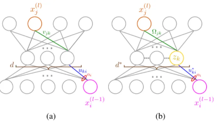
... ... (b)Figure 1.Illustrations to visualize the “virtual” layer introduced in
(a)Equation (3) and(b)Equation (4)
activation function are indexed by𝑘, as illustrated in Fig-ure1(a). We have connection matrices𝑢𝑘𝑖, 𝑣𝑗𝑘to and from
the linear layer. Alternatively we could interpret this as a product decomposition of the full weight matrix between 𝑥(𝑙)and 𝑥(𝑙−1). The dimension𝑑 in this case is the rank of the ‘effective’ weight matrix from𝑥(𝑖𝑙−1)to𝑥(𝑗𝑙). Such product decompositions are a well-known approach to neu-ral network regularization and compression (Sainath et al., 2013).
For choices of𝜙other than the identity, we obtain a virtual linear layer of dimension𝑑∗(that is potentially much greater than𝑑), and whose connection matrices are constrained by 𝜙. We compute the activation𝑥⃗(𝑙) before the activation function of the layer:
𝑥(𝑗𝑙)=∑ 𝑖 𝛼𝑖𝐾(⃗𝑢𝑖, ⃗𝑣𝑗)𝑥(𝑖𝑙−1)=∑ 𝑖 𝛼𝑖⟨𝜙(⃗𝑢𝑖), 𝜙(𝑣⃗𝑗)⟩𝑥(𝑖𝑙−1) =∑ 𝑖 𝛼𝑖⃗𝑢∗𝑖𝑇𝐌𝜙𝑣⃗∗𝑗𝑥 (𝑙−1) 𝑖 = ∑ 𝑖 𝛼𝑖 [ ∑ ℎ,𝑘 𝑢∗𝑘𝑖𝑀𝑘ℎ𝑣∗𝑗ℎ ] 𝑥(𝑖𝑙−1) =∑ ℎ,𝑘 𝑣∗ 𝑗ℎ𝑀𝑘ℎ [ ∑ 𝑖 𝛼𝑖𝑢∗ 𝑘𝑖𝑥 (𝑙−1) 𝑖 ] ⏟⏞⏞⏞⏞⏞⏞⏞⏞⏞⏟⏞⏞⏞⏞⏞⏞⏞⏞⏞⏟ 𝑧𝑘 =∑ 𝑘 𝑧𝑘 [ ∑ ℎ 𝑣∗ 𝑗ℎ𝑀𝑘ℎ ] =∑ 𝑘 𝑧𝑘Ω𝑗𝑘 (4)
where we used Eq.2and the Hermitian form of the inner product (note that𝐌𝜙 is necessarily symmetric positive
definite and is induced by𝜙).
In Equation (4) we can see that the proposed substitution corresponds to the insertion of a linear layer with unit acti-vations𝑧. The connections⃗ tothis layer are𝑢∗
𝑘𝑖andfromthis
layerΩ𝑗𝑘as illustrated in Figure1(b). These matrices are dependent on the free parameters as well as𝜙, which deter-mines their structure: Notably the index𝑘runs over the di-mensions of theembeddedvectors⃗𝑢∗, ⃗𝑣∗;𝜙prescribes how the finite entries of𝑣, ⃗𝑢⃗ make up these potentially infinite
(a) ⃗𝑢1⃗𝑢2 ⃗𝑢3 ⃗ 𝑣1 ⃗ 𝑣2 dim. 1 dim.2 Acti v ation (b)
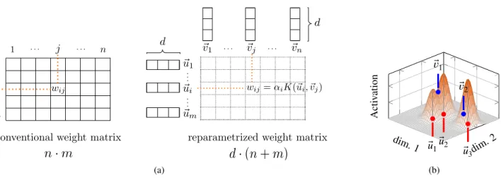
Figure 2.(a)Schematic comparison of a Kernelized and a standard synaptic weight matrix(b)Visualization of the activation of a layer with a two dimensional RBF Kernel of a3 × 2weight matrix. At the locations⃗𝑢𝑖we input a kernel (here a Gaussian) scaled by the input to
unit𝑖and𝛼𝑖. At the locations𝑣⃗𝑖we read out the height of the kernel sum.
dimensional vectors. The dimensionality of this embedding depends on the choice of𝜙or in practice𝐾(⋅,⋅). However, we never need to explicitly evaluate𝜙nor perform the dot product in𝑑∗.
The idea of using a kernel-function to get high-dimensional interactions between low dimensional vectors without need-ing to compute in the high-dimensional space, is known as the ‘Kernel-Trick’ in the kernelized machines literature, e.g. kernelized SVMs (Scholkopf & Smola,2001). In such kernelized SVM classifiers, instead of computing the dot-product between data points𝑥⃗and centroids 𝑐⃗𝑖 (that are
more usually called support vectors) of standard SVMs one evaluates a kernel function𝐾(𝑥, ⃗⃗ 𝑐𝑖). However this kernel takes data (⃗𝑥) as one of its arguments (the other one being a centroid, which in the case of SVM is also a data-point), while in our case both arguments are parameters.
In analogy to the standard fully-connected neural network layer, we can regard the kernelNet-layer as a fully-connected layer, whose weight matrix has been reparameterized by the parameters⃗𝑢, ⃗𝑣that are “decompressed" by a kernel func-tion𝐾(⋅,⋅). Notably the number of parameters of such a reparametrized weight matrix is only(𝑑⋅(𝑚+𝑛))rather than(𝑚⋅𝑛)(with𝑚the dimension of the input layer and 𝑛 the dimension of the output layer) as seen in Figure2. Hence, with our reparametrization, the number of parame-ters is reduced, as long as𝑑is less than half of the harmonic mean of𝑚and𝑛:𝑑 < 𝑚⋅𝑛
𝑚+𝑛 =
1
2(𝑚, 𝑛).
If the kernel function used in a kernelNet layer is differen-tiable, it can be trained through stochastic-gradient descent algorithms and its variants (see experiments in Section3).
2.3. Radial Basis Function Kernels
Some kernel functions can be visualized easily (at least for a low dimensional𝑑) and we will see that consequently also the input to neurons in a layer that uses this kernel can be visualized. A notable example of this is the Radial-Basis-Function (RBF) kernel, which has the form:
𝐾(⃗𝑢, ⃗𝑣) =𝛼⋅𝜓
(
𝐷(⃗𝑢, ⃗𝑣)) (5) where𝜓is a function𝜓 ∶ℝ+→ℝand𝐷(⋅,⋅)is a distance and𝛼∈ ℝ. Then we can interpret the𝑑-KernelNet layer as follows: Input channels place a kernel scaled by their activation (and by a basis weight𝛼) in a𝑑dimensional space centered at𝑢⃗𝑖, output neurons read the sums of these kernels at𝑣⃗𝑗. For an illustration see Figure2.
2.3.1. GAUSSIANRBF KERNELS The Gaussian RBF kernel
𝐾(𝑣, ⃗𝑢⃗ ) = exp(−𝛾||⃗𝑢−𝑣⃗||22) (6) is of theoretical interest because its embedding function𝜙 is well-known and maps into an infinite dimensional space (Scholkopf & Smola,2001). Furthermore outputs of this kernel can be interpreted as a similarity measure (it maps to 1 for identical vectors and asymptotically approaches 0 for very distant vectors).
2.3.2. FINITESUPPORTRBF KERNELS
RBF kernels whose support is finite can be used to impose a variable degree of sparsity (in a “𝐿0" sense) on the effective connectivity of the embedded network layer; this can be ap-plied to a non-kernelized network by expressing an effective weight matrix as the Hadamard-product of a unconstrained matrix and a finite-support kernel matrix.
Consider an embedding as above with𝑣⃗𝑗 fixed on a grid with grid constant𝑏. We can then use a finite support kernel
𝐾fs(⃗𝑢𝑖, ⃗𝑣𝑗) = max(0,1 −𝑎⋅𝐷(⃗𝑢𝑖, ⃗𝑣𝑗) )
(7) where𝐷(⋅,⋅)is a distance. By scaling𝑎and𝑏we can choose the maximal number of input neurons any given output neuron can get input from. Alternatively𝑣⃗𝑗 can remain free and a cost term of e.g. the form
𝑅=𝜆0
∑ 𝑖𝑗
(𝐾(⃗𝑢𝑖, ⃗𝑣𝑗))2, (8)
can be introduced, measuring the overlaps between “bumps", in which𝜆0will control the degree of sparsity of the trained model (see experiments in Section3.5).
A model of the form of Equation (7) must, by construc-tion, find a decomposition into independent sub-parts: Each input channel can only affect the activity of a few output channels. As the model becomes deeper, however, these sparse channels get mixed, so that for random connectivity the probability of an output to connect to a given 1st layer input, increases exponentially with the depth of the model.
3. Experiments
In the following experiments we demonstrate on some ex-amples, how kernelNets can be used in practice. We in-vestigate the effect of using different kernel functions (Sec-tion3.1), show how to incorporate prior knowledge into the network parameters (Section3.2), create extensible data visualizations (Section3.3,3.4) and achieve state-of-the art performance on the MovieLens dataset (Section3.5), while reducing the computational complexity of the model. 3.1. Impact of Effective Dimensionality
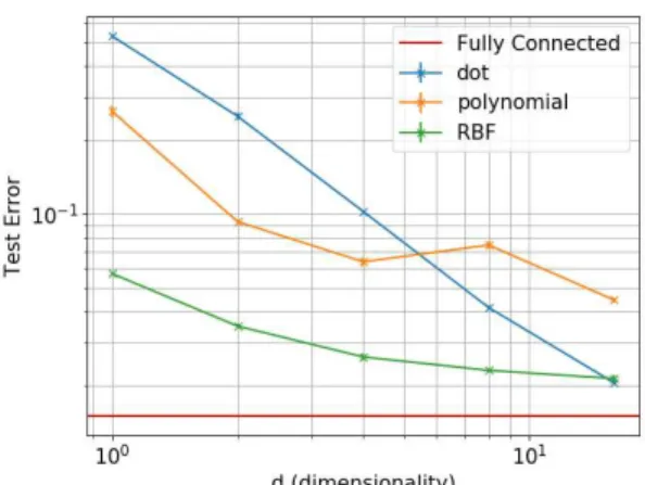
Here we evaluate the performance of three kernelNets of the same structure as a function of the dimensionality𝑑, but using different kernels, whose corresponding embedding 𝜙maps to spaces of different dimensionality𝑑∗. Namely we use a dot-product kernel (embedding dimensionality 𝑑∗ = 𝑑), a second degree polynomial kernel (embedding dimensionality𝑑∗= 1
2(𝑑+ 1)⋅(𝑑+ 2)) and a Gaussian RBF kernel (embedding dimensionality𝑑∗is infinite independent of𝑑).
All networks were trained using the ADAM learning rule and a range of hyperparameters (learning rate and l2 reg-ularization); for each network the best mean performance over 5 repetitions is shown.1
In Figure3we see that kernels, whose corresponding em-bedding function𝜙projects into a higher dimensional space,
1code available in supplement
Figure 3.Comparison of identical kernelNets with different ker-nel functions. Kerker-nels corresponding to higher dimensional em-beddings work better for very low dimensional parametrizations. Errorbars indicate the standard error from five repetitions.
lead to better results for very low dimensional parametriza-tion (low values of 𝑑). At high dimensionality the dot-product kernel (corresponding to the inclusion of a linear layer) catches up, and even slightly overtakes the other ker-nels, probably due to the fact that it is easier to optimize. Notably it is thus more memory efficient to use a higher di-mensional kernel; given some target performance, a higher-order kernel will often achieve it with fewer parameters. In a setting where memory look-ups dominate the computational cost, higher-order kernels are a preferable alternative to the commonly used dot-product kernel in model compression. 3.2. Incorporating Channel Relationships
In some situations the vectors⃗𝑢, ⃗𝑣need not be initialized randomly: If there is a known low-dimensional relationship between the different input channels, it can be beneficial to incorporate such knowledge in the choice of initial⃗𝑢, ⃗𝑣. A concrete example is image data for which there is far greater correlation between nearby pixels than between very distant pixels. This distance-dependent correlation is a use-ful piece of information that can be incorporated into a model. In a kernelNet, this can be achieved by initializing ⃗𝑢, ⃗𝑣on a 2 dimensional grid.
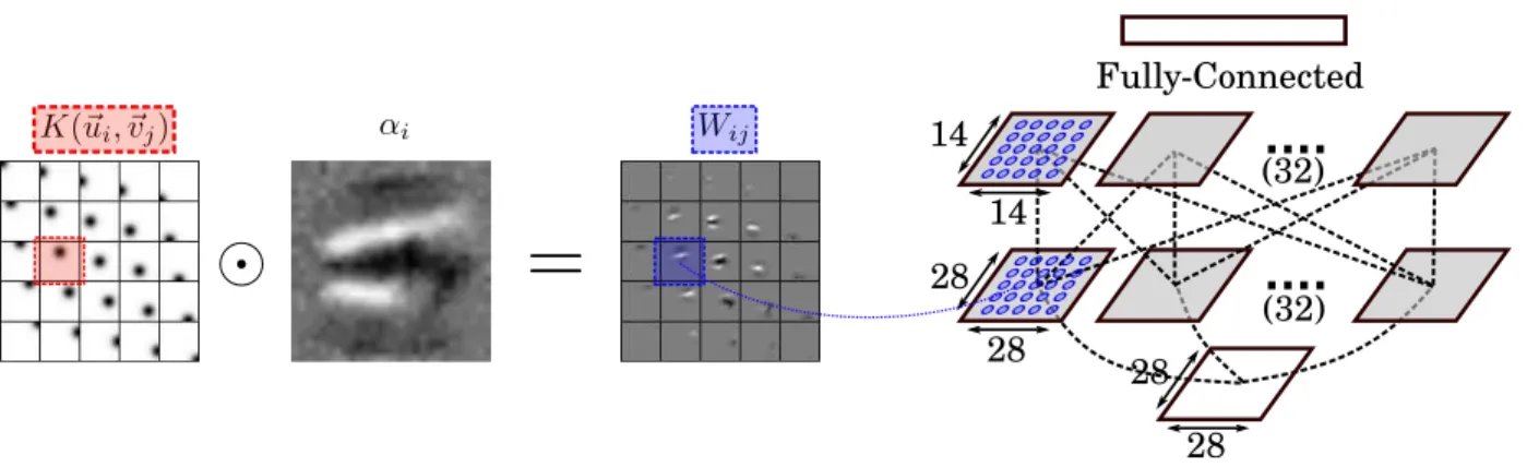
A kernelNet initialized on a 2D grid with a RBF kernel, could be thought of as a convolutional neural network, in which each layer has only a single kernel, but this kernel changes slowly across the image; as a consequence there is no translation equivariance in the kernelNet. See Figure4 for an illustration of receptive fields in the first layer of a network trained on MNIST. With this intuition it becomes apparent that it may be helpful to instantiate several such
....
....
Fully-Connected
14
14
28
28
28
28
(32)
(32)
Figure 4.Architecture of a kernelNet for image classification. Dotted lines indicate 2D RBF kernelized connection matrices, an array of which is visualized on the left. At the bottom an MNIST digit is input, at the top is a fully-connected softmax layer, between are 2D RBF kernelNet-layers, either initialized with or without knowledge of the input pixel locations.
A-priori known pixel-locations Acc.
no 98.89 %
yes 99.03 %
Table 1.Test set classification accuracy on MNIST of the 2-kernelNet in Figure4making use of prior knowledge of pixel locations or not. Adding the prior knowledge improves the perfor-mance. The performance is good for a non-convolutional network trained without data-augmentation.
2D grids in parallel (analogous to having multiple filters in a single layer of a ConvNet), see Figure4for the resulting network architecture.
In Table1we compare the performance of kernelNets using spatial information (by setting the initial⃗𝑢, ⃗𝑣appropriately and keeping them fixed) against the same network lacking this information (randomly initialized ⃗𝑢, ⃗𝑣, trained) in an MNIST classification task. Adding prior information in the architecture indeed improves performance of the network. An interesting consequence of interpretable⃗𝑢𝑖, is that they permit the incorporation of interpretable noise into the net-work: When⃗𝑢𝑖corresponds to a pixel location, adding noise to it can be viewed as a model of uncertainty about the lo-cation of the pixel. This may be beneficial for architectures akin to (Gal & Ghahramani,2016).
3.3. Extensible Data Visualization
In this section we use a kernelNet-layer to create an exten-sible 2D data embedding to create t-SNE-like (Maaten & Hinton,2008) data visualizations.
We build a deep, fully-connected network that contains a single kernelNet-layer in the middle. We choose a 2D RBF-kernel to enforce that neurons in the kernelNet-layer assume a two dimensional spatial organization, and fix the parameters𝑣⃗to lie on a grid (to facilitate visualizations
like in Figure6). Furthermore we equip this layer with the following non-linearity, chosen to ensure sparsity (which in conjunction with the spatial organization of the synaptic matrix leads to spatially unimodal activations)
𝑓(𝑥⃗) = max(0, ⃗𝑥− (𝜂⋅ ̂𝑥+ (1 −𝜂)⋅ ̄𝑥)
)
, (9)
where ̂𝑥is the maximal value of𝑥,⃗ ̄𝑥is its mean value, and 𝜂is an interpolating parameter controlling sparsity (for well-behaved activations this approximates a percentile clipping function). The full network layout is[784 − 2000 − 2000 − 2500 −𝐾1600 − 2000 − 2000 − (10∕784)], where all lay-ers are fully connected, except for the one prefixed with a ‘K’, which is a kernelNet layer (for further details please consult the supplement). From the activations of this layer we construct a 2D embedding of the input: The location to which a particular input to the network is mapped for our data embedding, is the weighted sum of the locations of the hidden units, where the weight is the activation of the unit. We refer to this as the center of mass (𝑐) of that input⃗
⃗ 𝑐= ∑ 𝑖𝑥𝑖𝑣⃗𝑖 ∑ 𝑖𝑥𝑖 (10)
In Figure5we see a 2D map of MNIST digits constructed by such a network trained with two different costs and fi-nal layers: An autoencoder (Bengio et al.,2013) (with per pixel entropy), and a classifier (with categorical cross-entropy). Notably the shown digits are test data and have never been seen by the network. In contrast to e.g. t-SNE (Maaten & Hinton,2008) this method thus is naturally exten-sible beyond the training set (though there exist extenexten-sible variants (van der Maaten,2009)). Furthermore our method distinguishes itself by the fact that the embedding can be based on any cost function. The layers preceding the ker-nelNet layer, learn a mapping from the input space to the latent space sampled (at locations𝑣) by the kernelNet units;⃗ the layers following the embedding layer, learn a mapping
(a)
(b)
Figure 5.Embedding of unseen (test set) MNIST digits using a kernelNet-layer.(a)Trained as an autoencoder (without labels)(b)
Trained as a classifier (with labels). The black, dashed window is also shown in a different representation in Figure6. The left figures show the digits with points placed at their location according to Eq (10) while the right figures show the images of the digits placed at those locations.
Figure 6.Visualization of part of the latent space constructed by the kernelized layer when presented with an artificial, shifted Gaussian input, traveling through the black dashed window in Figure5. Larger Image in supplement.
between the latent space –in which the units of the ker-nelNet layer live– to the output. This second part of the network thus mitigates between the cost-function and the embedding.2
When the whole network is trained as an autoencoder, the decoder part operates as a map from 2D Gaussian kernels (shifted according to Equation (9)) to the space of MNIST digits. Figure6illustrates what digit the decoder constructs, for an artificial, shifted Gaussian input, whose center is slowly translated in the 2D kernelized space. Notably, the network produces sensible outputs at a very fine granularity. From a conceptual point of view, this network shares simi-larities with variational autoencoders (Kingma & Welling, 2013) or adversarial autoencoders (Makhzani et al.,2015) in that it learns the mapping (and its inverse) of a data space to a low dimensional latent space. We encourage a comparison of Figure6with Figure 2 of (Makhzani et al.,2015). In these other works, though the method is different, coordinates in the latent 𝑑-dimensional space are explicitly represented by a layer with𝑑units; these units are constrained by an additional cost term, to sample from a desired distribution. In this work, we use the structural constraint of a weight matrix lying in a low dimensional kernel space to achieve a similar outcome.
3.4. Pre-trained Network Visualization
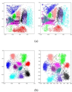
Here we visualize the action of a pre-trained network (a convolutional ResNet (He et al.,2016)) by copying it up to some prespecified depth and adding on top a fully-connected layer (with 500 units), a 2D-RBF kernelNet-layer (with 900 units) and a classification layer (a 10-way softmax). We then train the newly appended part of this truncated network with the same cost as the original network and visualize the activation in the embedding layer as described in the previous section (the lower part of the network remains unchanged)
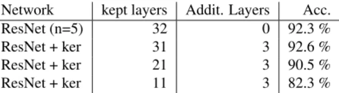
Note that the embedding layers are trained to optimize the same cost (categorical cross-entropy) as the original net-work. Indeed the output of the embedding layer is suffi-ciently informative to reach an equally good (or slightly better) classification as the original network (see Table2). The resulting embeddings (created as in the previous sec-tion) are shown in Figure7.
These visualizations contain similar information as a confu-sion matrix would, but more intuitively presented, showing how well the various classes are separated from each other. Figure7shows how the classes overlap increasingly more, as we visualize the network action for lower layers.
(a) (b) (c)
Figure 7.(a)Embedding of test-set CIFAR-10 images created by an RBF Kernelized layer stacked onto a CIFAR-10 pre-trained, 51-layer ResNet without the final classification layer(b)like previous, but the last 11 layers of the ResNet were removed(c)last 21 layers removed [Best viewed in color]
Network kept layers Addit. Layers Acc.
ResNet (n=5) 32 0 92.3 %
ResNet + ker 31 3 92.6 %
ResNet + ker 21 3 90.5 %
ResNet + ker 11 3 82.3 %
Table 2.Classification performance of the pre-trained truncated ResNets used for the visualizations in Figure7.
3.5. Recommender Systems
Recommender systems typically operate on sparse high-dimensional data. For instance, one aims at predicting movie ratings for a user based on millions of other users having each seen a small subset of thousands of movies (Lam & Herlocker,2012). In such settings, it is a common assump-tion that the sparsely observed matrix entries, from which one ought to generalize, can in some way be represented in a low dimensional space. Indeed, movie-ratings supposedly correlate with a relatively small number of features: the combination of an actor playing in it and a movie genre for example. As data is expected to be best explained by such a low dimensional model it seems this is a well-suited setting for kernelNets.
3.5.1. DATASET
We train our models to predict movie ratings of the MovieLens-10M (ML-10M), MovieLens-1M (ML-1M) and MovieLens-100K (ML-100K) datasets (Harper & Konstan, 2016). These datasets comprise (10 million / 1 million / 100 thousand) ratings of (10681 / 3706 / 1700) movies by ca. (71 / 16 / 1) thousand users respectively, on a scale of𝑟 ∈ {1,2,3,4,5}(ML-10M include half ratings). The datasets are highly sparse (density 0.013 / 0.045 / 0.059). We randomly designate10%or20%respectively of the given
ratings as validation data (so chosen to match the models we compare to). The validation data is not used in training and used alone in the reported error computation. Reported performances average over five such random splits. We report the root-mean-square error (Equation (11)).
𝐸𝑟𝑚𝑠𝑒=√∑
𝑖
(𝑝𝑖−𝑟𝑖)2∕𝑁, (11) where𝑝𝑖 is the predicted rating,𝑟𝑖 is the true rating. 𝑁is
the number of validation samples. 3.5.2. MODEL
Our model is an item-based autoencoder very similar to (Sedhain et al.,2015), but the weight matrices𝐖,𝐕are
reparameterized. Firstly we use a kernelNet-Layer with the following kernel (which is not positive semi-definite, but works well in practice)
𝐾𝜎(⃗𝑢, ⃗𝑣) =tanh(⃗𝑢⋅𝑣⃗) (12) secondly we use the Hadamard-product of a dense connec-tion matrix with a kernelized weight matrix, with finite-support kernel (as in Eq. (7)), to obtain sparse connection matrices. The full model then is
ℎ(⃗𝑟, 𝜃) =𝑓(𝐖 ⋅𝑔 ( 𝐕⃗𝑟+𝜇⃗)+⃗𝑏 ) (13) where the weight matrices either take the form
𝑉𝑖𝑗 = 𝛼𝑖𝐾𝜎(𝑣⃗𝑖, ⃗𝑢𝑗) (14) 𝑊𝑖𝑗 = 𝛽𝑖𝐾𝜎(⃗𝑠𝑖, ⃗𝑡𝑗). (15) or the form using𝐾fs(defined in Eq. (7)), that we will refer to as ‘sparse fully-connected’:
𝑉𝑖𝑗 = 𝛼𝑖𝑗𝐾fs(𝑣⃗𝑖, ⃗𝑢𝑗) (16)
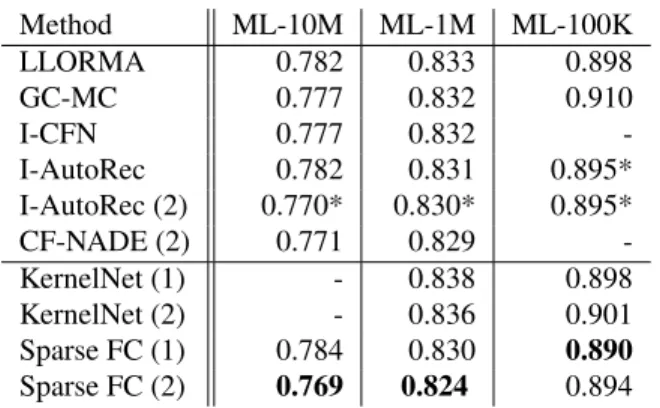
Method ML-10M ML-1M ML-100K LLORMA 0.782 0.833 0.898 GC-MC 0.777 0.832 0.910 I-CFN 0.777 0.832 -I-AutoRec 0.782 0.831 0.895* I-AutoRec (2) 0.770* 0.830* 0.895* CF-NADE (2) 0.771 0.829 -KernelNet (1) - 0.838 0.898 KernelNet (2) - 0.836 0.901 Sparse FC (1) 0.784 0.830 0.890 Sparse FC (2) 0.769 0.824 0.894
Table 3.Comparison of various methods on MovieLens tasks; the mean RMSE of the predicted ratings is given (lower is better) in our case from five CV folds (Sparse FC std. err. < 0.0005for ML-1M, ML-10M and<0.005for ML-100K), training validation split 90/10 (ML-1M, ML-10M) and 80/20 (ML-100K). Numbers in brackets indicate number of hidden layers used. Architectures from this work follow the second horizontal line. *Our implementation.
As in (Sedhain et al.,2015) for optimization we use the L-BFGS-B (Zhu et al.,1997) and RPROP (Riedmiller & Braun,1993) optimizers to minimize a regularized square-error, the regularization term added to the cost is
𝑅=𝜆2 ( 𝑊2 𝑖𝑗+𝑉𝑖𝑗2 ) , and in the sparse fully-connected case
𝑅=𝜆2 ( ∑ 𝑖𝑗 𝛼𝑖𝑗+∑ 𝑖𝑗 𝛽𝑖𝑗 ) +𝜆0 ( ∑ 𝑖𝑗 𝐾(𝑣⃗𝑖, ⃗𝑢𝑗) +∑ 𝑖𝑗 𝐾(⃗𝑠𝑖, ⃗𝑡𝑗) ) ,
One may think of𝜆2as the𝐿2regularization and𝜆0as the sparsity “𝐿0” regularization parameters. For the kernelNet we use𝑑= 50and for the sparse fully-connected case𝑑= 5. All hidden layers have size 500.3
3.5.3. RESULTS
In Table3we report the mean validation RMSE of 5 runs in which each time a randomly drawn10%of the ML-1M and ML-10M dataset and20%of the ML-100K dataset were used as validation data and compare to the following meth-ods: LLORMA (Lee et al.,2016), GC-MC (van den Berg et al.,2017), I-CFN (Strub et al.,2016), I-AutoRec (Sedhain et al.,2015) and CF-NADE (Zheng et al.,2016). We cite the performance of the models trained without information outside ratings (such as movie genres, user age, etc.) as we did not use such information either.
Table 4 further shows comparisons and highlights the gained efficiency in terms of multiply-accumulate
opera-3Code available in the supplement.
Method Parameters MACs ML-1M
I-AutoRec (1) 6.05 M 3.03 M 0.831 I-AutoRec (2) 6.30 M 3.28 M 0.830 I-KernelNet (1) 0.67 M 3.03 M 0.838 I-KernelNet (2) 0.72 M 3.28 M 0.836 Sparse FC (1) 6.70 M 2.77 M 0.830 Sparse FC (2) 7.00 M 2.23 M 0.824 Table 4.Here we highlight how the two proposed reparameteri-zations reduce the number of free parameters (KernelNet) or the expected number of MACs required (Sparse FC) for a prediction (assuming 10 random rated Movies and dense prediction on ML-1M).
tions (MACs) (i.e. lower number of non-zero entries in the weight matrix) thanks to the here proposed parameterization. The parameter𝜆0allows trading-off Number of MACs for performance; the table shows the best performing model. Our model (Sparse FC (2)) shows state-of-the-art perfor-mance, while decreasing the number of MACs required for its evaluation by ca30%compared to fully-connected, unal-tered I-AutoRec model. The performance gain is especially pronounced for the intermediate size dataset.
4. Conclusion
We presented a novel neural network layer structure, based on kernel-approximations of the synaptic weight matrix. We detailed the mathematical relationship of the proposed kernelNet to standard fully-connected layers. Furthermore we demonstrated state-of-the-art performance on various MovieLens datasets (in terms of generalization MSE), us-ing an Autoencoder whose weight matrices were sparsified using finite-support kernels, which additionally decreased the computational cost at inference in terms of multiply-accumulate operations. Finally we gave some illustrative examples with further possible applications, including a natively extensible data visualization technique that can be trained to reflect any cost function. KernelNets give a new approach to imposing structure on neural networks, regularizing and sparsifying them and for making the in-ner workings – also of pretrained networks – more easily interpretable.
Acknowledgements
We acknowledge funding by the Swiss National Science Foundation under grant number CRSII2_160756. We thank the NCS and CO2groups at the Institute of Neuroinformat-ics for helpful discussions, and we thank the reviewers for their work and their insightful comments.
References
Bengio, Y., Courville, A., and Vincent, P. Representation learning: A review and new perspectives. IEEE
transac-tions on pattern analysis and machine intelligence, 35(8):
1798–1828, 2013.
Denil, M., Shakibi, B., Dinh, L., de Freitas, N., et al. Predict-ing parameters in deep learnPredict-ing. InAdvances in Neural
Information Processing Systems, pp. 2148–2156, 2013.
Fernando, C., Banarse, D., Reynolds, M., Besse, F., Pfau, D., Jaderberg, M., Lanctot, M., and Wierstra, D. Convolution by evolution: Differentiable pattern producing networks.
InProceedings of the 2016 on Genetic and Evolutionary
Computation Conference, pp. 109–116. ACM, 2016.
Gal, Y. and Ghahramani, Z. Dropout as a bayesian approx-imation: Representing model uncertainty in deep learn-ing. Ininternational conference on machine learning, pp. 1050–1059, 2016.
Gomez, F. and Schmidhuber, J. Evolving modular fast-weight networks for control.Artificial Neural Networks:
Formal Models and Their Applications–ICANN 2005, pp.
750–750, 2005.
Ha, D., Dai, A., and Le, Q. V. Hypernetworks. arXiv
preprint arXiv:1609.09106, 2016.
Harper, F. M. and Konstan, J. A. The movielens datasets: History and context. ACM Transactions on Interactive
Intelligent Systems (TiiS), 5(4):19, 2016.
He, K., Zhang, X., Ren, S., and Sun, J. Deep residual learn-ing for image recognition. InProceedings of the IEEE
Conference on Computer Vision and Pattern Recognition,
pp. 770–778, 2016.
Ioffe, S. and Szegedy, C. Batch normalization: Accelerating deep network training by reducing internal covariate shift.
InInternational Conference on Machine Learning, pp.
448–456, 2015.
Jaderberg, M., Vedaldi, A., and Zisserman, A. Speeding up convolutional neural networks with low rank expansions.
arXiv preprint arXiv:1405.3866, 2014.
Kingma, D. P. and Welling, M. Auto-encoding variational bayes.arXiv preprint arXiv:1312.6114, 2013.
Klambauer, G., Unterthiner, T., Mayr, A., and Hochreiter, S. Self-normalizing neural networks. InAdvances in Neural
Information Processing Systems, pp. 972–981, 2017.
Koutnik, J., Gomez, F., and Schmidhuber, J. Evolving neural networks in compressed weight space. InProceedings of the 12th annual conference on Genetic and evolutionary
computation, pp. 619–626. ACM, 2010.
Krogh, A. and Hertz, J. A. A simple weight decay can im-prove generalization. InAdvances in neural information
processing systems, pp. 950–957, 1992.
Lam, S. and Herlocker, J. Movielens 1m dataset, 2012. Lee, J., Kim, S., Lebanon, G., Singer, Y., and Bengio, S.
Llorma: Local low-rank matrix approximation. The
Jour-nal of Machine Learning Research, 17(1):442–465, 2016.
Maaten, L. v. d. and Hinton, G. Visualizing data using t-sne. Journal of Machine Learning Research, 9(Nov): 2579–2605, 2008.
Makhzani, A., Shlens, J., Jaitly, N., Goodfellow, I., and Frey, B. Adversarial autoencoders. arXiv preprint
arXiv:1511.05644, 2015.
Moczulski, M., Denil, M., Appleyard, J., and de Freitas, N. Acdc: A structured efficient linear layer.arXiv preprint
arXiv:1511.05946, 2015.
Riedmiller, M. and Braun, H. A direct adaptive method for faster backpropagation learning: The rprop algorithm. In
Neural Networks, 1993., IEEE International Conference on, pp. 586–591. IEEE, 1993.
Sainath, T. N., Kingsbury, B., Sindhwani, V., Arisoy, E., and Ramabhadran, B. Low-rank matrix factorization for deepneuralnetworktrainingwithhigh-dimensionalout-put targets. InAcoustics, Speech and Signal Processing
(ICASSP), 2013 IEEE International Conference on, pp.
6655–6659. IEEE, 2013.
Schmidhuber, J. Discovering neural nets with low kol-mogorov complexity and high generalization capability.
Neural Networks, 10(5):857–873, 1997.
Scholkopf, B. and Smola, A. J. Learning with kernels: support vector machines, regularization, optimization,
and beyond. MIT press, 2001.
Sedhain, S., Menon, A. K., Sanner, S., and Xie, L. Autorec: Autoencoders meet collaborative filtering. InProceedings
of the 24th International Conference on World Wide Web,
pp. 111–112. ACM, 2015.
Srivastava, N., Hinton, G., Krizhevsky, A., Sutskever, I., and Salakhutdinov, R. Dropout: A simple way to prevent neural networks from overfitting.The Journal of Machine
Learning Research, 15(1):1929–1958, 2014.
Stanley, K. O., D’Ambrosio, D. B., and Gauci, J. A hypercube-based encoding for evolving large-scale neural networks. Artificial life, 15(2):185–212, 2009.
Strub, F., Gaudel, R., and Mary, J. Hybrid recommender system based on autoencoders. InProceedings of the 1st
Workshop on Deep Learning for Recommender Systems,
Tai, C., Xiao, T., Zhang, Y., Wang, X., et al. Convolutional neural networks with low-rank regularization. arXiv
preprint arXiv:1511.06067, 2015.
van den Berg, R., Kipf, T. N., and Welling, M. Graph convolutional matrix completion.stat, 1050:7, 2017. van der Maaten, L. Learning a parametric embedding by
preserving local structure.RBM, 500(500):26, 2009. Zheng, Y., Tang, B., Ding, W., and Zhou, H. A neural
autoregressive approach to collaborative filtering. In Pro-ceedings of the 33rd International Conference on
Interna-tional Conference on Machine Learning-Volume 48, pp.
764–773. JMLR. org, 2016.
Zhu, C., Byrd, R. H., Lu, P., and Nocedal, J. Algorithm 778: L-bfgs-b: Fortran subroutines for large-scale bound-constrained optimization.ACM Transactions on