Bootstrapping Cointegrating Regressions

Yoosoon Chang

Department of Economics Rice University

Joon Y. Park

School of Economics Seoul National University

Kevin Song

Department of Economics Yale University

Abstract

In this paper, we consider bootstrapping cointegrating regressions. It is shown that the method of bootstrap, if properly implemented, generally yields con-sistent estimators and test statistics for cointegrating regressions. We do not assume any speci¯c data generating process, and employ the sieve bootstrap based on the approximated ¯nite-order vector autoregressions for the regression errors and the ¯rst di®erences of the regressors. In particular, we establish the bootstrap consistency for OLS method. The bootstrap method can thus be used to correct for the ¯nite sample bias of the OLS estimator and to approximate the asymptotic critical values of the OLS-based test statistics in general cointegrat-ing regressions. The bootstrap OLS procedure, however, is not e±cient. For the e±cient estimation and hypothesis testing, we consider the procedure proposed by Saikkonen (1991) and Stock and Watson (1993) relying on the regression aug-mented with the leads and lags of di®erenced regressors. The bootstrap versions of their procedures are shown to be consistent, and can be used to do inferences that are asymptotically valid. A Monte Carlo study is conducted to investigate the ¯nite sample performances of the proposed bootstrap methods.

This version: February 18, 2002

Key words and phrases: cointegrating regression, sieve bootstrap, e±cient estimation and hypothesis testing, AR approximation.

1

Park thanks the Department of Economics at Rice University, where he is an Adjunct Professor, for its continuing hospitality and secretarial support. Correspondence address to: Yoosoon Chang, Department of Economics, Rice University, 6100 Main Street, Houston, TX 77005-1892, Tel: 2796, Fax: 713-348-5278, Email: [email protected].

1. Introduction

The bootstrap has become a standard tool for the econometric analysis. Roughly, the pur-pose of using the bootstrap methodology is twofold: To ¯nd the distributions of statistics whose asymptotic distributions are unknown or dependent upon nuisance parameters, and to obtain re¯nements of the asymptotic distributions that are closer to the ¯nite sample distributions of the statistics. It is well known that the bootstrap statistics have the same asymptotic distributions as the corresponding sample statistics for a very wide, if not all, class of models, and therefore, the unknown or nuisance parameter dependent limit distribu-tions can be approximated by the bootstrap simuladistribu-tions. Moreover, if properly implemented to pivotal statistics, the bootstrap simulations indeed provide better approximations to the ¯nite sample distributions of the statistics than their asymptotics. See Horowitz (2002) for an excellent nontechnical survey on the subject.

The purpose of this paper is to develop the bootstrap theory for cointegrating regres-sions. The bootstrap can be potentially more useful for models with nonstationary time series than for the standard models with stationary time series, since the statistical theories for the former are generally nonstandard and depend, often in a very complicated manner, upon various nuisance parameters. Nevertheless, the bootstrap theories for the former are much less developed compared to those for the latter. Virtually all of the published works on the theoretical aspects of the nonstationary bootstrap consider simple unit root models. See, e.g., Basawa et al. (1991), Chang (2000), Chang and Park (2002b) and Park (2000, 2002). The bootstrap cointegrating regression has been studied only by simulations as in Li and Maddala (1997). The bootstrap method, however, is used quite frequently and ex-tensively by empirical researchers to approximate the distributions of the statistics in more general models with nonstationary time series.

We consider the sieve bootstrap to resample from the cointegrating regressions. The method does not assume any speci¯c data generating processes, and the data are simply ¯tted by a VAR of order increasing with the sample size. The bootstrap samples are then constructed using the ¯tted VAR from the resampled innovations. We show in the paper that under such a scheme the bootstrap becomes consistent for both the usual OLS and the e±cient OLS by Saikkonen (1991) and Stock and Watson (1993). The sieve bootstrap can therefore be used to reduce the ¯nite sample bias of the OLS estimator, and also to ¯nd the asymptotic critical values of the tests based on the OLS estimator. The bootstrapped OLS estimator, however, is ine±cient just as is the sample OLS estimator. The bootstrap does not improve the e±ciency. To attain e±ciency, we need to bootstrap the e±cient OLS estimator. The sieve bootstrap can be naturally implemented to do resampling for the e±cient estimator, which itself relies on the idea of sieve estimation of the cointegrating regression. We show in the paper that the sieve bootstrap is generally consistent for the e±cient OLS method.

Though we focus on the prototype multivariate cointegration model in the paper for concreteness, the theory we derive here can be used to analyze more general cointegrated models. The immediate extensions are the cointegrating regressions with more °exible de-terministic trends including those allowing for structural breaks. Cointegrating regressions with shifts in the coe±cients can also be analyzed using the methods developed in the paper.

Moreover, our theory extends further to the cointegrating regressions represented as error correction models, seemingly unrelated cointegrated models and panels with cointegration in individual units. The sieve bootstrap proposed here can be applied to all such models only with some obvious modi¯cations. The estimation of and testing for the cointegration parameters can therefore be performed or re¯ned by the sieve bootstrap. It is well expected that the sieve bootstrap is consistent for the aforementioned models if implemented properly as suggested in the paper, and it can be proved rigorously, if necessary, using the theory established in the paper.

The rest of the paper is organized as follows. Section 2 introduces the model, assump-tions and some preliminary results. The multivariate cointegrating regression with a detailed speci¯cation for data generating process is given, and a strong invariance principle, which can be used for both the sample and bootstrap asymptotics, is introduced and discussed. The standard asymptotic results for the cointegrating regressions are then derived. In Sec-tion 3, the sieve bootstrap procedure is presented, and the relevant bootstrap asymptotics are developed. The bootstrap consistency is established there. Section 4 summarizes our simulation study, and Section 5 concludes the paper. All the mathematical proofs are given in Section 6.

A word on notation. Following the standard convention, we use the superscript \¤" to signify whatever is related to the bootstrap samples and dependent upon the realization of the samples. The usual notations for the modes of convergence such as!a:s:,!pand!dare used without additional references, and the notation =ddenotes the equality in distribution. The stochastic order symbols op and Op are also used frequently. Moreover, we often use such standard notations with the superscript \¤" to imply their bootstrap counterparts. We use the notationj ¢ j to denote the Euclidean norm for vectors and matrices, i.e.,jxj2 _=x0_x and jAj2 _{= trA}0_{A for a vector x and a matrix A. For matrices, we also use the operator} normk¢k, i.e.,kAk= maxxjAxj=jxjfor a vectorxand a matrixAwhich are of conformable dimensions. For a matrix A, vec(A) denotes a column vector which stacks row vectors of A.

2. The Model, Assumptions and Preliminary Results

2.1 The Model and Assumptions

We consider the regression model given by

yt = ¦0xt+ut (1)

xt = xt¡1+vt fort= 1;2; : : :, where

wt= (u0t; v0t)0

is an (`+m)-dimensional stationary vector process. Under this speci¯cation, the model introduced in (1) becomes a multivariate cointegrating regression. For the subsequent de-velopment of our theory, we letx0 be any random variable which is stochastically bounded,

and let (wt) be a linear process given by wt= ª(L)"t (2) where ª(z) = 1 X k=0 ªkzk We make the following assumptions.

Assumption 2.1 We assume

(a) ("t) are iid random variables such that E"t = 0, E"t"0

t = § >0 and Ej"tja < 1 for

some a¸4.

(b) det ª(z)6= 0for all jzj ·1,and P1k=0jkjbjªkj<1for some b¸1 .

The conditions in Assumption 2.1 are not necessary for our results in this section. In particular, the iid assumption on the innovation ("t) is not required. It is introduced here just to make our forthcoming bootstrap procedure more meaningful. All the subsequent theoretical results may be obtained under weaker martingale di®erence assumptions on ("t). Also, 1-summability of (ªk) is assumed to simplify the proofs, and can be weakened to 1=2-summability. Yet, a wide class of cointegrated models, including Gaussian error correction models considered in Johansen (1988, 1991), can be represented as the model speci¯ed in (1) and (2) with ("t) and (ªk) satisfying the conditions in Assumption 2.1.

2.2 Invariance Principles

For the iid random vectors ("t), we de¯ne

Wn(r) =dn¡1=2 [nr]

X

t=1 "t

Then the invariance principle for the iid random vectors ("t) holds, i.e.,

Wn!dW (3)

whereW is a vector Brownian motion with variance §. In particular, we have

Lemma 2.2 Let Ej"tja<1 for some a >2. Then we may de¯ne on a common proba-bility space Wn and W such that

P ( sup 0·r·1jWn(r)¡W(r)j> n ¡1=2_cn ) ·Kn c¡naEj"tja

for any numerical sequence (cn), cn = n1=a+± _{for some ± > 0, where K is an absolute}

Lemma 2.2 follows immediately from the strong approximation result established in Einmahl (1987). For any givena >2, we may choose± such that 0< ± <1=2¡1=ato show

sup

0·r·1jWn(r)¡W(r)j=op(1)

and therefore, the invariance principle (3) follows directly from Lemma 2.2. The use of strong approximation for the proof of the invariance principle (3) is very useful in our context, since it can also be directly applied to derive the corresponding invariance principle for the bootstrap samples. This will be shown in the next section.

The invariance principle for ("t) directly carries over to the one for (wt). We have from the Beveridge-Nelson decompostion that

wt= ª(1)"t+ ( ¹wt¡1¡wt)¹ with ¹wt=P1_k=0ª¹k"t¡k and ¹ªk=P1i=k+1ªi, and therefore,

Bn(r) = n¡1=2 [nr] X t=1 wt = n¡1=2ª(1) [nr] X t=1 "t+n¡1=2( ¹w0¡w¹[nr]) = ª(1)Wn(r) +Rn(r) (4) where sup 0·r·1jRn(r)j=op(1)

since ( ¹wn) is well-de¯ned and stationary under our 1-summability condition on (ªk). The reader is referred to Phillips and Solo (1992) for more details. It now follows immediately from (4) that

Bn!dB (5)

whereB is an (`+m)-dimensional vector Brownian motion with variance - = ª(1)§ª(1)0. We call - the longrun variance of (wt). If we let ¡(k) = Ewtw_t0_+k be the autocovariance function of (wt), then we may de¯ne the longrun variance of (wt) as - = P1k=¡1¡(k). Correspondingly, we denote by ¢ the one-way longrun variance ofwt, i.e., ¢ =P1_k=0¡(k). We letB= (B10; B20)0 and partition - = (-ij) and ¢ = (¢ij) into cell matrices fori; j= 1;2, conformably withwt= (u0t; vt)0.

2.3 Inference on Parameters

As is well known, the parameter ¦ in the multivariate cointegrating regression (1) can be consistently estimated by the OLS estimator ^¦n, whose limiting distribution is given by

n( ^¦n¡¦)!d µZ 1 0 B2B 0 2 ¶¡1µZ ₁ 0 B2dB 0 1+ ¢21 ¶

as n! 1. Though the OLS estimator ^¦n is super-consistent, it is asymptotically biased and ine±cient when (ut) and (vt) are correlated. Moreover, the tests based on the OLS estimator ^¦n are generally invalid. For the test of the hypothesis

H0: ¸(¦) = 0 (6)

where¸:R`m!R·is continuously di®erentiable with ¯rst-order derivative ¤ =@¸=@¼0; ¼= vec ¦, we may consider the Wald-type statistic

^

Tn= ^¸0_n³¤n(M^ _n¡1--11) ^¤0n

´¡1_^

¸n (7)

where ^¸n=¸( ^¦n), ^¤n= ¤( ^¦n) andMn=Pnt=1xtx0t. For the practical implementation, of course, the longrun variance -11 of (ut) must be estimated. The statistic has the limiting distribution

^

Tn!d¿0Q¡1¿ (8)

where ¿ = ¤(M¡1-I`)(R₀1B2-dB1+±21) and Q= ¤(M¡1--11)¤0 using the notations ¤ = ¤(¦), ±21 = vec ¢21 and M = R01B2B20. The asymptotic distribution of Tn is thus nonstandard and dependent upon various nuisance parameters. See, e.g., Park and Phillips (1988) for the distribution theories for ^¦n and ^Tn.

For the e±cient estimation of ¦, we consider the procedure suggested by Saikkonen (1991) and Stock and Watson (1993), which is based on the regressions augmented with the leads and lags of the ¯rst-di®erenced regressors4xt. Under Assumption 2.1, we may write

ut= 1

X

k=¡1

¦0_kvt_¡k+´t (9)

where (´_t) is uncorrelated with (vt) = (4xt) at all leads and lags with variance -11¢2 = -11¡-12-¡221-21, and P1k=¡1j¦kj<1. The reader is referred to Saikkonen (1991) and the references cited therein for the representation in (9).

We are therefore led to consider the regression yt= ¦0xt+ X

jkj·p

¦0k4xt¡k+´pt (10)

where´pt=´t+Pjkj>p¦0k4xt¡k. Since (¦k) are absolutely summable, we may well expect that the error (´_pt) will become close to (´_t) if we let the number p of included leads and lags of the di®erenced regressors increase appropriately as the sample sizengrows. Indeed, Saikkonen (1991) shows that if we letp! 1such thatp3=n!0 andn1=2P_jkj>pj¦kj !0, then the regression (10) is asymptotically equivalent to

yt= ¦0xt+´t (11)

In particular, the OLS estimator ~¦nof ¦ in regression (10), which we call the e±cient OLS estimator, has the asymptotics given by

n( ~¦n¡¦)!d µZ 1 0 B2B 0 2 ¶¡1Z ₁ 0 B2d(B1¡-12 -¡1 22B2)0 (12)

which is precisely the same as the asymptotics of the OLS estimator of ¦ from regression (11).

Note that B1¡-12-¡₂₂1B2 has reduced variance -11¢2 = -11¡-12-¡₂₂1-21 relative to the variance -11ofB1. The asymptotic variance of ~¦nis therefore smaller than that of ^¦n. Moreover,B1¡-12-¡122B2 is independent ofB2, and consequently the limiting distribution of ~¦n is mixed normal, which is quite a contrast to the nonstandard limit theory of ^¦n. As a result, the usual chi-square test is valid if we use a test statistic based on ~¦n. Indeed, for testing the hypothesis (6), we may use

~ Tn= ~¸0n ³ ~ ¤n(Mnn¡1--11¢2)~¤0n ´¡1 ~ ¸n (13)

where ~¸n = ¸( ~¦n) and ~¤n = ¤( ~¦n) are de¯ned similarly as ^¸n and ^¤n introduced in (7), and Mnn is the matrix de¯ning the sample covariance of ~¦n, which corresponds toMn for

^

¦n given also in (7). Then it follows that ~

Tn!dÂ2· (14)

As before, -11¢2 should be consistently estimated for practical applications.

In what follows, we reestablish the asymptotics for the augmented regression (10) using a weaker condition on the expansion rate for p, relative to the one required by Saikkonen (1991). We assume

Assumption 2.3 Let p! 1 and p=o(n1=2_{) as n! 1.}

Our condition on p is substantially weaker than the one used in Saikkonen (1991). Our upper bound for p is extended to o(n1=2) compared to his o(n1=3). Moreover, we do not impose any restriction on the minimum rate at which p must grow. Thus we may allow for the logarithmic rate that is usually imposed for the common order selection rules such as AIC and BIC. The logarithmic rate, however, is not allowed in Saikkonen (1991) unless (¦k) decreases at a geometric rate. The rate for p here is therefore valid for more general stationary process (wt), as can be seen clearly in our proof for the following lemma. Lemma 2.4 Under Assumptions 2.1 and 2.3,we have (12) and (14) as n! 1.

The asymptotics established in the above lemma will be used as a basis for the subsequent development of our bootstrap asymptotics.

3. Bootstrap Procedures and Their Asymptotics

3.1 Bootstrap Procedures

In this section, we introduce the bootstrap procedures for our cointegrating regression model (1) and develop their asymptotics. For our bootstrap procedures introduced below, we may

use various consistent estimates for ¦. Therefore, we use the generic notation ¦nto denote any estimate of ¦ that is n-consistent. More explicitly, we let

¦n= ^¦n;¦n;~ ¦0

where ^¦n and ~¦n are the OLS estimators of ¦ in regressions (1) and (10), respectively, and ¦0 denotes the hypothesized or estimated value of ¦ under the restriction given by the hypothesis (6). Other estimates of ¦, which are asymptotically equivalent to any of these estimators, can also be used.

The cointegrating regression model (1) with the speci¯cation (2) of its stationary com-ponent as a linear process can be bootstrapped using the standard sieve method. The method of sieve bootstrap requires to ¯t the linear process (wt) to a ¯nite order VAR with the order increasing as the sample size grows. We may rewrite (wt) as a VAR

©(L)wt="t

with ©(z) = I¡P1k=1©kzk, since ª(L) in (2) is invertible, and therefore it is reasonable to approximate (wt) as a ¯nite order VAR

wt= ©1wt¡1+¢ ¢ ¢+ ©qwt¡q+"qt (15) with"qt="t+P_jkj>q©kwt¡k. The orderq of the approximated VAR is set to increase at a controlled rate ofn, as we will specify below. In practice, it can be chosen by one of the commonly used order selection rules such as AIC and BIC.

Assumption 3.1 Let q! 1 andq =o(n1=2_{) as n! 1.}

The required condition on the expansion rate for q in Assumption 3.1 is identical to that forp given in Assumption 2.3.

Outlined below are the necessary steps for obtaining the bootstrap samples (x¤_t) and (yt¤) for (xt) and (yt), respectively.

Step 1: Fit regression (1) to obtain (^ut), i.e., yt= ¦0_nxt+ ^ut and de¯ne ^wt = (^u0

t; vt0)0, where vt = 4xt. As mentioned above, we may use various estimates ¦n of ¦ here.

Step 2: Apply the sieve estimation method to the VAR (15) of ( ^wt) to get the ¯tted values (^"qt) of ("qt), i.e.,

^

wt= ^©1wt^¡1+¢ ¢ ¢+ ^©qwt^¡q+ ^"qt (16) Obtain ("¤_t) by resampling the centered ¯tted residuals

à ^ "qt¡ 1 n n X t=1 ^ "qt !n t=1

and construct the bootstrap samples (w¤t) recursively using wt¤= ^©1wt¤¡1+¢ ¢ ¢+ ^©qwt¤¡q+"¤t

given the initial values w_t¤ =wt for t= 0; : : : ;1¡q. This step amounts to the usual sieve bootstrap for ( ^wt).

Step 3: De¯ne wt¤ = (u¤0t; v¤0t )0 analogously as wt= (u0t; vt0)0. Obtain the boot-strap samples (x¤_t) by integrating (v_t¤), i.e., x¤_t = x¤₀+Pt_k=1v¤_t, with x¤₀ = x0 and generate the bootstrap samples (y¤_t) from

y_t¤ = ¦0_nx¤_t +u¤_t

The estimate ¦n of ¦ here need not be the same as the one used in Step 1.

The bootstrap samples (x¤_t) and (y_t¤) can be used to simulate the distributions of various statistics as explained below.

Discussions on some practical issues arising from the implementation of our bootstrap method are in order. First, the choice of an estimator ¦n for ¦ should be made in Steps 1 and 3. The choice in Step 3 is not important, as long as we regard the chosen estimate as the true parameter for the bootstrap samples. The choice of ¦n for ¦ we use in Step 1, however, is very important, as it would a®ect the subsequent bootstrap procedure in Steps 2 and 3. In particular, the order selection rule applied to determine the model in Step 2 can be very sensitive to the choice of ¦n made in Step 1. Naturally, we recommend to use the best possible estimate, i.e., the most e±cient estimate available incorporating all restrictions for the hypothesis testing. This is what is observed by Chang and Park (2002b) for the bootstrap unit root tests. Li and Maddala (1997) also ¯nd that using the true value in Step 1 yields the best result for the bootstrap hypotheses tests. Second, the initializations for the generations of (w¤

t) and (x¤t) are necessary respectively in Steps 2 and 3. The choices w¤t =wtfort= 0; : : : ;1¡qand x¤0 =x0 make the results conditional on these initial values of the samples. To reduce or eliminate such dependencies, we may generate su±ciently large number of (w¤

t) and retain only last ndrawings, or include a constant so that the estimate ¦n of ¦ is independent of the initial value of (x¤t).

We consider the bootstrap version of regression (1) given as

yt¤ = ¦0nx¤t +u¤t (17) which yields the bootstrap estimator for the usual OLS, viz.,

^ ¦¤_n= à _n X t=1 x¤_tx¤0_t !¡1Ã_Xn t=1 x¤_ty_t¤0 !

We also look at the bootstrap version of regression (10), which we write as yt¤ = ¦0nx¤t +

X

jkj·p

where

´¤_pt= X jkj>p

¦¤0_kv_t¤_¡k+´¤_t

The e±cient bootstrap OLS estimator, i.e., the OLS estimator from regression (18), is given by ~ ¦¤_n= 0 @ n X t=1 x¤_tx¤0_t ¡ à _n X t=1 x¤_tv_pt¤0 ! à _n X t=1 v¤_ptv_pt¤0 !¡1Ã_Xn t=1 v_pt¤x¤0_t !1 A ¡1 ¢ 0 @ n X t=1 x¤tyt¤0¡ à _n X t=1 x¤tvpt¤0 ! à _n X t=1 vpt¤vpt¤0 !¡1Ã_Xn t=1 v¤pty¤0t !1 A where vpt¤ = (4x¤0t+p; : : : ;4x¤0t¡p)0

In both regressions (17) and (18), we denote by ¦nthe estimate of ¦ used to generate the bootstrap samples (y¤t) from (x¤t) and (u¤t). Note that in regression (18) the coe±cients of the leads and lags of the di®erenced regressors depend on the realized samples, which we signify by attaching the superscript \¤" to the coe±cients ¦k's. The test statistics

^ Tn¤ = ^¸ ¤0 n ³ ^ ¤¤n(Mn¤¡1--^11)^¤¤0n ´¡1 ^ ¸¤n ~ Tn¤ = ~¸ ¤0 n ³ ~ ¤n¤(Mnn¤¡1--^11¢2)~¤¤0n ´_¡1 ~ ¸¤n

which are constructed from the bootstrap OLS and e±cient estimators, ^¦¤n and ~¦¤n, analo-gously as as their sample counterparts ^Tnand ~Tnde¯ned in (7) and (13). For the de¯nitions of the bootstrap statistics ^T¤

n and ~Tn¤, we may use the longrun variance estimate obtained from each bootstrap sample, say -¤11 and -¤11¢2, in the places of the sample estimates ^-11 and ^-11¢2. This would not a®ect any of our subsequent results, since we only consider the ¯rst order asymptotics.

3.2 Bootstrap Asymptotics

The asymptotic theories of the estimators ^¦¤_n and ~¦¤_n can be developed similarly as those for ^¦n and ~¦n. To develop their asymptotics, we ¯rst establish the bootstrap invariance principle for ("¤t). We have

Lemma 3.2 Under Assumptions 2.1and 3.1, E¤j"¤tja=Op(1)

as n! 1.

Roughly, Lemma 3.2 allows us to regard the bootstrap samples ("¤_t) as iid random variables with ¯nite a-th moment, given a sample realization. Following the usual convention, we

use the notation P¤ to denote the bootstrap probability conditional on the samples. The notation E¤ signi¯es the expectation taken with respect toP¤, for each realization of the samples.

To develop the bootstrap asymptotics, it is convenient to introduce the bootstrap stochastic order symbols o¤_p and O¤_p, which correspond respectively to op and Op. Let ² >0 be given arbirarily, and M >0 be chosen accordingly. For a bootstrap statistic Tn¤, we de¯ne

T_n¤=o¤_p(1) if and only if PfP¤fjS_n¤j< ²g> ²g< ² for all large n, and

Tn¤ =Op¤(1) if and only if PfP¤fjSn¤j> Mg> ²g< ²

for all large n. They all satisfy the usual rules applicable for op and Op. See Chang and Park (2002b) for more details. In particular, wheneverT_n¤ !d¤ T inP, we haveT_n¤ =O¤_p(1) andT_n¤+o¤_p(1)!d¤ T inP. Note also thatE¤jT_n¤j=op(1) andOp(1) implyT_n¤ =o¤_p(1) and Op¤(1), respectively. De¯ne W_n¤(r) =d¤ n¡1=2 n X t=1 "¤_t

analogously asWnintroduced earlier in Section 2, and letW be a vector Brownian motion with variance §. It follows from the strong approximation result in Lemma 2.2 applied to the bootstrap samples ("¤_t) that we may choose W_n¤ satisfying

P¤ ( sup 0·r·1jW ¤ n(r)¡W(r)j> n¡1=2cn ) ·Kn c¡naE¤j"¤tja

for (cn) and K given exactly as in Lemma 2.2. Note in particular thatK does not depend on the realization of the samples. However, due to the result in Lemma 3.2, we have

sup 0·r·1jW

¤

n¡Wj=o¤p(1) as long as a >2, and consequently

W_n¤ !d¤ W inP

An `in probability' version of the bootstrap invariance principle is therefore established for the bootstrap samples ("¤

t).

The corresponding invariance principle for (w¤t) can also be derived easily. We let ^ ©(1) = 1¡ q X k=1 ^ ©k and ^ ª(1) = ^©(1)¡1

Then we may deduce after some algebra that w¤_t = ª(1)"^ ¤_t + ^ª(1) q X i=1 0 @ q X j=i ^ ©j 1 A(w¤_t¡i¡w¤_t¡i+1) = ª(1)"^ ¤_t + ( ¹w_t¤_¡1¡w¹¤_t) where ¹w¤t = ^ª(1)Pqi=1( Pq j=i©j^ )w¤t¡i+1. We therefore have B¤_n(r) = n¡1=2 [nr] X t=1 w_t¤ = n¡1=2ª(1)^ [nr] X t=1 "¤t +n¡1=2( ¹w¤0¡w¹¤[nr]) = ª(1)W^ n¤(r) +R¤n(r)

It is thus well expected that the invariance principle holds for (w¤t) if ^ª(1) !p ª(1) and sup0·r·1jRn¤(r)j=o¤p(1). Let B be the vector Brownian motion introduced in (5). Then we may indeed show that

Theorem 3.3 Under Assumptions 2.1and 3.1,we have

B_n¤ !d¤ B inP as n! 1. Let zt¤ =z¤0+ t X i=1 w¤i Then we have

Lemma 3.4 Under Assumptions 2.1and 3.1, we have

1 n2 n X t=1 zt¤z¤0t !d¤ Z 1 0 BB 0 _inP 1 n n X t=1 z¤_t¡1w¤0_t !d¤ Z 1 0 BdB 0_{+ ¢ in P} as n! 1.

The limit distributions of the bootstrap OLS estimator and the associated statistic can now be obtained easily from Lemma 3.4, and are given in the following theorem. Let¿ and Qbe de¯ned as in (8).

Theorem 3.5 Under Assumptions 2.1and 3.1,we have n( ^¦¤_n¡¦n)!d¤ µZ 1 0 B2B 0 2 ¶¡1µZ ₁ 0 B2dB 0 1+ ¢21 ¶ inP and ^ Tn¤ !d¤ ¿0Q¡1¿ inP as n! 1.

The bootstrap is therefore consistent for the OLS regression. The bootstrap estimator ^

¦¤n has the same limiting distribution as ^¦n. Therefore, in particular, the bootstrap can be used to remove the asymptotic bias in ^¦n, since the bootstrap distribution has the same asymptotic bias as the sample distribution. The bias corrected OLS estimator de¯ned by

^

¦c_n= ^¦n¡E¤( ^¦¤_n¡¦n)

does not have asymptotic bias, and is thus expected to have smaller bias in ¯nite samples as well. Hypothesis testing can also be done using the OLS estimator, if the critical values are obtained from the bootstrap distribution. For example, consider the test of the hypothesis (6). If we let c¤(®) be the bootstrap critical value given by

P¤nT^_n¤·^c¤(®)o=® for a prescribed size®, then we have

PnTn^ ·^c¤(®)o!®

asn! 1. Therefore, the bootstrap test has the asymptotically correct size.

We now consider the asymptotics for the bootstrap e±cient estimator ~¦¤_nobtained from (18). Denote by f¤(¸) and ¡¤(k), respectively, the spectral density and autocovariance function of (w¤_t). For all bootstrap samples yielding spectral density bounded away from zero and absolutely summable autocovariance function, we would have the representation

u¤_t = 1 X k=¡1 ¦¤ 0_k v¤_t¡k+´¤_t (19) whereP1_k=¡1j¦¤

kj<1and (´¤t) are uncorrelated with (v¤t) at all leads and lags. As shown in Lemma A3 in Appendix, we have

sup ¸ k f¤(¸)¡f(¸)k=o¤_p(1) and 1 X k=¡1 ¡¤(k) = 1 X k=¡1 ¡(k) +o¤_p(1) It therefore follows that

for some² >0 and P¤ 8 < : 1 X k=¡1 j¡¤(k)j<1 9 = ;!p 1

sincef(¸) is bounded away from zero and ¡(k) is absolutely summable. We may therefore deduce that the probability of realization of samples which allow for the representation (19) approaches to one as the sample size increases. The bootstrapped augmented regression (18) is therefore well justi¯ed.

Similarly as for the asymptotic equivalence between the sample regressions (10) and (11), we have the bootstrap asymptotic equivalence between the regression (18) and

y¤_t = ¦0_nx¤_t +´¤_t (20) for the inference on ¦n. We de¯ne

N_n¤= 1 n n X t=1 x¤_t´¤0_t ; M_n¤ = 1 n2 n X t=1 x¤_tx¤0_t and Nnn¤ = 1 n n X t=1 x¤t´¤0pt¡ à 1 n n X t=1 x¤tv¤0pt ! à 1 n n X t=1 vpt¤vpt¤0 !¡1à 1 n n X t=1 vpt¤´¤0pt ! = Nn¤+Pn¤ M_nn¤ = 1 n2 n X t=1 x¤_tx¤0_t ¡ 1_n à 1 n n X t=1 x¤_tv_pt¤0 ! à 1 n n X t=1 v_pt¤v¤0_pt !_¡1à 1 n n X t=1 v¤_ptx¤0_t ! = M_n¤+Q¤_n Then we have

Lemma 3.6 Under Assumptions 2.1, 2.3and 3.1, we have

P_n¤; Q¤_n=o¤_p(1)

as n! 1.

Therefore, the bootstrap asymptotics for the regressions (18) and (20) are the same. Consequently it follows that

Theorem 3.7 Under Assumptions 2.1, 2.3 and 3.1,we have

n( ~¦¤_n¡¦n)!d¤ µZ 1 0 B2B 0 2 ¶¡1Z ₁ 0 B2d(B1¡-12 -¡1 22B2)0 inP and ~ Tn¤ !d¤ Â2_· inP

as n! 1.

The limit distribution of the bootstrap e±cient estimator ~¦¤_n is equivalent to that of its sample counterpart ~¦n, just as in the case for the OLS estimator. The associated statistics

~

Tn¤and ~Tnalso have the identical asymptotic distribution. The bootstrap consistency of the test statistic for cointegrating regression (1) therefore extends to the dynamic cointegrating regression (10) augmented with the leads and lags of the di®erenced regressors.

We may also consider the bias corrected estimator ~

¦cn= ~¦n¡E¤( ~¦¤n¡¦n)

for the e±cient estimator ~¦n. Though it has no asymptotic bias, the correction may still reduce the bias in ¯nite samples. Moreover, the bootstrap critical value for the test ~Tn can be found

P¤nT~_n¤·~c¤(®)o=®

for the size®test. The bootstrap test based onb¤(®) would then have the correct asymptotic size, since

PnTn~ ·~c¤(®)o!®

as n ! 1. Note that ~Tn is asymptotically pivotal, unlike ^Tn whose limiting distribution depends on various nuisance parameters. Therefore, the bootstrap test based on ~Tn may provide an asymptotic re¯nement. In this case, the bootstrap test utilizing the bootstrap critical values ~c¤(®) would yield rejection rates closer to the nominal values, compared to the test relying on the asymptotic chi-square critical values.

4. Simulations

In this section, we conduct a set of simulations to investigate ¯nite sample performances of the bootstrap procedures in the context of cointegrating regressions. Our simulations are based on the simple bivariate cointegrating regression model

yt = ¼xt+ut xt = xt_¡1+vt

where the regression error (ut) and the innovation (vt) for the regressor (xt) are generated as stationary AR(1) processes given by

ut = '1vt¡1+"1t vt = '2vt¡1+"2t

The innovations ("t), "t = ("1t; "2t)0, are drawn from bivariate normal distribution with covariance matrix § = µ 1 ½ ½ 1 ¶

Our simulation setup is entirely analogous to that of Stock and Watson (1993). In our simulations, we set'₁ = 0:6,'₂= 0:3,½= 0:5, and¼ = 0;0:1.

We consider two least squares regressions

yt = ^¼nxt+ ^ut (21)

yt = ~¼nxt+ ~¼1n4xt+ ~¼2n4xt¡1+ ~´t (22) and compare the ¯nite sample performances of the estimators ^¼n and ~¼n and the test statistics ^Tn and ~Tn based respectively on ^¼n and ~¼n. Note that our simulation setup introduces nonzero asymptotic correlation between the regressor and the regression error in regression (21), causing the asymptotic bias of ^¼n and the invalidity of ^Tn. The problems are however expected to vanish, at least asymptotically, in regression (22). As explained earlier, ~¼n has no asymptotic bias, and the test using ~Tn is asymptotically valid. For our simulation setup, we have in regression (22)

¼1 =½; ¼2 ='1¡½'2 and

´t="1t¡½"2t

Notice that (´t) de¯ned as above are uncorrelated with ("2t) at all leads and lags, and therefore are orthogonal also to (vt) at all leads and lags, which is required for the validity of the model (22) as an e±cient cointegrating regression introduced in (10).

To examine the e®ectiveness of the bootstrap bias correction, the ¯nite sample perfor-mances of ^¼n and ~¼n are compared to those of the bias corrected estimators ^¼c_n and ~¼c_n, in terms of bias, variance and mean square error (MSE). For the sake of comparisons, the scaled biases, variances and MSE's for the estimators ^¼n, ~¼n, ^¼cn and ~¼cn are computed. For the test statistics, we compute the rejection probabilities under both the null and the alternative hypotheses, for which we set the value of ¼ respectively at 0 and 0:1. Rejec-tion probabilities are obtained using the critical values fromÂ21 distribution for the sample test statistics, ^Tn and ~Tn, and from the bootstrap distribution for the bootstrap tests, ^Tn¤ and ~T_n¤. The simulation results are presented in Tables 1, 2 and 3, respectively for the models with no deterministic components, with drift and with a linear trend. We use the superscripts \¹" and \¿" to signify that the associated estimators/tests are computed from the models with drift and with a linear trend. Samples of sizes n = 25;50;100 and 200 are considered. For each case, 5000 samples are simulated, and for each of the simulated samples, 1000 bootstrap repetitions are carried out to compute bootstrap estimators and test statistics.

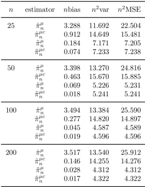
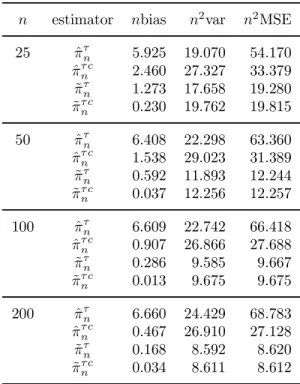
The simulation results are largely consistent with the theory derived in the paper. The bias of ^¼n is quite noticeable and does not vanish as the sample size increases. It turns out, however, that the bootstrap is quite e®ective in reducing the bias of ^¼n. The bootstrap reduces the bias of ^¼nsubstantially in all cases that we consider in our simulations, and the bias reduction becomes more e®ective as the sample size increases. In some of the reported cases, the bias corrected estimate has bias as small as approximately 2% of that of ^¼n. On the other hand, the bootstrap bias correction has little impact on the sampling variation.

The sample variances of ^¼cn are roughly comparable to, or even slightly larger than, those of ^¼n. The bootstrap also reduces the bias in ~¼n, albeit the magnitudes of improvements are not comparable to those for ^¼n. Clearly, ~¼n is asymptotically unbiased, and thus there is not as much room for improvement in ~¼n as in ^¼n. The bootstrap does not reduce the sampling variations for ~¼n, just as for ^¼n, and ~¼c_nhas no smaller sample variances. For both estimators, the bootstrap bias corrections become relatively more important for models with a mean or a linear trend.

It appears that the bootstrap generates quite precise critical values for both tests ^Tn and ~Tn, even when the sample sizes are small. In particular, the performance of ^T¤

n is quite satisfactory. The test ^Tn is invalid, and naturally, yields the rejection probabilities under the null that are very distinct from its nominal test sizes. However, its bootstrap version ^T_n¤ has quite accurate null rejection probabilities even for small samples. As expected, the test

~

Tnbased on the e±cient estimator ~¼nperforms much better than its OLS counterpart ^Tnin terms of the rejection probabilities under the null. Its bootstrap version ~T_n¤also improves the ¯nite sample performances of ~Tn. While the null rejection probabilities of both bootstrap tests ^Tn¤and ~Tn¤approach to the nominal values as the size of samples increase, the bootstrap e±cient test ~T_n¤ does better in small samples than its OLS counterpart ^T_n¤. This is more so for models with a mean or a linear trend. Due to the presence of non-uniform size distortions, the ¯nite sample power comparisons between ^Tn and ~Tn and their bootstrap counterparts ^T_n¤ and ~T_n¤ are not clear. It just seems that they are all roughly comparable.

5. Conclusion

In this paper we consider the bootstrap for cointegrating regressions. We introduce the sieve bootstrap based on a VAR of order increasing with the sample size, and establish its consistency and asymptotic validity for two procedures: the usual OLS and the e±cient OLS relying on the regressions augmented with the leads and lags of the di®erenced re-gressors. For the usual OLS, the bootstrap can thus be employed to correct for biases in the estimated parameters, and to compute the critical values of the tests. With the boot-strap bias correction, the OLS estimator becomes asymptotically unbiased. Moreover, the OLS-based tests become asymptotically valid, if the bootstrap critical values are used. The bootstrap OLS method, however, is not e±cient. For the e±cient inference, we should base our bootstrap procedure on the e±cient OLS method. The sieve bootstrap proposed in the paper appears to improve upon the e±cient OLS method in ¯nite samples. It generally reduces the ¯nite sample biases for the estimators and yields sizes that are closer to the nominal sizes of the tests.

The theory and method developed in the paper can be used to analyze more general cointegrated models. The models with deterministic trends and/or structural breaks can be analyzed similarly. The error correction models, seemingly unrelated and panel cointe-gration models are other examples, to which our theory and method are readily applicable. Indeed, the required modi¯cations of the theory and method for such extensions are mini-mal, and can be applied only with some obvious adjustments. The theory discussed in the paper is concerned only with the consistency of the bootstrap. For the pivotal statistics,

however, it might well be the case that the bootstrap provides the asymptotic re¯nements as well. Our simulation study in the paper is in fact somewhat indicative of this possibility. Moreover, it appears that the theoretical illustration for the asymptotic re¯nement is pos-sible using the techniques developed in Park (2000) to establish the bootstrap re¯nement for the unit root tests.

6. Mathematical Proofs

6.1 Useful Lemmas and Their Proofs

We consider the regression

wt= ~©1wt¡1+¢ ¢ ¢+ ~©qwt¡q+ ~"qt (23) which is the ¯tted version of regression (15). Since ¦n is consistent, it is well expected that the ¯tted regression (23) with (wt) should be asymptotically equivalent to the ¯tted regression (16) with ( ^wt) introduced in Step 1 of our bootstrap procedure.

Lemma A1 Under Assumptions 2.1 and 3.1, we have asn! 1

^ ©k= ~©k+Op(n¡1=2) uniformly in 1·k·q. Moreover, max 1·t·nj^"qt¡~"qtj=Op(n ¡1=2₎ as n! 1.

Proof of Lemma A1 It follows immediately from the de¯nition of ( ^wt) that max 0·i;j·q ¯ ¯¯ ¯ ¯ 1 n n X t=1 ^ wt¡iw^t0¡j¡ 1 n n X t=1 wt¡iw0t¡j ¯ ¯¯ ¯ ¯· µ max 1·t·njwt^ ¡wtj ¶ Ã₁ n n X t=1 jwt^ j+ 1 n n X t=1 jwtj ! However, we have max 1·t·njwt^ ¡wtj=Op(n ¡1=2₎ because jwt^ ¡wtj= ¯ ¯¯ ¯ ¯ à yt¡¦0nxt vt ! ¡wt ¯ ¯¯ ¯ ¯= ¯ ¯¯ ¯ ¯ à (¦¡¦n)0xt 0 !¯¯_¯ ¯ ¯· j¦¡¦nj jxtj and j¦n¡¦j=Op(n¡1); max 1·t·njxtj=Op(n 1=2₎ Since 1 n n X t=1 jwtj; 1 n n X t=1 jwt^j=Op(1)

we have max 0·i;j·q ¯ ¯ ¯ ¯ ¯ 1 n n X t=1 ^ wt¡iw^t0¡j¡ 1 n n X t=1 wt¡iw0t¡j ¯ ¯ ¯ ¯ ¯=Op(n 1=2₎ The rest of the proof is rather straightforward, and we omit the details.

Let

w·t= (w0_t¡1; : : : ; w_t0_¡·)0 and de¯ne

M··=Ew·tw_·t0

Moreover, denote byf the spectral density of (wt). Then we have Lemma A2 Under Assumption 2.1, we have

° °°M_··¡1°°°· _2¼1 µ inf ¸ kf(¸)k ¶_¡1 for all·¸1.

Proof of Lemma A2 Let c·2R· be an eigenvector associated with the smallest eigen-value¸min of M··. De¯ne

'·(¸) = (ei¸; : : : ; ei·¸)0 and use \¹" to denote its cojugate. It follows that

¸min = c0·M··c· = Z ¼ ¡¼c 0 · ¡ '·(¸)¹'·(¸)0-f(¸) ¢ c·d¸ ¸ Z ¼ ¡¼ µ inf ¸ °°'·(¸)¹'·(¸) 0_-f(¸)°°¶_d¸ = µ inf ¸ kf(¸)k ¶ Z ¼ ¡¼k'·(¸)¹'·(¸) 0_kd¸ = 2¼ µ inf ¸ kf(¸)k ¶ However, we have _° ° °M_··¡1°°°=¸¡_min1 from which the stated result can be deduced immediately. Lemma A3 Under Assumptions 2.1 and 3.1, we have

sup ¸ jf ¤_{(¸)¡f(¸)j=o}¤ p(1) and 1 X k=¡1 ¡¤(k) = 1 X k=¡1 ¡(k) +o¤_p(1) as n! 1.

Proof of Lemma A3 Given Lemma A1, the stated results are just straightforward ex-tensions of Lemma A2 in Chang and Park (2002b). Here we only obtain `in probability' versions, instead of `almost sure' versions, since the results in Lemma A1 hold only in probability.

Lemmma A4 Under Assumptions 2.1and 3.1, we have

E¤¯¯¯¯_¯ n X t=1 (wt¤¡iw¤0t¡j¡¡¤(i¡j)) ¯¯ ¯ ¯ ¯ 2 =Op(n) uniformly in iand j, asn! 1.

Proof of Lemma A4 Once again, the stated result follows exactly as in Lemma A4 in Chang and Park (2002b), due to Lemma A1, under some obvious modi¯cations to deal with multiple time series.

Lemmma A5 Under Assumptions 2.1, 2.3and 3.1, we have

E¤ °° ° ° ° ° à 1 n n X t=1 vpt¤vpt¤0 !¡1°° ° ° ° ° = Op(1) E¤ ¯ ¯¯ ¯ ¯ n X t=1 x¤tv¤0pt ¯ ¯¯ ¯ ¯ = Op(np 1=2₎ as n! 1.

Proof of Lemma A5 The proof is essentially identical to that of Lemma 3.3 in Chang and Park (2002b).

Lemma A6 Under Assumptions 2.1, 2.3and 3.1,we have

¯ ¯¯ ¯ ¯ n X t=1 v_pt¤´¤0_pt ¯ ¯¯ ¯ ¯=Op¤(n1=2p1=2) and _n X t=1 x¤t(´¤t ¡´¤pt)0 =o¤p(n) as n! 1.

Proof of Lemma A6 De¯ne ( ^ªpk) such that ´¤_pt¡´¤_t = X jkj>p ^ ¦0_kv¤_t¡k= X jkj>p ^ ªpk"¤_t¡k

Note that X jkj>p jªpk^ j · Ã ₁ X k=1 jªk^ j ! 0 @X jkj>p j¦k^ j 1 A

as one may easily deduce.

To show the ¯rst part, we write for 1·i·p n X t=1 vt¤¡i´¤0pt = n X t=1 vt¤¡i´¤0t + n X t=1 vt¤¡i(´¤pt¡´¤t)0 It is easy to see E¤ ¯ ¯¯ ¯ ¯ n X t=1 vt¤¡i´¤0t ¯ ¯¯ ¯ ¯ 2 =Op(n) uniformly in 1·i·p. Therefore, it su±ces to show that

n

X

t=1

vt¤¡i(´¤pt¡´¤t)0=o¤p(n1=2) (24)

uniformly in 1·i·p. However, we have as in the proof of Lemma 3.1 in Chang and Park (2002a) n X t=1 w¤t¡i 0 @X jjj>p ^ ªpj"¤t¡j 1 A 0 = 0 @X jkj>p jªk^ ¡1jjªpk^ j 1 AOp¤(n) + 0 @X1 i=0 X jjj>p jªi^ jjªpj^ j 1 AOp¤(n1=2) = 0 @X jkj>p jªpk^ j 1 AOp¤(n1=2) = 0 @X jkj>p j¦k^ j 1 AO_p¤(n1=2)

uniformly in 1·i·p, and (24) follows immediately. To prove the second part, we de¯ne

xi¤t = t X i=1 "¤i (25) so that zt¤= ^ª(1)»¤t + ( ¹w0¤¡w¹¤t) It follows that n X t=1 zt¤(´¤pt¡´¤t)0= ^ª(1) n X t=1 »¤t(´¤pt¡´¤t)0+ ¹w0¤ n X t=1 (´¤pt¡´¤t)0¡ n X t=1 ¹ wt¤(´¤pt¡´¤t)0 (26)

We have n X t=1 (´¤_pt¡´¤_t) = X jkj>p ^ ªpk n X t=1 "¤_t¡k = 0 @X jkj>p jªpk^ j 1 AO¤_p(n1=2) = 0 @X jkj>p j¦k^ j 1 AO¤_p(n1=2) (27)

We also have similarly as in the proof of the ¯rst part n X t=1 ¹ w¤_t(´¤_pt¡´¤_t)0= 0 @X jkj>p j¦k^ j 1 AO¤_p(n) (28) Moreover, we have as in the proof of Lemma 3.1 in Chang and Park (2002a)

n X t=1 »¤t(´¤pt¡´¤t)0 = 0 @X jkj>p jªpk^ j 1 AO¤p(n) + 0 @X jkj>p jªpk^ j 1 AO¤p(n1=2) = 0 @X jkj>p j¦k^ j 1 AO¤p(n) (29)

The second part can now be easily deduced from (26) and (27) - (29). The proof is therefore complete.

6.2 Proofs of Lemmas and Theorems

Proof of Lemma 2.2 The stated result follows from Einmahl (1987). In particular, he shows that his Equation 1.3 holds for all ± when 2 < s < 4, and for ± ¸ K°

sn with ° <1=(2s¡4) when s¸4, in his notation. In either case, his± is greater than ourn1=a+± with any ± > 0 as long as n is su±ciently large. His result is therefore applicable as we formulate here.

Proof of Lemma 2.4 We write n( ~¦n¡¦) = à 1 n2 n X t=1 xtx0t¡Qn !¡1à 1 n n X t=1 xt´t¡Pn ! where Pn = 1 n n X t=1 xt(´_t¡´_pt)0+ à 1 n n X t=1 xtv0_pt ! à 1 n n X t=1 vptv0_pt !¡1à 1 n n X t=1 vpt´0_pt ! Qn = 1 n à 1 n n X t=1 xtv_pt0 ! à 1 n n X t=1 vptv_pt0 !¡1à 1 n n X t=1 vptx0_t !

where in turn

vpt= (v0_t+p; : : : ; v0_t¡p)0 To get the stated result, it su±ces to show that

Pn; Qn=op(1) under Assumptions 2.1 and 2.3.

In the subsequent proof, we use

° ° ° ° ° 1 n n X t=1 xtvpt0 ° ° ° ° ° = Op(p 1=2_{) (30)} °° ° ° ° ° Ã 1 n n X t=1 vptv_pt0 !_¡1°° ° ° ° ° = Op(1) (31)

which are the multivariate extensions of the results established in Chang and Park (2002a). The required extensions are straightforward and the details are omitted. It follows imme-diately from (30) and (31) that

Qn=n¡1Op(p1=2)Op(1)Op(p1=2) =Op(n¡1p) since kQnk · _n1 ° °° ° ° 1 n n X t=1 xtv0pt ° °° ° ° ° °° ° ° ° Ã 1 n n X t=1 vptv0pt !¡1°_°° ° ° ° ° °° ° ° 1 n n X t=1 vptx0t ° °° ° °

as one may easily see. We now show that

Pn= 0 @X jkj>p j¦kj 1 AOp(1) +Op(n¡1=2p) We ¯rst write kPnk · ° ° ° ° ° 1 n n X t=1 xt(´pt¡´t)0 ° ° ° ° °+ ° ° ° ° ° 1 n n X t=1 xtvpt0 ° ° ° ° ° ° ° ° ° °° Ã 1 n n X t=1 vptvpt0 !¡1°° ° ° °° ° ° ° ° ° 1 n n X t=1 vpt´0pt ° ° ° ° ° = An+Bn

We may show as in the proof of Lemma 3.1 of Chang and Park (2002a) that An= 0 @X jkj>p j¦kj 1 AOp(1)

Moreover, we have ¯ ¯¯ ¯ ¯ n X t=1 vt¡i´0pt ¯ ¯¯ ¯ ¯ · ¯ ¯¯ ¯ ¯ ¯ n X t=1 vt¡i 0 @ut¡ X jjj·p ¦0kvt¡j 1 A 0¯ ¯¯ ¯ ¯ ¯ · ¯ ¯ ¯ ¯ ¯ n X t=1 vt_¡iu0_t ¯ ¯ ¯ ¯ ¯+ 1 X j=¡1 j¦jj ¯ ¯ ¯ ¯ ¯ n X t=1 vt_¡iv0_t¡j ¯ ¯ ¯ ¯ ¯ = Op(n1=2) uniformly in iforjij ·p. It therefore follows that

Bn=Op(p1=2)Op(1)Op(n¡1=2p1=2) =Op(n¡1=2p) as was to be shown.

Proof of Lemma 3.2 Given the result in Lemma A1, the proof is the trivial extension of the proof of Lemma 3.2 in Park (2002). The details are, therefore, omitted.

Proof of Theorem 3.3 To derive the bootstrap invariance principle for (wt¤) from that of ("¤ t), we need to show ^ ©(1)!p©(1) (32) and P¤ ½ max 1·t·n ¯ ¯¯n¡1=2w¹¤_t¯¯¯> ² ¾ =op(1) (33) for any² >0.

Let ~©(1) be de¯ned exactly as ^©(1) using the ¯tted coe±cients ( ~©k) in regression (23). It follows immediately from Lemma A1 that

^

©(1) = ~©(1) +Op(n¡1=2q)

Moreover, we may deduce as in the proof of Lemma 3.5 in Chang and Park (2002a) that ~

©(1) = ©(1) +Op(n¡1=2q) +o(q¡b) using the result in Shibata (1981). We therefore have

^

©(1) = ©(1) +op(1)

and obtain (32). The proof of (33) is essentially identical to the proof of Theorem 3.3 in Park (2002).

Proof of Lemma 3.4 Setz0¤ = 0 for simplicity. The required modi¯cation to allow for nonzeroz¤₀ is trivial. The ¯rst part follows immediately, since

1 n2 n X t=1 zt¤z¤0t =d¤ Z 1 0 B ¤ nBn¤0+ 1 n2zn¤zn¤0 and n¡1=2zn¤ =O¤p(1) for largen.

To prove the second part, we let (»¤_t) be de¯ned as in (25) so that we have n X t=1 zt¤¡1wt¤0 = ª(1)^ n X t=1 »¤t¡1"¤0tª(1)^ 0+ n X t=1 wt¤w¹t¤0 ¡z¤nw¹¤0n + ¹w¤0 n X t=1 "¤0tª(1)^ 0¡ n X t=1 ¹ wt¤¡1"¤0t ª(1)^ 0 It is straightforward to show z_n¤w¹¤0_n; w¹₀¤ n X t=1 "¤0_t ª(1)^ 0; n X t=1 ¹ w_t¤_¡1"¤0_tª(1)^ 0=O_p¤(n1=2)

and we therefore have n X t=1 z¤_t¡1w¤0_t = ^ª(1) n X t=1 »¤_t¡1"¤0_tª(1)^ 0+ n X t=1 w¤_tw¹_t¤0+o¤_p(1) (34) for largen. It follows that ^ ª(1) n X t=1 »¤_t¡1"¤0_t ª(1)^ 0 !d¤ Z 1 0 BdB 0

by the bootstrap invariance principle and Kurtz and Protter (1991). Moreover, it can be deduced analogously as in Lemma A4 that

E¤ ¯ ¯ ¯ ¯¯ n X t=1 (w¤tw¹¤0t ¡E¤wt¤w¹t¤0) ¯ ¯ ¯ ¯¯ 2 =Op(n2) and we have 1 n n X t=1 wt¤w¹t¤0=E¤wt¤w¹¤0t +Op¤(n¡1=2) However, E¤wt¤w¹¤0t = 1 X k=0 ¡¤(k) = 1 X k=0 ¡(k) +o¤p(1) from which, together with (34), the stated result follows immediately.

Proof of Theorem 3.5 The results can easily be derived from Lemma 3.4 using the bootstrap invariance principle and continuous mapping theorem.

Proof of Lemma 3.6 Notice that

jQ¤_nj · 1 n ¯¯ ¯ ¯ ¯ 1 n n X t=1 x¤_tv¤0_pt¯¯¯_¯ ¯ °° ° ° ° ° à 1 n n X t=1 v¤_ptv_pt¤0 !_¡1°° ° ° ° ° ¯¯ ¯ ¯ ¯ 1 n n X t=1 vptx¤0_t ¯¯¯_¯ ¯

It therefore follows that

Q¤_n=n¡1O_p¤(p1=2)O_p¤(1)O_p¤(p1=2) =O¤_p(n¡1p) from Lemma A5. This shows thatQ¤n=o¤p(1).

Moreover, we have jP_n¤j · ¯ ¯¯ ¯ ¯ 1 n n X t=1 x¤_t(´¤_pt¡´¤_t)0 ¯ ¯¯ ¯ ¯+ ¯ ¯¯ ¯ ¯ 1 n n X t=1 x¤_tv¤0_pt ¯ ¯¯ ¯ ¯ ° ° °° ° ° à 1 n n X t=1 v¤_ptv¤0_pt !_¡1°° °° ° ° ¯ ¯¯ ¯ ¯ 1 n n X t=1 vpt´¤0_pt ¯ ¯¯ ¯ ¯

and it follows from Lemmas A5 and A6 that

Pn=o¤_p(1) +O¤_p(p1=2)O¤_p(1)O¤_p(n¡1=2p1=2) =o¤_p(1) as required to be shown.

Proof of Theorem 3.7 Due to Lemma 3.6, we have n( ~¦¤n¡¦n) = à 1 n2 n X t=1 x¤tx¤0t !¡1 1 n n X t=1 x¤t´¤0t +o¤p(1) The bootstrap asymptotic distribution of ~¦¤

ncan now be easily deduced from the bootstrap invariance principle and Kurtz and Protter (1991). The bootstrap asymptotic distribution of ~Tn¤ may similarly be obtained.

References

Basawa, I.V., A.K. Mallik, W.P. McCormick, J.H. Reeves and R.L. Taylor (1991a). \Boot-strapping unstable ¯rst-order autoregressive processes,"Annals of Statistics19: 1098-1101.

Chang, Y. and J.Y. Park (2002a). \On the asymptotics of ADF tests for unit roots," forthcoming inEconometric Reviews.

Chang, Y. and J.Y. Park (2002b). \A sieve bootstrap for the test of a unit root," forth-coming inJournal of Time Series Analysis.

Einmahl, U. (1987). \A useful estimate in the multidimensional invariance principle,"

Probability Theory and Related Fields 76: 81-101.

Horowitz, J. (2002). \The bootstrap," forthcoming in Handbook of Econometrics Vol. 5, Elsevier, Amsterdam.

Johansen, S. (1988). \Statistical analysis of cointegration vectors," Journal of Economic Dynamics and Control 12: 231-254.

Johansen, S. (1991). \Estimation and hypothesis testing of cointegration vectors in Gaus-sian vector autoregressive models,"Econometrica 59: 1551-1580.

Kurtz, T.G. and P. Protter (1991). \Weak limit theorems for stochastic integrals and stochastic di®erential equations,"Annals of Probability 19: 1035-1070.

Li, H. and J.S. Maddala (1997). \Bootstrapping cointegrating regressions," Journal of Econometrics 80: 297-348.

Park, J.Y. (2000). \Bootstrap unit root tests," Mimeographed, School of Economics, Seoul National University.

Park, J.Y. (2002). \An invariance principle for sieve bootstrap in time series," forthcoming inEconometric Theory.

Park, J.Y. and P.C.B. Phillips (1988). \Statistical inference in regressions with integrated processes: Part 1,"Econometric Theory4: 468-497.

Phillips, P.C.B. and V. Solo (1992). \Asymptotics for linear processes,"Annals of Statistics

20: 971-1001.

Saikkonen, P. (1991). \Asymptotically e±cient estimation of cointegration regressions,"

Econometric Theory 7: 1-21.

Shibata, R. (1980). \Asymptotically e±cient selection of the order of the model for esti-mating parameters of a linear process," Annals of Statistics 8: 147-164.

Stock, J.H. and M.W. Watson (1993). \A simple estimator of cointegrating vectors in higher order integrated systems,"Econometrica 61: 783-820.

Table 1.1: Finite Sample Performances of the Estimators

n estimator nbias n2_{var n}2_MSE

25 ¼^n 2.516 4.826 11.157 ^ ¼c_n 0.576 6.315 6.647 ~ ¼n 0.025 2.981 2.982 ~ ¼c_n 0.026 2.981 2.981 50 ¼^n 2.705 6.213 13.528 ^ ¼c_n 0.365 7.305 7.439 ~ ¼n 0.015 2.489 2.489 ~ ¼c n 0.016 2.490 2.490 100 ¼^n 2.746 6.573 14.112 ^ ¼c_n 0.197 7.201 7.240 ~ ¼n 0.015 2.224 2.224 ~ ¼c_n 0.014 2.229 2.229 200 ¼^n 2.723 6.457 13.871 ^ ¼c_n 0.060 6.775 6.779 ~ ¼n -0.005 2.165 2.165 ~ ¼c_n -0.004 2.169 2.169

Table 1.2: Finite Sample Performances of the Test Statistics

sizes powers

n test 1% test 5% test 10% test 1% test 5% test 10% test

25 T^n 0.058 0.216 0.345 0.583 0.806 0.885 ^ T¤ n 0.011 0.053 0.100 0.404 0.558 0.660 ~ Tn 0.046 0.110 0.178 0.485 0.626 0.691 ~ T_n¤ 0.007 0.045 0.090 0.296 0.481 0.592 50 T^n 0.055 0.195 0.324 0.893 0.977 0.990 ^ T¤ n 0.008 0.048 0.097 0.727 0.873 0.934 ~ Tn 0.026 0.080 0.131 0.811 0.892 0.919 ~ T¤ n 0.012 0.051 0.097 0.744 0.856 0.902 100 T^n 0.047 0.174 0.296 0.997 1.000 1.000 ^ T_n¤ 0.010 0.047 0.094 0.981 0.997 0.999 ~ Tn 0.018 0.066 0.117 0.982 0.994 0.997 ~ T_n¤ 0.010 0.049 0.096 0.973 0.991 0.996 200 T^n 0.039 0.161 0.270 1.000 1.000 1.000 ^ T¤ n 0.009 0.045 0.094 1.000 1.000 1.000 ~ Tn 0.012 0.054 0.105 1.000 1.000 1.000 ~ Tn¤ 0.009 0.045 0.096 1.000 1.000 1.000

Table 2.1: Finite Sample Performances of the Estimators

n estimator nbias n2_{var n}2_MSE 25 ^¼¹_n 3.288 11.692 22.504 ^ ¼¹c_n 0.912 14.649 15.481 ~ ¼¹_n 0.184 7.171 7.205 ~ ¼¹c_n 0.074 7.233 7.238 50 ^¼¹_n 3.398 13.270 24.816 ^ ¼¹c_n 0.463 15.670 15.885 ~ ¼¹_n 0.069 5.226 5.231 ~ ¼¹c_n 0.018 5.241 5.241 100 ^¼¹_n 3.494 13.384 25.590 ^ ¼¹c_n 0.277 14.820 14.897 ~ ¼¹_n 0.045 4.587 4.589 ~ ¼¹c_n 0.019 4.596 4.596 200 ^¼¹_n 3.517 13.540 25.912 ^ ¼¹c_n 0.146 14.255 14.276 ~ ¼¹_n 0.028 4.312 4.312 ~ ¼¹c_n 0.017 4.322 4.322

Table 2.2: Finite Sample Performances of the Test Statistics

sizes powers

n test 1% test 5% test 10% test 1% test 5% test 10% test 25 T^¹ n 0.020 0.142 0.261 0.265 0.547 0.676 ^ T¹¤ n 0.017 0.059 0.106 0.227 0.384 0.498 ~ T_n¹ 0.044 0.117 0.180 0.257 0.415 0.505 ~ T¹¤ n 0.008 0.043 0.090 0.093 0.248 0.369 50 T^_n¹ 0.031 0.140 0.257 0.623 0.841 0.905 ^ T¹¤ n 0.011 0.055 0.106 0.498 0.693 0.795 ~ T¹ n 0.026 0.084 0.135 0.591 0.736 0.808 ~ T¹¤ n 0.012 0.052 0.102 0.479 0.672 0.767 100 T^¹ n 0.029 0.135 0.231 0.967 0.994 0.997 ^ T¹¤ n 0.010 0.054 0.105 0.924 0.978 0.990 ~ T¹ n 0.017 0.067 0.121 0.942 0.974 0.984 ~ T¹¤ n 0.011 0.051 0.099 0.921 0.967 0.980 200 T^¹ n 0.026 0.125 0.220 1.000 1.000 1.000 ^ T¹¤ n 0.011 0.052 0.100 1.000 1.000 1.000 ~ T¹ n 0.014 0.060 0.115 0.999 1.000 1.000 ~ Tn¹¤ 0.010 0.050 0.103 0.999 1.000 1.000

Table 3.1: Finite Sample Performances of the Estimators

n estimator nbias n2_{var n}2_MSE 25 ^¼¿_n 5.925 19.070 54.170 ^ ¼¿ c_n 2.460 27.327 33.379 ~ ¼¿_n 1.273 17.658 19.280 ~ ¼¿ c_n 0.230 19.762 19.815 50 ^¼¿_n 6.408 22.298 63.360 ^ ¼¿ c_n 1.538 29.023 31.389 ~ ¼¿_n 0.592 11.893 12.244 ~ ¼¿ c_n 0.037 12.256 12.257 100 ^¼¿_n 6.609 22.742 66.418 ^ ¼¿ c_n 0.907 26.866 27.688 ~ ¼¿_n 0.286 9.585 9.667 ~ ¼¿ c_n 0.013 9.675 9.675 200 ^¼¿_n 6.660 24.429 68.783 ^ ¼¿ c_n 0.467 26.910 27.128 ~ ¼¿_n 0.168 8.592 8.620 ~ ¼¿ c_n 0.034 8.611 8.612

Table 3.2: Finite Sample Performances of the Test Statistics

sizes powers

n test 1% test 5% test 10% test 1% test 5% test 10% test 25 T^¿ n 0.051 0.212 0.351 0.204 0.503 0.661 ^ T¿¤ n 0.029 0.071 0.123 0.120 0.243 0.355 ~ T_n¿ 0.056 0.135 0.203 0.161 0.298 0.388 ~ T¿¤ n 0.010 0.042 0.091 0.035 0.131 0.228 50 T^_n¿ 0.060 0.246 0.387 0.522 0.790 0.879 ^ T¿¤ n 0.016 0.057 0.114 0.271 0.490 0.612 ~ T¿ n 0.025 0.080 0.134 0.329 0.516 0.612 ~ T¿¤ n 0.010 0.050 0.100 0.221 0.430 0.551 100 T^¿ n 0.065 0.235 0.375 0.927 0.987 0.995 ^ T¿¤ n 0.010 0.056 0.108 0.753 0.905 0.951 ~ T¿ n 0.015 0.064 0.116 0.815 0.904 0.938 ~ T¿¤ n 0.009 0.049 0.099 0.770 0.886 0.927 200 T^¿ n 0.062 0.229 0.362 1.000 1.000 1.000 ^ T¿¤ n 0.012 0.056 0.107 0.998 1.000 1.000 ~ T¿ n 0.014 0.057 0.109 0.997 0.999 0.999 ~ Tn¿¤ 0.011 0.050 0.101 0.996 0.999 0.999