Experimental study of cognitive radio test-bed using USRP

(1)

Louisiana State University

LSU Digital Commons

LSU Master's Theses Graduate School

2011

Experimental study of cognitive radio test-bed

using USRP

Venkat vinod Patcha

Louisiana State University and Agricultural and Mechanical College, [email protected]

Follow this and additional works at:https://digitalcommons.lsu.edu/gradschool_theses

Part of theElectrical and Computer Engineering Commons

This Thesis is brought to you for free and open access by the Graduate School at LSU Digital Commons. It has been accepted for inclusion in LSU Master's Theses by an authorized graduate school editor of LSU Digital Commons. For more information, please [email protected].

Recommended Citation

Patcha, Venkat vinod, "Experimental study of cognitive radio test-bed using USRP" (2011).LSU Master's Theses. 481.

(2)

EXPERIMENTAL STUDY OF COGNITIVE RADIO TEST-BED USING USRP

Thesis

Submitted to the Faculty of the Louisiana State University and Agricultural and Mechanical College

in partial fulfillment of the requirements for the degree of Master of Science in Electrical Engineering

in

The Department of Electrical and Computer Engineering

by

Venkat vinod Patcha

B.TECH in Electronics and Communication Engineering

Padmasri Dr. B.V. Raju Institute of Technology (Affiliated to JNTU), India, 2008. August, 2011

(3)

Acknowledgments

First of all, I would like to express sincere gratitude to my adviser Dr. Shuangqing Wei for his constant support in building my thesis. I would like to thank him for introducing me to the field of Wireless Communication and Cognitive Radio. His throughout guidance and motivation in solving complex problems has provided encouragement, enthusiasm and sup-port, while the knowledge acquired by working with him has provided deep understanding of issues that are apart from classroom work. Also, I would like to thank my Co-adviser Dr. Rajgopal Kannan, whose support has provided valuable experience. I would thank Dr. Xue-bin Liang for being a member of thesis committee.

Apart from all, my parents and elder sister have provided the emotional and financial support to build my confidence and without which this wouldn’t be possible. I would like to thank my friends and roommates for their support and morale boost during the hard times. Also, I would like to mention my lab-mates for giving their resources and time in enabling to complete my thesis.

(4)

List of Tables

5.1 Performance of PU: short burst of traffic from SU . . . 49

5.2 Performance of PU: long burst of traffic from SU . . . 49

5.3 Performance of SU: short burst of traffic from SU . . . 50

5.4 Performance of SU: long burst of traffic from SU . . . 50

5.5 Performance of PU:long burst of traffic from PU and SU . . . 51

5.6 Performance of SU: long burst of traffic from PU and SU . . . 51

5.7 Performance of PU for two-channel without hand-sake . . . 55

5.8 Performance of SU for two-channel without hand-sake . . . 55

5.9 Performance of PU for two-channel with two-way handshake . . . 59

5.10 Performance of SU for two-channel with two-way handshake . . . 59

5.11 Performance of PU for two-channel with three-way handshake(DBPSK) . . 63

5.12 Performance of SU for two-channel with three-way handshake(DBPSK) . . 63

5.13 Performance of PU for two-channel with three-way handshake(GMSK) . . 64

5.14 Performance of SU for two-channel with three-way handshake(GMSK) . . . 64

(8)

List of Figures

1.1 Frequency Usage of Spectrum Bands [9] . . . 2

1.2 Hardware (USRP version 1) and Architecture [4] . . . 4

2.1 2-D Illustration of Piece-wise Periodogram Analysis . . . 10

2.2 Block Diagram for Piece-Wise Periodogram Analysis . . . 11

2.3 Block Diagram for sensing model . . . 12

2.4 PSD and Curve-fitting plot under H0 . . . 13

2.5 PSD and Curve-fitting plot under H1 . . . 13

2.6 Histogram and density plots of average channel power for H0andH1 . . . 14

2.7 Histogram and density plots of average channel power for different time windows underH1 . . . 15

2.8 Histogram and density plots of average channel power for different window-ing functions underH1 . . . 16

3.1 Block Diagram for two state Markov model . . . 18

3.2 Block Diagram for DBPSK modulation . . . 19

3.3 MATLAB plot for PSD of DBPSK modulated waveform using equation (3.5) 21 3.4 PSD of DBPSK modulated waveform on Spectrum Analyzer . . . 21

4.1 Flow-graph for OFDM model [12] . . . 24

4.2 Training Sequence for Symbol Synchronization [12] . . . 25

(9)

4.4 Approach 1: Flow-graph for coded OFDM transmitter . . . 32

4.5 Approach 1: Flow-graph for coded OFDM receiver . . . 32

4.6 Approach 2: Flow-graph for coded OFDM receiver . . . 33

4.7 Working Model: Flow-graph for coded OFDM receiver . . . 35

4.8 Packet structure for coded OFDM model . . . 36

4.9 Packet flow for coded OFDM model . . . 37

4.10 Modified Header Packet Structure . . . 39

5.1 Block Diagram for sensing-transmission flow graphs . . . 43

5.2 Time Division Multiplexing of sensing-transmission periods . . . 44

5.3 Block Diagram for sensing, reception and transmission flow graphs . . . 44

5.4 Time Division Multiplexing of sensing-reception-sensing-transmission periods 45 5.5 Test-bed Model for PU’s and SU’s . . . 46

5.6 Duty cycle of SU’s for two channel and without mutual handshake . . . 53

5.7 Flow Chart for two-way handshake . . . 57

5.8 Duty cycle of SU’s for two channel and with two-way handshake . . . 58

5.9 Flow Chart for three-way handshake . . . 61

5.10 Duty cycle of SU’s for two channel and with three-way handshake . . . 62

5.11 Multimedia Traffic for Primary Users . . . 66

(10)

Abstract

Cognitive Radio is an emerging technology that enables efficient utilization of the spectrum. As such, it has created great interests in industrial and research fields. Many people have proposed test-bed models for the performance analysis of primary and secondary users in a real-time noise environment. However, these test-beds are generally lacking in their range of capabilities as well as accurate implementation of the proposed models. In this thesis, we develop our test-bed on USRP to achieve the spectrum sensing and co-existence of primary and secondary users, while implementing the rendezvous protocols for secondary traffic coordination.

We first demonstrate the spectrum sensing on the primary users using an energy detec-tor(Average periodogram analysis) to obtain the average power of the primary channel under two different channel conditions (busy or idle). The focus is extended on developing the Markov traffic model and the Coded OFDM transceivers, while discussing the practical limitations for Markov traffic and viable solutions for reducing the burst errors for Coded OFDM . Finally, a four-node test-bed model of primary and secondary users is analyzed with the interference metrics(packet loss and error rate) for different scenario’s. Also, the throughput and the interference metrics are compared for different rendezvous protocols of the secondary users.

(11)

Chapter 1 Introduction

Wireless Communication has been a rapidly growing sector in the communication industry that led to rise of market share and economic growth. In fact, the growth of wireless communication has created new technologies, which provide services with high bandwidth. From the beginning of the 20th century, there has been an increase in the usage of radio spectrum in areas such as Mobile communication, Wireless Local Area Network (WLAN), Blue-tooth and Cordless phones. The Federal Communication Commission (FCC), which manages the radio frequency spectrum and its usage, has published a report on the precise usage of the spectrum and the rise of unlicensed users that could cause interference to the licensed users [5]. In addition, the report has stressed on frequency bands that are heavily occupied all the time or partially occupied or vacant most of the time [5]. The Figure 1.1 signifies the usage of spectrum bands over a certain period. The scarcity of spectrum and need for efficient usage has led to the development of a new field ”Cognitive Radio”. The term was first coined by Joseph Mitola in his thesis that emphasizes the efficient usage of spectrum and its allocation [9]. Cognitive Radio (CR) is a type of radio, that is aware of its environment, in which the radio adapts its transmission for efficient usage of the underutilized spectrum. The central idea of CR is to allow the unlicensed bands of the Secondary Users(SU), such as WLAN and Blue-tooth to utilize the licensed bands of the Primary Users(PU), such as TV and mobile without interference. The main features of cognitive radio are intelligence, adaptivity, reliability and efficiency [8]. It is a key contribution to the 4th generation (4G) technology for the efficient spectrum utilization [9]. The practical implementation of CR has been achieved by Software Defined Radio (SDR). SDR is a radio communication system in which the components implemented on hardware are transferred to a software program that provides the flexibility of changing the operating parameters of the device. The primary advantage of SDR is to use them over wide RF bandwidth and to perform Intermediate frequency(IF) functions inside the processor. In fact, Cognitive Radio is defined as ”intelligence” that sits above SDR and lets SDR determine which mode of operation and parameter to use [19]. As SDR handsets can

(12)

Figure 1.1: Frequency Usage of Spectrum Bands [9]

easily be re-configured to different wireless broadband technologies, they can be utilized to implement a CR Test-bed. The flexibility, robustness and efficiency of SDR has resulted in practical experimentation over RF world.

1.1 Motivation

Many features of Cognitive Radio have attracted researchers, while studies are conducted for efficient utilization. The flexibility and growth of SDR has provided ease of implemen-tation of a Cognitive Radio test-bed. They provide the ease of implemenimplemen-tation by using software to build a network and to modify the network based on the availability. The major contribution in our thesis is to create a test-bed model for evaluating the spectrum access and co-existence of primary and secondary users and study their performance analysis, while emphasizing the usage of existing rendezvous protocols for secondary users(SU) to reduce interference effects and provide high throughput.

1.2 Contribution of Thesis

• Energy detection methods are useful for calculating the energy statistics of the pri-mary user that determine the presence or absence of pripri-mary traffic. We perform the energy detection of PU’s using average periodogram analysis. The curve-fitting

(13)

functions, PSD, histogram and density plots of average power are evaluated under each hypothesis(presence and absence of primary traffic). Also, the histogram plots of average power are examined for varying time windows and windowing functions. • Developed Markov traffic model consisting of ON and OFF cycles with ON cycles

that are uniformly distributed and OFF cycles that are dependent on their former ON periods. Also, the practical problems with transition times for switching between ON and OFF cycles are discussed.

• Implementing Coded OFDM model using the OFDM and Trellis convolution blocks in GNU Radio. In fact, the mathematical model is demonstrated for the current OFDM and trellis blocks to develop the working model. The problems encountered in the implementation are discussed.Moreover, we have provided solutions to resolve big burst of errors in Coded OFDM.

• Experimental analysis is performed on four-node test-bed model. The co-existence and interference free communication of PU’s and SU’s are discussed based on perfor-mance metric for different scenarios. Also, the existing rendezvous protocol are used for efficient utilization of spectrum and secondary traffic coordination.

1.3 Background Information for Test-Bed Model

This section discuss about the Hardware and Software platform of our test-bed model. Also, we explain the capabilities, advantages and disadvantages of our model.

1.3.1 Hardware: USRP (Universal Software Radio Peripheral)

The Universal Software Radio Peripheral or USRP was developed by Ettus Research LLC that provides the low cost radio systems for commercial and research applications [1]. USRP provides digital baseband and IF section within the hardware, which aids to utilize general purpose computers to function as high bandwidth software radios. In addition, the board can provide interface to various daughter-boards for a wide range of applications. The basic philosophy behind the USRP is to provide all waveform specific features like modulation and demodulation in CPU, whereas the high speed operations like interpola-tion, decimainterpola-tion, digital up and down conversion are provided within FPGA [4][7].

(14)

1.3.1.1 Capabilities

The basic architecture for USRP version 1 contains USB 2.0, ADC’s and DAC’s, re-programmable FPGA and daughter-board interface. The Figure 1.2 provides the basic components of USRP version 1. Each USRP has 4 ADC and DAC, ADC outputs data at 12 bits per sample, 64 Million samples per sec (64 MS/sec) and DAC outputs data at 14 bits per sample, 128 Million samples per sec (128 MS/sec). The daughter-board interface allows to connect to ADC and DAC components. Furthermore, the USB 2.0 interface provides connection from FPGA to the computer. All samples sent over the USB interface are in 16-bit signed integers in IQ format [4][7].

ADC ADC ADC ADC DAC Receive DAC DAC DAC Daughter-Board Daughter-Board Transmitter FPGA FX2 USB 2 Controller Receive Daughter-Board Daughter-Board Transmitter

Figure 1.2: Hardware (USRP version 1) and Architecture [4]

1.3.1.2 Advantages and Disadvantages

1. It can operate in full-duplex mode. It allows the transmitter and receiver to operate independently.

2. The flexibility for utilizing wide-variety of daughter-boards can serve a wide range of commercial and research applications. For instance, RFX boards provide USRP to work as a RF transceiver system.

3. Maximum flexibility in frequency planning for RF boards.

4. The Maximum effective bandwidth is about 8 MHz. The limitation is due to the USB 2.0 interface where the combined data rate over the bus should not exceed 32 Megabytes per sec(32 MB/sec) [7]. This restricts the usage for high bandwidth signals.

(15)

1.3.2 Software: GNU Radio

GNU Radio is a free software development kit that provides signal processing modules to build a software radio in a real-time environment using low cost and reconfigurable radios [1]. It is based on block architecture that involves hybrid Python/C++ programming. Moreover, it provides us to integrate with analysis and plotting tools, such as octave and gnu-plot to support evaluation and computation experiments with ease.

1.3.2.1 GNU Radio Architecture

The baseline architecture of GNU Radio involves a complex flow-graph that consists of modules and low-level algorithms. Each module or low-level algorithm is structured in C++ and provides basic signal processing functions (ex: Filters, FFT, Channel Coding etc.,). They are automatically generated into python modules with the use of python ’wrapper’ or interface i.e., SWIG (Simplified Wrapper and Interface Generator) [1]. The generated blocks are used to construct a flow-graph model with the help of python. The application is built on python program that provides python framework. The python framework is responsible for communication of data through module buffers and creates a simple scheduler that helps to run blocks in a sequential order for single iteration. The GNU Radio software typically consists of four elements [2].

• Source: Each flow-graph has a single source. It is the head (start) of the flow-graph. For instance, USRP source or file source are common types of source blocks.

• Sink: Each flow-graph has a single sink. It is the tail (end) of the flow-graph. For instance, USRP sink or file sink are common types of sink blocks.

• Flow-graph: The application is based on a flow-graph. Each flow-graph consists of intermediate blocks along with single source and sink blocks. We can have multiple flow-graphs within a single application.

• Scheduler: It is created for each active flow-graph, which is based on steady stream of data flow between the blocks. It is responsible for transferring data through the flow-graph. It monitors each block for sufficient data at I/p and O/p buffers so as to trigger processing function for those blocks.

1.3.2.2 Advantages and Disadvantages

1. It has extensive library of pre-defined and test-bed functional blocks [2]. 2. It provides simulation environment to build our own models.

(16)

3. The python wrapper or interface helps to provide easy access of blocks. For instance, SWIG in GNU Radio provides easy access of C++ blocks into python [2].

4. It requires experience in software; especially low-level programming.

1.4 Organization of Thesis

The thesis is organized as follows. Chapter 2 gives the spectrum sensing of the PU’s based on energy detection method while evaluating the average power of primary traffic under two hypotheses. In Chapter 3, we develop the Markov traffic model consisting of ON and OFF cycles that are used to represent the PU traffic. The Chapter 4 gives the implementation of Coded OFDM model based on OFDM and Trellis convolution blocks in GNU Radio while mentioning the different approaches and their problems. The Experimental test-bed for CR is analyzed under different scenario’s using performance metric is provided in Chapter 5. The Chapter 6 provides the Conclusion and Future work.

(17)

Chapter 2 Spectrum Sensing of Primary User

2.1 Motivation

Spectrum sensing is considered as a primary component of a CR system. It is required for the proper allocation of secondary user traffic on primary channel based on sensing results. Many researchers have studied the mathematical analysis of spectrum sensing algorithms based on environmental design and user constraints for CR [23][11]. In fact, [3] discusses the practical implementation of spectrum sensing based on square of the FFT values. There is a need for efficient energy detector to analyze wide-band spectrum. For instance, WLAN 802.11b physical layer utilizes direct-sequence spread spectrum(DSSS), which is a wide-band signal that occupies the entire 22 MHz spectrum of the 802.11 channel. To detect wide-band signals using energy detector, we need a wide-band spectrum analyzer that can scan the entire spectrum.

2.2 Objective

• In GNU Radio, usrp spectrum sense.py program helps to scan wide-band signals. The program doesn’t provide an appropriate evaluation of average power. We an-alyzed the periodogram method in [21] to perform energy detection using average periodogram technique for the former program.

• The power spectral density (PSD), curve-fitting functions and histogram of average channel power are evaluated for PU traffic under two hypothesis (H0 and H1). For the H1, the histogram and density plots of average channel power are demonstrated for two different cases.

(18)

2.3 Implementation

This section provides the mathematical formula for average periodogram technique [21][13], which can be used as a energy detection method for determining the presence or absence of primary traffic. Also, we discuss on implementation for wide band spectrum analyzer based on the average periodogram analysis.

2.3.1 Average Periodogram Analysis

It is used for estimation of power spectrum, which is based on discrete Fourier transform (DFT) of finite length segments of signals. It helps for computation of power spectral density (PSD). It involves sectioning the data into finite segments to compute individual periodogram or modified periodogram and averaging the modified periodogram segments. The main advantage is non-negative estimate and involves less computation than other methods.

Letx[n], n = 0,1, . . . , L−1 be the discrete time signal that are divided intoKfinite length equal segments, where length of each segment isN i.e.,KN =L;xr[n], n = 0,1, . . . , N−1

is therth_{segment and}_w_[_n_]_{, n} _{= 0}_,₁_{, . . . , N}₋_{1 be the window applied to each segment.The}

mathematical analysis follows that in [13]

The modified periodogram for the rth segment is Ir[k] =

1

N U|Vr[k]|

2_; _for _k_{= 0}_,₁_{. . . N}₋₁ _(2.1)

Where Vr[k] is a N point DFT and U is normalization factor i.e.,

Vr[k] =DF T{w[n]xr[n]} and U = 1 N N−1 X n=0 (W[n])2

The time averaged periodogram estimate I[k] is the average of modified periodograms

I[k] = 1 K K−1 X r=0 Ir[k] (2.2)

The equation 2.2 indicates the PSD of x[n] sequence.

2.3.2 Wide-band Spectrum Analyzer for USRP

Hardware limitations: In USRP1 (version 1) all the samples sent over the USB interface

(19)

means 4 bytes per complex sample. USRP1 is built on USB, which can sustain 32 MB/sec over the bus. This results in (32 MB/sec/4 Byte) 8 Mega complex samples/sec across the USB. Since complex processing is used, this provides a maximum effective total spectral bandwidth of about 8 MHz (Nyquist criteria). In fact, USB bus limits the maximum band-width to 8 MHz in USRP1 [4].

Piece-wise average periodogram analysis: In GNU Radio, usrp spectrum sense.py program

[1] provides a wide-band spectrum analysis. Here, the RF front end is tuned to suitable steps to examine wide-band spectrum, but not all at the same time. In fact, the former program doesn’t perform periodogram analysis on FFT samples. We modified the program to perform the periodogram analysis based on mathematical analysis (2.2) and verified the practical calculation of power in time and frequency domain. The Figure 2.2 depicts the block diagram for piece-wise periodogram analysis. Tune delay(tn) and Dwell delay(td) are

two important parameters in piece-wise analysis [1].

• Tune delay (td): It is the time period over which FFT samples are discarded for the

RF front end to settle to new center frequency.

• Dwell delay (tn): It is the time period over which the average values (average power

in each FFT bin) of vectors are determined for each center frequency. This operation is performed after discarding tune delay samples.

The piece-wise spectrum analysis can also be represented on a time and frequency plot. Assume the primary carrier frequency fc lies between fL and fH i.e., fL ≤ fc ≤ fH ,

wherefLandfH are the lowest and highest frequency components of the primary spectrum

band and fH − fL > W M Hz. As USRP cannot scan more than 8 MHz, we scan in

steps of W MHz (W < 8M Hz)1 over the entire spectrum band. In addition, frequency overlap between spectrum bands are considered to prevent frequency holes at spectrum edges [1]. The Figure 2.1 explains the 2-D illustration of piece-wise spectrum analysis for 25% overlap.

2.3.3 Methodology

The analysis is performed for two hypotheses(H0 and H1) • H0: Primary Traffic is OFF

• H1: Primary traffic is ON

1_{To prevent the loss of samples at low decimation rates i.e., high data rate. The loss of sample or USRP}

(20)

Figure 2.1: 2-D Illustration of Piece-wise Periodogram Analysis

For each hypothesis, we evaluate the PSD, curve-fitting functions, histogram and density plot of average channel power. In addition, the histogram and density plots of average channel power are analyzed for different time windows and windowing functions.

Primary Users(PU’s): We consider, two USRPs communicate on ISM (Industrial, Scientific and Medical) band. The parameters of primary traffic are

• Modulation : DBPSK • Data Rate : 500 Kb/sec • Carrier Frequency : 2.422GHz • Primary Bandwidth (∆W): 675 kHz

Secondary User(SU): We consider, USRP node to sense 3 MHz (2420.5-2423.5MHz) of the primary channel around the primary carrier frequency. In USRP, the ADC clock runs at 64 MS/sec. With decimation rate as 64 2_{, it can analyze 1 MHz of spectrum and the} scan is performed in frequency steps to cover the entire spectrum. Also, a 25% overlap is considered to avoid the frequency holes at the spectral edges and due to which it scan 2.5 MHz of spectrum covering from (2420.5 - 2423 MHz).

First step: A command is sent to RF front end to tune to 2421 MHz (f0). It will collect

the statistics from frequencies 2420.5 MHz to 2421 .5 MHz

Second step: A command is sent to RF front end to tune to 2421.750 MHz (f1). It will

(21)

Figure 2.2: Blo ck Diagram for Piece-Wise P erio dogram Analysis

(22)

Primary

User 1 Primary User 2

Secondary User Primary channel

Figure 2.3: Block Diagram for sensing model

collect the statistics from frequencies 2421.125 MHz to 2422.225 MHz

Third step: A command is sent to RF front end to tune to 2422.500 MHz (f2). It will

collect the statistics from frequencies 2422 MHz to 2423 MHz

For each center frequency, the modified periodograms(FFT bins) collected for the dwell delay (td) are used to obtain the average periodogram based on (2.2). Also, the overlapping

frequency bins for the three center frequencies are averaged. The calculated values are plotted to obtain the power spectral density(PSD).

2.4 Analysis

This section provides the analysis for the section 2.3 with plots for PSD and curve-fitting functions. Also, the variations in average channel power are studied by providing the histogram and density plots with different cases.

2.4.1 PSD and Curve-fitting Functions

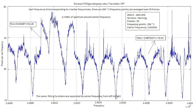
The Figure 2.4 and 2.5 provides the PSD and curve-fitting functions around carrier fre-quency for the two hypothesis.

(23)

Figure 2.4: PSD and Curve-fitting plot underH0

(24)

2.4.2 Histogram and Density Plots

The number of center frequencies is inversely related to USRP decimation rate. For in-stance, if the frequency range for scanning is δW and decimation rate isd then number of center frequencies(L) is given by L= ₆₄δW_{M S/sec}∗d 3_.

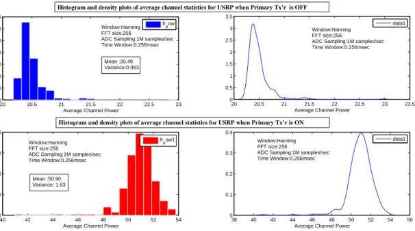
The average power for the spectrum band is the average of each average periodogram (ob-tained for each center frequency)(2.2) over the entire spectrum band. The Histogram and density plots are obtained for the average power collected over 300 frames. Histogram and density plots of average power under the two different hypotheses is shown in the Figure 2.6. The mean value in the Figure 2.6 indicates the average channel power when primary transmitter is ON (H0) and OFF(H1). In fact, the mean value of H0 is the average noise power of the channel.

20 20.5 21 21.5 22 22.5 23 0 20 40 60 80 100 120 140 Window:Hanning FFT size:256

ADC Sampling:1M samples/sec Time Window:0.256msec

Scan Count

Average Channel Power

20 20.5 21 21.5 22 22.5 23 23.5 0 0.5 1 1.5 2 2.5 3 3.5 Window:Hanning FFT size:256

40 42 44 46 48 50 52 54 0 20 40 60 80 Window:Hanning FFT size:256

Scan Count

38 40 42 44 46 48 50 52 54 56 0 0.1 0.2 0.3 0.4 Window:Hanning FFT size:256

Average Channel Power fr pow data1 data1 fr pow1 Mean :50.90 Variance: 1.63 Mean :20.49 Variance:0.063

Histogram and density plots of average channel statistics for USRP when Primary Tx’r is OFF

Histogram and density plots of average channel statistics for USRP when Primary Tx’r is ON

Figure 2.6: Histogram and density plots of average channel power for H0andH1

2.4.3 Cases

The histogram and density plots of average channel power underH1 are evaluated for dif-ferent time windows and windowing functions.

(25)

2.4.3.1 Time Window

By changing the decimation rate and FFT length, the time window of measurement is varied. In USRP ADC clock runs at 64 MS/sec.

For example, the decimation rate is 8 and FFT length =256 and the samples at ADC are decimated by factor of 8 and sampled at 8 MS/sec i.e., Time window for 256 samples is 0.256 msec.

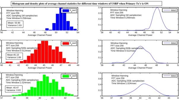
The Histogram and density plots are plotted for varying decimation rates(64,128,256) and with constant FFT length(256) is provided in the Figure 2.7.

There is decrease in the value of average channel power with the increase of time window

Scan Count

40 41 42 43 44 45 46 47 48 49 0 10 20 30 40 Window:Hanning FFT size:256

ADC Sampling:500k samples/sec Time Window:0.512msec

Scan Count

38 40 42 44 46 48 50 52 0 0.1 0.2 0.3 0.4 Window:Hanning FFT size:256

37 38 39 40 41 42 43 0 10 20 30 40 Window:Hanning FFT size:256

Scan Count

36 37 38 39 40 41 42 43 44 0 0.2 0.4 0.6 0.8 Window:Hanning FFT size:256

Average Channel Power fr pow1 fr pow2 fr pow3 data1 data1 data1 Mean:45.10 Variance:1.89 Mean: 50.90 Variance:1.63

Histogram and density plots of average channel statistics for different time windows of USRP when Primary Tx’r is ON

Mean: 40.47 Variance: 0.83

Figure 2.7: Histogram and density plots of average channel power for different time windows under H1

where the increase of time window is achieved by decreasing the ADC sampling rate.

2.4.3.2 Windowing Function

Windowing is performed to reduce smearing, spectral leakage and to preserve the amplitude of signal. The different window function doesn’t affect the shape of the power spectrum. But, there is a change in characteristics of the wave such as reduction in spectral leakage and side lobe power. Hanning window gives the best performance due to lower side lobes

(26)

[13].

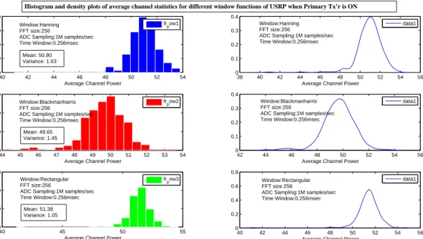
The Histogram and density plots for Hanning, Blackmanharris and Rectangular window functions is shown in the Figure 2.8.

The average channel power for different windowing functions remain constant.

Scan Count

44 45 46 47 48 49 50 51 52 53 54 0 20 40 60 Window:Blackmanharris FFT size:256

Scan Count

42 44 46 48 50 52 54 56 0 0.1 0.2 0.3 0.4 Window:Blackmanharris FFT size:256

40 45 50 55 0 50 100 150 Window:Rectangular FFT size:256

Scan Count

Average Channel Power 40 42 44 46 48 50 52 54 56 0 0.2 0.4 0.6 0.8 Window:Rectangular FFT size:256

Average Channel Power fr pow1 data1 fr pow2 data1 fr_pow3 data1 Mean: 50.90 Variance: 1.63 Mean: 49.65 Variance: 1.45 Mean: 51.38 Variance: 1.05

Histogram and density plots of average channel statistics for different window functions of USRP when Primary Tx’r is ON

Figure 2.8: Histogram and density plots of average channel power for different windowing functions underH1

2.5 Remarks

1. The bin statistics functional block performs the maximum over the dwell time for the center frequency bins. We have implemented the average over the dwell time so as to evaluate the average periodogram analysis for each center frequency.

2. The shape of the PSD determines the probability density function (pdf) of the energy statistics under each hypothesis.

3. In order to implement periodic sensing involving sleep and sensing periods, we provide sleep mode in the functional block of bin statistics. It helps to discard the samples collected during the sleep mode. It is more robust and provides efficient sensing results compared to the sleep function in python.

(27)

Chapter 3 Markov Traffic Model

3.1 Motivation

In a Cognitive Radio Network(CRN), the Markov model for the primary user(PU) spectrum usage helps to study the dynamic behavior of spectrum access and traffic patterns of the PU. Also, primary channel is modeled in the form of alternative ON and OFF cycles with secondary users (SUs) utilizing the OFF periods for transmission. For instance, a simulation model of semi-Markov traffic is considered for PUs to enhance the efficient utilization of the OFF periods by SU in [10].

3.2 Objective

• To generate Markov traffic model involving ON and OFF periods on a cognitive test-bed. Also, to configure ON periods for transmission of long and short bursts of traffic, while the OFF periods vary depending on the former period traffic burst. • Analyze the output spectrum for DBPSK modulation with spectrum analyzer and

MATLAB plot for the PSD equation provided in [14].

3.3 Implementation

This section discuss the Markov process and the implementation of Algorithm on GNU Radio. Moreover, the PSD equation is analyzed theoretical and practical verification is provided on a spectrum analyzer.

(28)

3.3.1 Markov Process

Markov process or Markov chain is paradigm of states in which the current state depends on the past states. Homogeneous Markov chain [6] has finite number of states that are independent of time, and their transition matrix P indicates the probability of transitions from one state to another. The Figure 3.1demonstrates the two state Markov model.

So and S1 are two states of Markov model with

S0 1−β

α β

1−β S1

Figure 3.1: Block Diagram for two state Markov model

Probability of transition from stateS1toS0i.e., P r[S0/S1] =S01=α Probability of transition from stateS0toS1i.e., P r[S1/S0] =S10=β Similarly,

Probability of transition from stateS0toS0andS1toS1i.e.,

P r[S0/S0] =S00= 1−α and P r[S1/S1] =S11 = 1−β

Transition matrix P for two state Markov model is given as

P = " S00 S01 S10 S11 # = " 1−α α β 1−β #

3.3.2 Explanation

The two state Markov model uses benchmark tx.py(GNU Radio example[1] ), which pro-vides packet based modulation for continuous and discrete transmission. In the program, the two states OFF (S0) and ON (S1) indicate the presence and absence of primary traffic on the channel. The S0 traffic is a period of no transmission that is produced on halting the main thread and S1 traffic is similar to continuous traffic. The states of Markov model are generated from the predefined transition matrix P and based on the current state, the burst traffic of ON and OFF periods are produced. Also, the program provides the

(29)

flexibility for allocation of number of states and available packets for ON cycles.

InS0 state, the time.sleep(txoff) function is utilized for halting the main thread of Python. The txoff represents the duration of OFF period, which depends on the former ON state i.e.,the length of previous ON burst determines the duration for the OFF period. The OFF periods are maintained longer than ON periods so as to provide sufficient transition time for switching between ON and OFF periods and to avoid the ON period creep into OFF period. Also, the longer ON periods requires longer OFF periods. For the run-time of the program, the indication of UuUu....1 _{represents the}_S

0 state.

InS1state, the ON period is modeled with probability density function(p.d.f)fTON(x), x >

0 that follow uniform distribution. The number of packets for ON period depends on avail-able packets and their prior probabilities. For instance, the availavail-able packets for ON periods arex,y,z then the Pr(x),Pr(y),Pr(z) determines the packets for the current ON state. The transmission period depends on data rate, number of packets and packet size. Also, the random selection of packets contributes for short and long bursts of traffic. For the run-time of the program, the indication of dots represents the number of packets transmitted. The algorithm in Appendix A provides the Markov traffic for the current model.

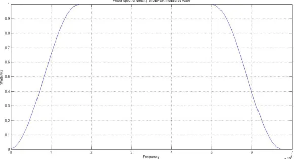
3.3.3 PSD of DBPSK Modulation

PSD for DBPSK modulated wave is given by [14]. It is based on determining the PSD for a differentially encoded sequence. DBPSK can be considered as a combination of differential encoder and BPSK modulation. The basic structure of DBPSK modulation is provided in figure 3.2. Differential Encoder ak {0,1} BPSK Modulation Vl(t) bk {0,1}

Figure 3.2: Block Diagram for DBPSK modulation

Letak be the i.i.d binary random variables with probabilities;P r[ak = 1] =pandP r[ak =

0] = 1−p; 0 < p < 1. The sequence bk is generated as bk = ak⊕ bk−1. The PSD of differentially encoded sequence(bk) and DBPSK modulated signal (Vl) is evaluated in [14]

Sb(f) = 2p(1−p) 1−(1−2p) cos 2πf T −2p(1−p)+ µ2_b T ∞ X k=−∞ δ(f−K/T) (3.1) Svl(f) = 1 T|G(f)| 2_·_S b(f) (3.2)

(30)

where,

Sb is the PSD of differential encoded sequence.

µb is the mean of the bk sequence.

G(f) is the frequency response of the pulse shape. T is the signaling interval.

If input symbols are equiprobable i.e,P r[ak = 1] = 1/2 andP r[ak = 0] = 1/2 and mean

µb = 0 then from equation (3.1)

Sb(f) = 1 (3.3)

If,g(t) is root raised cosine filter, frequency responseG(f) is provided as [6]

G(f) =        √ T for 0≤ |f| ≤ 1₂−_Tβ q T 2[1 + cos( πT β (|f| − 1−β 2T ))] for 1−β 2T ≤ |f| ≤ 1+β 2T 0 for |f| ≥ 1+₂_Tβ (3.4)

From equation (3.3) and (3.4), if the input sequence are equiprobable, the mean of differ-ential encoded sequence is zero and pulse shaping is raised cosine waveform, then PSD of DBPSK is given by (3.2) Svl(f) =      1 for 0≤ |f| ≤ 1₂−_Tβ 1 2[1 + cos( πT β (|f| − 1−β 2T ))] for 1−β 2T ≤ |f| ≤ 1+β 2T 0 for |f| ≥ 1+₂_Tβ (3.5) 3.3.3.1 Plots

The basic parameters of DBPSK modulated wave

• Roll of factor for root-raised cosine filter (β) : 0.35 • Interpolation : 128

• Carrier Frequency (fc) : 2.422 GHz

• Samples per symbol : 2

In USRP, the relation between Data rate,interpolation and samples per symbol is given as 2

Datarate(Rb) =

DACsamplingrate

Interpolation∗Samplespersymbol

For DBPSK, the symbol rate(Rs) is equal to the data rate (Rb) and the symbol period

T = 1/Rs

(31)

Substituting the value ofβand symbol periodT in equation (3.5) provides PSD for DBPSK modulation, the MATLAB plot and the output of spectrum analyzer for DBPSK modula-tion are shown in the Figures 3.3 & 3.4

Figure 3.3: MATLAB plot for PSD of DBPSK modulated waveform using equation (3.5)

(32)

3.4 Problems

Transition time is the time required to switch from one state to another. It is required to prevent the overlap between S0 and S1 periods. In fact, the longerS0 periods provides the sufficient transition time to switch between S0 and S1 periods or vice-versa. Also, the transition time from continuous S1 states to S0 state is greater than the transition time fromS0 toS1 or continuousS0 states toS1 state. For instance, the Markov chain sequence S0(1), S1(1), S0(2), S0(3), S1(2), S1(3), S1(4), S0(4), where S0(i);i = 1,2,3,4 represents OFF state and S1(i);i = 1,2,3,4 represents the ON state. The transition time between S0(1) andS1(1) orS0(3) andS1(2) is less than the transition time betweenS1(4) andS0(4). In fact, the S0(4) has longer OFF period than other OFF periods.

(33)

Chapter 4 Coded OFDM Transceiver

4.1 Motivation

Many Forward Error Correction(FEC) blocks are used with OFDM in fields such as WLAN /WMAN and DAB/DVB systems. The use of convolution codes in OFDM system helps to reduce the peak average ratio power(PARP) while improving the bit error rate (BER) [17]. In [22], a convolution code is implemented to the current OFDM model on GNU Radio that uses low code rate. However, the current Trellis Convolution Blocks on GNU Radio provide the flexibility for high code rates in addition to the Viterbi Algorithm with soft and hard decision decoding.

4.2 Objective

• Mathematical model for the Coded OFDM model

• Create Coded OFDM model using Trellis blocks in GNU Radio • Packet structure and flow for the coded OFDM model

• Cope with big burst of errors in the coded OFDM model

4.3 Implementation

This section provides the background information of OFDM model, synchronization and equalization on GNU Radio. The channel coding technique and available blocks are also

(34)

discussed. Moreover, a mathematical model for the coded OFDM is explained for the implementation.

4.3.1 Background Information

4.3.1.1 OFDM

OFDM or Orthogonal Frequency Division Multiplexing is a type of multi-carrier(MC) technique that allows for high data rate transmission and reduces the effect of Inter Symbol Interference (ISI) caused by delay spread in wireless channels [17]. It divides the available channel bandwidth (W) into sub-bands(N) of narrow-width(δf = W/N). Also, all the sub-bands are executed in parallel that are independently coded and modulated for high data rates.

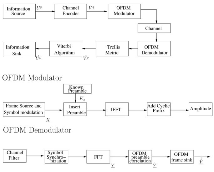
In GNU Radio, the flow-graphs for OFDM transmitter and receiver are shown in the Figure4.1.

Figure 4.1: Flow-graph for OFDM model [12]

4.3.1.2 Synchronization and Equalization

Synchronization of an OFDM signal involves finding the symbol timing and the carrier frequency offset. They need to be efficiently determined for proper recovery of OFDM symbols. In the OFDM model of Figure 4.1, signal detection at the receiver is performed using Maximum likelihood [20] or PN -sequence correlation [16]. PN- sequence correlation involves transmitting known preamble symbol along with the OFDM symbols for synchro-nization. In fact, the preamble symbol contain one training sequence with two known

(35)

symbols of equal length in the time domain.

At the transmitter, the desired training sequence is obtained from the frequency domain sequence consisting of information on even frequencies and zeros on odd frequencies which are passed through an IFFT block [12]. The generation of training sequence is demon-strated in Figure 4.2. The ”known preamble”, ”insert preamble” and ”IFFT blocks” in Figure 4.1 are responsible for generation and encapsulation of the desired training sequence. It is appended before the start of OFDM symbols that are generated from each packet.

Figure 4.2: Training Sequence for Symbol Synchronization [12]

At the receiver, the generated training sequence that is placed at the start of the packet(frame) is used for symbol synchronization. The symbol timing is achieved by searching for the symbol in which the first half is similar to second half in time domain [12]. On the other hand, equalization is achieved by generating 1-tap equalizer from the received and known symbols (training sequence) that correct phase shifts and multi-path effects. The syn-chronized and equalized OFDM symbols are passed through OFDM demodulation. In Figure 4.1, the symbol synchronization and OFDM preamble correlation blocks are used for synchronization and equalization of OFDM symbols.

4.3.1.3 Channel Coding

Convolution coding: Channel coding contains channel encoding and decoding blocks that

are used to improve the reliability of transmission by detecting and correcting errors that are introduced in the channel. Convolution coding is a type of channel coding technique that has memory and described in terms of finite state machine(FSM). In these codes, ”each time instant k, xk information is encoded to yk information sequence and changing

the state of encoded fromsk to sk−1 ” [6]. The primary advantage of convolution codes is the natural Trellis structure that helps decoding based on Viterbi algorithm.

Trellis based convolution blocks in GNU Radio: Trellis convolution blocks are based on

finite state machine(FSM). A FSM has a finite number of states,input and output sym-bols. It completely hides the information about input and output symsym-bols. In GNU Radio,

(36)

the Trellis encoder, Metric calculator and Viterbi decoder are the three blocks that uti-lize FSM structure for convolution coding. The mathematical expressions for FSM and convolution blocks are explained in the section below.

1. Trellis Encoder : It is useful for generation of encoder sequence based on the initial state of FSM.

2. Metric Calculator: It provides proper metrics to the Viterbi algorithm. The metrics can be soft or hard decision decoding, where the soft decision decoding is based on Euclidean distance and the hard decision decoding is based on Hamming distance. 3. Viterbi Decoder : It performs the Viterbi decoding for K Trellis steps.

4.3.2 Mathematical Model for Coded OFDM Blocks

Let,

• Up _and _Vq _{be the uncoded and coded bit stream of the transmitter}

• X and Y are the input and output OFDM symbol.

• N and ˜N are the FFT length and sub-carriers of the OFDM symbol. • Ks is the known preamble symbol

• Uˆp _{and ˆ}_Vq _{are the uncoded and coded bit stream of the receiver.}

• Rate of the channel encoder, e.g. code rate (p_q) = 1₂

4.3.2.1 Transmitter

The information source has data in the form of packets that are transformed into bit stream (Up_{). The bit stream is channel encoded to produce the coded bit stream(}_Vq_).

Up = (U0, U1, ..., Up−1) and Vq = (V0, V1, ..., Vq−1); Also, |Up| 6=|Vq| (4.1) where, Ui ∈ Idfori = 0,1, . . . , p−1 and Vi ∈ Odfori = 0,1, . . . , q −1 ; Id and Od are

defined from the FSM that are explained below.

(37)

Frame Source and

Symbol modulation Preamble

Insert Add Cyclic

Prefix Amplitude Preamble Channel Filter Symbol Synchro− nization FFT OFDM preamble correlation OFDM frame sink Known IFFT Information Source Channel OFDM Modulator Channel OFDM Metric Trellis Encoder Sink Information Viterbi Algorithm Demodulator Ks ´ ˆ Y

OFDM Modulator

OFDM Demodulator

X Up Vq Y Yˆ ˆ Vq ˆ Up

(38)

to sub-carriers based on the signal constellation. The output of the block is an OFDM symbol of length N which contain ˜N sub carriers and (N−N˜) zero sub-carriers.

X = (l0, l1,· · ·, lzl−1, X0, X1,· · · , XN˜−1, lzl· · · , lN−_N˜−1); |X|=N (4.2) for each sub-carrier, Xi ∈C ={aj ∈RD; 16j 6M}

where, li = 0 fori = 1,2, . . . ,(N −N˜), zl is the number of zero sub-carriers to the left

of ˜N sub-carriers, C is the constellation, aj is the signal point in C, D is the number of

dimension, M is the constellation size.

The known preamble (Ks) is appended to the OFDM symbols for synchronization and

equalization. The number of OFDM symbols between the preambles depends on packet size(mbytes),sub-carriers( ˜N) and number of bits per symbol(k).

The number of OFDM symbols generated for each packet = m_˜∗8

N∗k = 8ν, whereν = m

˜

N∗k

In fact, the output of the insert preamble block corresponds to

Ks, X0, X1,· · · , X8ν−1, Ks, X8ν, X8ν+1,· · · ·, X16ν−1· · · (4.3)

where Ks = P0Q0R0 ...

The discrete OFDM symbols(time-domain) acquired from the IFFT block are appended with the cyclic prefix.

4.3.2.2 Receiver

The output OFDM symbols of the channel are passed through the channel filter, symbol synchronization and FFT blocks to acquire the synchronized OFDM symbols(Y) based on the PN sequence correlation [12]. They are corrupted by channel coefficients(fading channel parameters) and noise.

Y = (m0, m1,· · · , mzl−1, Y0, Y1, ...YN˜−1, mzl,· · · , mN−N˜−1); |Y|=N (4.4) where,

Yk =|hk| ∗Xk+ηk, fork = 0,1, . . . ,N˜ −1

mk =|hk| ∗lk+ηk, fork = 0,1, . . . , N −N˜

|hk| and ηk are channel and noise coefficients.

The OFDM preamble correlation block performs the correlation and equalization on the synchronized OFDM symbols(Y). It accepts the vector of complex constellation points from FFT that correlates with the known preamble to estimate the frequency offset in the FFT bins. It then performs the 1-tap equalization on all the sub-carriers to correct phase and amplitude distortion. In addition, the corrupted zero sub-carriers are removed from the OFDM symbol. The algorithm for the equalization and correlation is explained

(39)

in Appendix B. ˆYis the equalized OFDM symbol. ˆ

Y = ( ˆY0,Yˆ1,· · · ,Yˆ_N˜₋₁); |Yˆ|= ˜N (4.5) where, ˆYk=Yk/hˆk=Xk+ ˆηk, ˆhk are the estimates of channel coefficients and ˆηk =ηk/hˆk.

ˆ

Y are passed through OFDM demodulator to obtain the demodulated OFDM symbols(Y´ˆ) ´

ˆ

Y = (Y´ˆ0,Y´ˆ1,· · · ,Yˆ´_N˜₋₁); |Y´ˆ|= ˜N (4.6) The algorithm for the demodulation using phase locked loop is explained in the Appendix C. The OFDM symbols are passed through the Trellis metric blocks to perform the soft or hard decision decoding so as to pass them to the Viterbi blocks.

FSM structure: All the Trellis convolution blocks are based on FSM. A FSM contains

finite number of states, input and output values. A FSM class can be constructed by con-taining information of input(I), state(S), output(O), next state(NS), output symbol(OS). They are described as

Input denotationId∈ {0,1,2· · · , I−1},with cardinality I and xk takes values fromId

Output denotationOd∈ {0,1,2· · · , O−1},with cardinalityO andyktakes values from

Od

State denotation Sd ∈ {0,1,2· · · , S−1} ,with cardinality S and sk takes values from

Sd

Next state N S :SdXId− −> Sd, meaning sk+1 =N S(sk, xk)

Output Symbol OS :SdXId− −> Od, meaning yk=OS(sk, xk)

For instance, if the code rate is 1/2, then the input cardinality(I) is 2 and the output cardinality(O) is 4. for time instant k, inputxk, statesk , output yk and yk =OS(xk, sk).

The state sk moves to the next statesk+1.

Soft Decision Decoding is based on the Euclidean Distance metric. The sub-carriers (Ykfork = 0,1,· · ·N˜−1) of synchronized OFDM symbol(Y) and their channel estimates(ˆhk)

are used in the computation.

Euclidean Distance: For each sub-carrier of D dimension, O output symbols are produced. The metrics are obtained by

kYk−hˆk∗Cik2 = D

X

j=1

|Yk,j−hˆk,j∗Ci,j|2 (4.7)

where,Yk = (Yk,1, Yk,2..., Yk,D),Ci = (Ci,1, Ci,2, ..., Ci,D) is defined from the

constel-lation, ˆhk = ( ˆhk,1,hˆk,2, ...,hk,Dˆ ) are the channel estimates for each sub-carrier and O

depends on the output cardinality of the FSM channel coder.

For instance, if the code rate= 1/2 and QPSK modulation is utilized, then the channel encoder outputs 2 bits for each 1 bit and output cardinality of FSM is 4. So, for each

(40)

sub-carrier we obtain 4 metrics i.e., for Y0, we get ||Y0−hˆ0∗C0||2,||Y0−hˆ0∗C1||2,||Y0 − ˆ

h0∗C2||2,||Y0−hˆ0∗C3||2

Hard Decision Decoding is based on the Hamming Distance metric. The sub carriers (Y´ˆkfork = 0,1,· · · ,N˜ −1) of demodulated OFDM symbol(Y´ˆ) are used in the

computa-tion.

Hamming Distance: For each sub-carrier of D dimensional vector, O output metrics are produced.The metrics are obtained by

i0 =argmin i kY´ˆk−Cik2 =argmin i D X j=1 |Y´ˆk,j−Ci,j|2 (4.8)

where Y´ˆk = (Yˆ´k,1,Y´ˆk,2...,Yk,D´ˆ ), Ci = (Ci,1, Ci,2, ..., Ci,D) are defined from the

con-stellation and O depends on the output cardinality of the FSM channel encoder. For O output metrics, the position of i0 is set to zero and the remaining metrics are taken as 1. For instance, if the code rate= 1/2 and QPSK modulation is utilized, then the channel encoder outputs 2 bits for each 1 bit and output cardinality of FSM is 4. So, for each sub-carrier we obtain 4 metrics i.e., forY´ˆ0, we get||Y´ˆ0−C0||2,||Y´ˆ0−C1||2,||Y´ˆ0−C2||2,||Y´ˆ0−C3||2 and if the value of ||Y´ˆ0 −C1||2 is minimum, then the output metrics are 1011. Since, the value of second metric is minimum, it is set to zero and the remaining three metrics are taken to be 1. These four float values corresponds to each sub-carrier that are passed through the Viterbi block.

Viterbi Algorithm Block: It instantiates the Viterbi decoder for a sequence of K trellis

epochs, whose input is a sequence of K ×O values and the output is a sequence of K values. Here, O is the output cardinality of the FSM. The output of the metric block that contains soft or hard symbols and the three metrics(PS , PI and OS ) of the FSM are utilized in decoding the K epochs.

In a p_q channel encoder, for each time instant k, input xk information is encoded to output

yk information sequence while changing the state of encoder from sk to sk−1. The three matrices provide the previous state (PS), previous input (PI) and output symbol (OS) of a FSM and each state has 2p incoming and outgoing paths. For instance, if p_q = 1₂ , then each state has 2 incoming and outgoing paths. The three matrices of the FSM are defined below.

sk−1 =P S(sk, i);i= 0,1· · ·I−1; (4.9)

xk−1 =P I(sk, i);i= 0,1· · ·I −1; (4.10)

yk =OS(sk, xk) (4.11)

where I is the input cardinality of the FSM.

(41)

stored in two vectors. In fact, the ACS (Add compare and select) algorithm is performed at each state to compute the minimum metric for all the 2p _{incoming paths.}

At the end of K epochs, the two vectors containing the minimum metric and their previ-ous state are utilized for extracting the previprevi-ous input from PI matrix. The traced path obtained from the PI matrix provides the uncoded stream.

4.4 Implementation of Coded OFDM

In all the approaches, a (2,1) trellis code with 4 state i.e, 1 bit input and two bits output is considered for channel coding. The data stream is unpacked so that each input byte into 8 single bits (carried in a byte1_{) before the trellis encoding and pack every four 2-bit worth} bytes into a single byte after trellis encoding. It implies that for every information bearing byte (before unpacking) we get two coded bytes (after packing).

4.4.1 Approach 1

4.4.1.1 Transmitter

In uncoded OFDM model, the data stream in information source is encapsulated with header and CRC, which are passed through the OFDM blocks. However, the coded OFDM model contains the channel encoder that is inserted between information source and OFDM blocks. In fact, the trellis blocks in GNU Radio which are based on FSM structure are utilized for the channel encoding. The Figure 4.4 demonstrates the flow-graph structure for the coded OFDM.

The encapsulated data stream containing header and CRC fields are traversed through the message source. The message source is a queue that contains a pointer on the top of the stack(queue). The output of the message source is connected to the ”pack-and-unpack” block to send the stream of correct input bits to the trellis encoder. The number of bits to the trellis encoder depends on the code rate. The trellis encoded stream is packed into bytes before sending into the message sink. The packet from the message sink are passed onto the OFDM blocks. Also, the message sink is a queue similar to the message source block.

In order to pass the packets from message sink onto the OFDM blocks, a separate thread runs in parallel to the main program. The primary objective of the thread is to observe the packets in the message queue and upon the reception of the packet, they are transferred

1_{In GNU Radio, the data stream is in the form of bytes and to input single bit to the trellis encoder}

(42)

Figure 4.4: Approach 1: Flow-graph for coded OFDM transmitter

to the OFDM blocks.

4.4.1.2 Receiver

Figure 4.5: Approach 1: Flow-graph for coded OFDM receiver

In the uncoded OFDM model, the OFDM demodulator block performs the symbol syn-chronization, FFT, equalization and demodulation of the OFDM symbols.In fact, the de-modulation and framing of the packets are performed in OFDM frame sink.

For the coded OFDM model, the output of the demodulated symbols (i.e., the output of OFDM frame sink block) is connected to the metrics calculator which produces the re-quired input symbols to Viterbi decoder. The Viterbi decoder obtains the uncoded packet

(43)

based on trellis steps, initial and final states of the FSM. The decoded bytes are packed and sent to the frame sink. The frame sink looks for the start of the header and packs the payload and CRC in a message queue.

4.4.2 Approach 2

4.4.2.1 Problems in Approach 1

The program doesn’t output any packets during the execution. The problem should be with the metric calculator and OFDM frame sink. In the receiver, the input to the metric calculator block should be synchronized OFDM symbols instead of demodulated symbols as soft decision decoding is implemented in the metric block. The possible approach is to output the soft symbols of the preamble correlation to the metric calculation and perform Viterbi decoding for the acquired soft symbols.

Figure 4.6: Approach 2: Flow-graph for coded OFDM receiver

4.4.2.2 Receiver

In the present approach, the output of the OFDM preamble correlation block, which pro-vides the symbol and phase synchronized OFDM symbols are connected directly to the trellis metric block.The correlation block has two outputs. One to pass the streams of OFDM symbols, while the other contains the flag to indicate the start of OFDM symbols. The metric block is structured to perform soft decision decoding for the OFDM symbols when it receives the flag output. The corresponding metric values are passed to the Viterbi

(44)

block and then moved to the frame sink for determining the packet loss rate. The approach has more than 90 % packet loss.

4.4.3 Approach 3 : Working Model

Problem:

The receiver and packet structure are the main problems of the former approach. The demodulated OFDM symbols which enter the trellis metric are in disarray with the trans-mitted OFDM symbols (i.e., OFDM symbols produced by each packet on the transmitter are not properly aligned at the receiver). Moreover, the header and CRC fields are incor-rectly detected in the frame sink.

Approach:

• In order to design the coded OFDM model, the ”equivalent inner channel” created between the trellis encoder and the Viterbi decoder, including the packing/message queuing/ofdm modulation/demodulation, etc, up until the input to the metric cal-culation block should be working perfectly. This ”equivalent inner channel” has to be a byte-in byte-out channel, where each byte is carrying only 2 bits 2. The metrics defined are ”symbol-wise Hamming distance” i.e., to perform Hard Decision Decod-ing.

• The header and CRC fields are added to the coded data stream and the frame sink is replaced by message sink.

4.4.3.1 Transmitter

The flow-graph structure is similar to the Figure 4.4. The only difference is the encapsu-lation of header and CRC fields. The coded data stream in the message sink is appended with header and CRC fields that are sent to the OFDM modulator blocks.

4.4.3.2 Receiver

For coded OFDM system, the coded packets after the removal of header and CRC are passed on to a message source. They are passed through a unpack block to provide ap-propriate input bits to trellis metric (to perform Hard Decision Decoding) and produce required input symbols to Viterbi decoder to obtain the uncoded packet based on trellis

2_{In GNU Radio, the data stream is in form of bytes and here each byte for the inner channel contains}

(45)

Figure 4.7: Working Model: Flow-graph for coded OFDM receiver

steps, finite state machine initial and final states. The decoded bytes consisting of payload and CRC are packed and sent to a message sink.

Two separate threads are created. One passes the coded packets from the output of mes-sage queue of OFDM frame sink onto the mesmes-sage source block. The other thread is used to perform the detection of received packets in the message sink.

4.5 Packet Structure and Packet Flow for Coded OFDM

4.5.1 Packet Structure

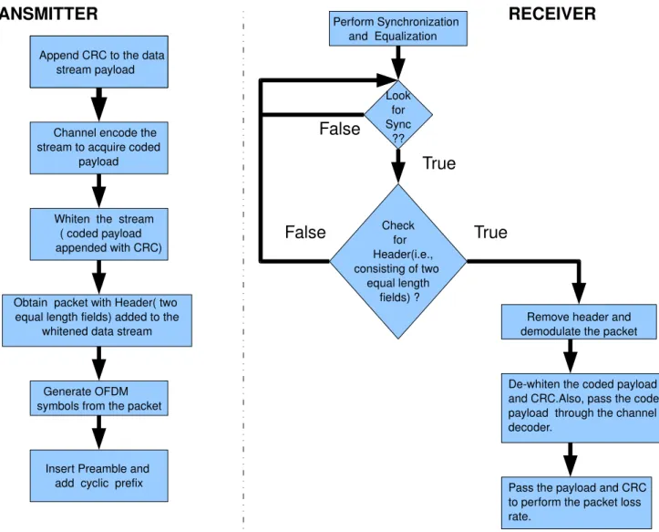
The three fields of the packet structure are header, coded payload and CRC. The header contains two equal length fields that comprises offset and coded payload length. The two equal length fields are used for identifying the packet at the receiver. The coded payload is acquired through the channel encoder. The channel encoder in the figure 4.8 is a FSM convolution encoder, which is discussed in the section above. The CRC field is used for Forward error correction (FEC) of packets at the receiver. Moreover, the coded payload and CRC fields are whitened, which involves bit-wise XOR operation with pseudo random stream of data. The packet structure for the coded OFDM model is shown in the Figure 4.8.

(46)

Payload CRC Channel _Encoder Coded_payload

Header Coded_Payload CRC 4 bytes 4 bytes

Offset coded_payload_Length

4

bits 12 bits 4 bits

12 bits 4 bytes Payload is from generated data stream and each coded_payload are independent; i.e., no correlation between two coded_payload streams. Whitened (scrambled)

Figure 4.8: Packet structure for coded OFDM model

4.5.2 Packet Flow

4.5.2.1 Transmitter

• Step 1: Append CRC to the data stream payload. The payload is obtained from the information source(ex: binary or image file for transmission).

• Step 2: Channel encode the stream to acquire the coded payload. The encoded stream depends on the code rate.

• Step 3: Whiten(scramble) the data stream (coded payload appended with CRC). It involves bit-wise XOR operation with known PN-sequence.

• Step 4: Generate header(4 bytes) of two equal 2 bytes consisting of offset(upper nibble) and coded payload length(12 bits); Add header to the whitened data stream and pack them into packets, and send to the message queue.

• Step 5: Generate OFDM symbols from packets based on number of sub-carriers and signal constellation.

• Step 6: Insert known preamble; In the time domain it corresponds to one training symbol consisting of two equal length symbols.

(47)

Look for Sync ?? Perform Synchronization and Equalization Check for Header(i.e., consisting of two equal length fields) ? True Dewhiten the coded payload and CRC.Also, pass the coded payload through the channel decoder. Pass the payload and CRC to perform the packet loss rate. False Obtain the payload from data stream and append with CRC Channel encode the stream to acquire coded payload Whiten the stream ( coded payload appended with CRC) Obtain packet with Header( two equal length fields) added to the whitened data stream Generate OFDM symbols from the packet Insert Preamble and add cyclic prefix Append CRC to the data stream payload TRANSMITTER RECEIVER True False Remove header and demodulate the packet

(48)

4.5.2.2 Receiver

• Step 1: Perform synchronization and equalization [16].

• Step 2: Look for the sync signal i.e., an indicator for start of the packet. • Step 3: Check for the header with two equal length fields.

• Step 4: Remove the header and demodulate the OFDM symbols.

• Step 5: De-whiten the payload and CRC and pack coded payload into packets. • Step 6: Pass the packet through a channel decoder to obtain payload and CRC. • Step 7: Calculate the packet loss rate.

4.6 Problems

4.6.1 Cope with Big Burst of Errors in Coded OFDM Model

• Modified Header

Problem: The data stream(payload) is passed through the channel encoder to acquire

the coded payload. Each coded payload is independent i.e., there is no correlation between two coded payload streams. The coded payload is added with header and CRC before passing through the OFDM blocks. At the receiver, the demodulated OFDM symbols look for the header with two equal length fields. As a result, any false alarm of the header(incorrect header containing two equal length fields) leads to misalignment of the channel decoder with a complete loss of packets.

Approach: The header field has two equal length fields. We included the two bit

parity for each field that can be used for error detection. In fact, the header size is maintained to be 4 bytes by shortening the offset size to 2 bits. This reduces the overhead of additional bits in the header. Moreover, the receiver is designed for header verification of two equal length fields and parity check bit. This prevents the header mismatch and packet loss. The modified packet structure is shown in the Figure 4.10.

• Interleaving

Appending convolution interleaving to the coded data stream reduce the burst of errors. The interleaver is attached to the output of the trellis encoder while the de-interleaver to the input of the trellis metric.

• Packet size

Reducing the packet size of transmission. In fact, the trellis encoder and decoder per-form better for smaller trellis steps. As a result, transmission of packets in smaller

(49)

Payload CRC Channel Encoder Coded_payload Header Coded_Payload CRC 4 bytes 4 bytes Parity_

check coded_payloadLength

2 bits 12 bits 4 bytes Payload is from generated data stream and each coded_payload are independent; i.e., no correlation between two coded_payload streams. Whitened (scrambled) Offset 2 bits Parity_

check coded_payloadLength

2 bits 12 bits

Offset

2 bits

Figure 4.10: Modified Header Packet Structure

size decreases packet loss rate.

For instance, payload1 and payload2 are two equal length data stream, then payload1 + CRC through channel encoder has less than 1% packet loss and payload1+payload2+CRC stream through channel encoder has 50 to 60% packet loss. The packet loss rate is decreased with smaller packet size.

• Sleep function

The use of sleep function(time.sleep()) in the queue watcher threads helps to protect the integrity of packets for trellis decoding. Two threads are watched at the receiver, one observes the message queue of the ofdm frame sink block to pass the data stream through channel decoder and the other thread is used to watch the output stream of the channel decoder to perform FEC(CRC check) and measure the packet loss rate. The packets for the second thread are obtained from the channel decoded stream of messages of first thread. So, the second thread is provided some transition time (time.sleep(0.01)) to reduce the packet loss rate.

4.6.2 Remarks

1. There is a significant packet loss in OFDM at the receiver due to mis-match on the preamble and miss the entire packet. The problem in capturing some of the packets seems to be at the ofdm sync blocks in the receiver. As a result, the headers are

Experimental study of cognitive radio test-bed using USRP

Louisiana State University

LSU Digital Commons

Experimental study of cognitive radio test-bed

using USRP

Venkat vinod Patcha

EXPERIMENTAL STUDY OF COGNITIVE RADIO TEST-BED USING USRP

Acknowledgments

Table of Contents

List of Tables

List of Figures

Abstract

Chapter 1

Introduction

1.1

Motivation

1.2

Contribution of Thesis

1.3

Background Information for Test-Bed Model

1.3.1

Hardware: USRP (Universal Software Radio Peripheral)

1.3.2

Software: GNU Radio

1.4

Organization of Thesis

Chapter 2

Spectrum Sensing of Primary User

2.1

Motivation

2.2

Objective

2.3

Implementation

2.3.1

Average Periodogram Analysis

2.3.2

Wide-band Spectrum Analyzer for USRP

2.3.3

Methodology

2.4

Analysis

2.4.1

PSD and Curve-fitting Functions

2.4.2

Histogram and Density Plots

2.4.3

Cases

2.5

Remarks

Chapter 3

Markov Traffic Model

3.1

Motivation

3.2

Objective

3.3

Implementation

3.3.1

Markov Process

3.3.2

Explanation

3.3.3

PSD of DBPSK Modulation

3.4

Problems

Chapter 4

Coded OFDM Transceiver

4.1

Motivation

4.2

Objective

4.3

Implementation

4.3.1

Background Information

4.3.2

Mathematical Model for Coded OFDM Blocks

OFDM Modulator

OFDM Demodulator