2018
First-order methods of solving nonconvex
optimization problems: Algorithms, convergence,
and optimality
Songtao Lu
Iowa State UniversityFollow this and additional works at:
https://lib.dr.iastate.edu/etd
Part of the
Electrical and Electronics Commons
This Dissertation is brought to you for free and open access by the Iowa State University Capstones, Theses and Dissertations at Iowa State University Digital Repository. It has been accepted for inclusion in Graduate Theses and Dissertations by an authorized administrator of Iowa State University Digital Repository. For more information, please [email protected].
Recommended Citation
Lu, Songtao, "First-order methods of solving nonconvex optimization problems: Algorithms, convergence, and optimality" (2018). Graduate Theses and Dissertations. 16628.
Algorithms, convergence, and optimality
by
Songtao Lu
A dissertation submitted to the graduate faculty in partial fulfillment of the requirements for the degree of
DOCTOR OF PHILOSOPHY
Major: Electrical Engineering
Program of Study Committee: Mingyi Hong, Co-major Professor Zhengdao Wang, Co-major Professor
Nicola Elia Aleksandar Dogandˇzi´c
Kris De Brabanter
The student author, whose presentation of the scholarship herein was approved by the program of study committee, is solely responsible for the content of this dissertation. The Graduate College will ensure this dissertation is globally accessible and will not permit alterations after a degree is
conferred.
Iowa State University Ames, Iowa
2018
TABLE OF CONTENTS
Page
LIST OF TABLES . . . vi
LIST OF FIGURES . . . vii
ABSTRACT . . . ix
CHAPTER 1. OVERVIEW . . . 1
1.1 Constrained Nonconvex Problems . . . 1
1.1.1 Symmetric Nonnegative Matrix Factorization . . . 1
1.1.2 Stochastic SymNMF . . . 2
1.2 Unconstrained Nonconvex Problems . . . 3
1.2.1 Perturbed Alternating Gradient Descent . . . 4
CHAPTER 2. SYMMETRIC NONNEGATIVE MATRIX FACTORIZATION . . . 6
2.1 Introduction . . . 6
2.1.1 Related Work . . . 6
2.1.2 Contributions . . . 8
2.2 NS-SymNMF . . . 9
2.3 Convergence Analysis . . . 12
2.3.1 Convergence and Convergence Rate . . . 12
2.3.2 Sufficient Global and Local Optimality Conditions . . . 13
2.3.3 Implementation . . . 15
2.4 Numerical Results . . . 16
2.4.1 Algorithms Comparison . . . 17
2.4.2 Performance on Synthetic Data . . . 19
2.4.4 Performance on Real Data . . . 22
CHAPTER 3. STOCHASTIC SYMMETRIC NONNEGATIVE MATRIX FACTORIZATION 26 3.1 Introduction . . . 26
3.2 Stochastic Nonconvex Splitting for SymNMF . . . 27
3.2.1 Main Assumptions . . . 27
3.2.2 The Problem Formulation for Stochastic SymNMF . . . 28
3.2.3 The Framework of SNS for SymNMF . . . 29
3.2.4 Implementation of the SNS-SymNMF Algorithm . . . 30
3.3 Convergence Analysis . . . 30
3.4 Numerical Results . . . 32
3.4.1 Synthetic Data Set . . . 32
3.4.2 Real Data Set . . . 36
CHAPTER 4. PERTURBED ALTERNATING GRADIENT DESCENT . . . 38
4.1 Introduction . . . 38
4.1.1 Scope of This Work . . . 39
4.1.2 Contributions . . . 40
4.2 Preliminaries . . . 41
4.2.1 Definitions . . . 41
4.3 Perturbed Alternating Gradient Descent . . . 42
4.3.1 Algorithm Description . . . 42
4.3.2 Convergence Rate Analysis . . . 44
4.4 Perturbed Alternating Proximal Point . . . 45
4.5 Convergence Analysis . . . 47
4.5.1 The Main Difficulty of the Proof . . . 47
4.5.2 The Main Idea of the Proof . . . 48
4.5.3 The Sketch of the Proof . . . 49
4.6 Connection with Existing Works . . . 52
4.7 Numerical Results . . . 53
4.7.1 A Simple Example . . . 53
4.7.2 Asymmetric Matrix Factorization (AMF) . . . 53
CHAPTER 5. CONCLUSION . . . 56
BIBLIOGRAPHY . . . 58
APPENDIX A. SOME PROOFS OF SYMNMF . . . 71
A.1 Proof of Lemma1 . . . 71
A.2 Proof of Lemma2 . . . 72
A.3 Convergence Proof of the NS-SymNMF Algorithm . . . 73
A.4 Convergence Rate Proof of the NS-SymNMF Algorithm . . . 79
A.5 Sufficient Condition of Optimality of SymNMF . . . 82
A.6 Sufficient Local Optimality Condition . . . 83
A.7 Sufficient Local Optimality Condition WhenK= 1 (The proof of Corollary 1) . . . 85
APPENDIX B. PROOFS OF PA-GD . . . 87
B.1 Proofs of the Preliminary Lemmas . . . 87
B.1.1 Proof of Lemma11 . . . 88
B.1.2 Proof of Lemma12 . . . 88
B.1.3 Proof of Lemma13 . . . 89
B.2 Proofs of the Convergence Rate of PA-GD . . . 90
B.2.1 Proof of Theorem 8 . . . 93 B.2.2 Proof of Lemma4 . . . 95 B.2.3 Proof of Lemma5 . . . 98 B.2.4 Proof of Lemma14 . . . 99 B.2.5 Proof of Lemma15 . . . 102 B.2.6 Proof of Lemma16 . . . 111
B.3.1 Proof of Corollary3 . . . 118 B.3.2 Proof of Corollary4 . . . 120 B.3.3 Proof of Lemma17 . . . 123 B.3.4 Proof of Lemma18 . . . 123 B.3.5 Proof of Lemma19 . . . 125 B.3.6 Proof of Lemma20 . . . 125 B.3.7 Proof of Lemma21 . . . 126 B.3.8 Proof of Lemma22 . . . 134 B.4 Proof of Lemma7 . . . 134
LIST OF TABLES
Page Table 2.1 Local Optimality . . . 21
Table 2.2 Mean and Standard Deviation ofkXXT−Zk2
F/kZk2F Obtained by the Final
Solution of Each Algorithm based on Random Initializations (dense similar-ity matrices) . . . 23
Table 2.3 Mean and Standard Deviation ofkXXT −Zk2
F/kZk2F Obtained by the
Fi-nal Solution of Each Algorithm based on Random Initializations (sparse similarity matrices) . . . 24
Table 3.1 Rules of Aggregating Samples . . . 28
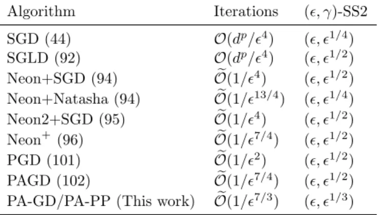
Table 4.1 Convergence rates of algorithms to SS2 with the first order information, wherep≥4, andOe hides factor ploylog(d). . . 39
LIST OF FIGURES
Page Figure 2.1 Data Set I: the convergence behaviors of different SymNMF solvers. . . 20
Figure 2.2 Data Set II: the convergence behaviors of different SymNMF solvers; N = 2000,K = 4. . . 20
Figure 2.3 Checking local optimality condition, whereN = 500. . . 21
Figure 2.4 The convergence behaviors of different SymNMF solvers for the dense sim-ilarity matrix. . . 22
Figure 2.5 The convergence behaviors of different SymNMF solvers for the sparse sim-ilarity matrix. . . 24
Figure 3.1 The convergence behaviors. The parameters are K = 4; N = 120; L = 10. The
x-axis represents the total number of observed samples. . . 33
Figure 3.2 The convergence behaviors. The parameters areK = 4; N = 120; L= 10. Thex-axis represents the total number of the observed samples for stochastic SymNMF and iterations for deterministic SymNMF. . . 35
Figure 3.3 The convergence behaviors. The parameters areK = 5; N = 240; L= 10. The x-axis represents the total number of observed samples for stochastic SymNMF and iterations for deterministic SymNMF. . . 35
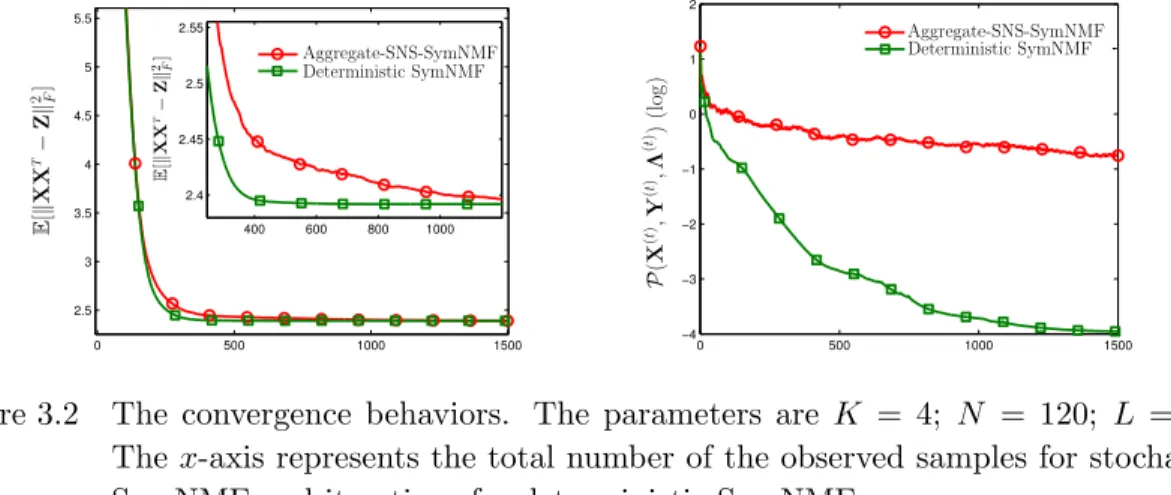
Figure 4.1 Contour of the objective values and the trajectory (pink color) of PA-GD started near strict saddle point [0,0]. The objective function is f(x) = xTAx,x= [x
1;x2]∈R2×1 whereA := [1 2; 2 1]∈R2×2, and the length of the arrows indicate the strength of −∇f(x) projected onto directions x1,x2. . . 44
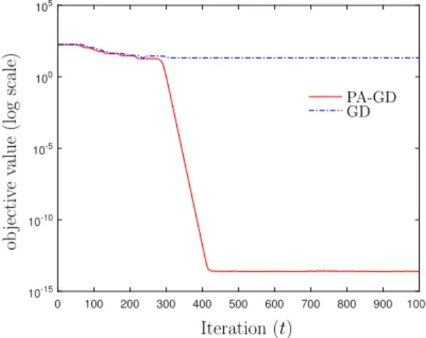
Figure 4.2 Convergence comparison between AGD and PA-GD, where = 10−4,g
th =
/10,η= 0.02, tth = 10/1/3,r =/10. . . 54
Figure 4.3 Convergence comparison between AGD and PA-GD for asymmetric matrix factorization, where = 10−14, g
th = /10, η = 6×10⁻³, tth = 10/1/3,
ABSTRACT
First-order methods for solving large scale nonconvex problems have been applied in many areas of machine learning, such as matrix factorization, dictionary learning, matrix sensing/completion, training deep neural networks, etc. For example, matrix factorization problems have lots of im-portant applications in document clustering, community detection and image segmentation. In this dissertation, we first study some novel nonconvex variable splitting methods for solving some matrix factorization problems, mainly focusing on symmetric non-negative matrix factorization (SymNMF) and stochastic SymNMF.
In the problem of SymNMF, the proposed algorithm, called nonconvex splitting SymNMF (NS-SymNMF), is guaranteed to converge to the set of Karush-Kuhn-Tucker (KKT) points of the nonconvex SymNMF problem. Furthermore, it achieves a global sublinear convergence rate. We also show that the algorithm can be efficiently implemented in a distributed manner. Further, sufficient conditions are provided which guarantee the global and local optimality of the obtained solutions. Extensive numerical results performed on both synthetic and real data sets suggest that the proposed algorithm converges quickly to a local minimum solution.
Furthermore, we consider a stochastic SymNMF problem in which the observation matrix is generated in a random and sequential manner. The proposed stochastic nonconvex splitting method not only guarantees convergence to the set of stationary points of the problem (in the mean-square sense), but further achieves a sublinear convergence rate. Numerical results show that for clustering problems over both synthetic and real world datasets, the proposed algorithm converges quickly to the set of stationary points.
When the objective function is nonconvex, it is well-known the most of the first-order algorithms converge to the order stationary solution (SS1) with a global sublinear rate. Whether the first-order algorithm can converge to the second-first-order stationary points (SS2) with some provable rate
has attracted a lot of attention recently. In particular, we study the alternating gradient descent (AGD) algorithm as an example, which is a simple but popular algorithm and has been applied to problems in optimization, machine learning, data mining, and signal processing, etc. The algorithm updates two blocks of variables in an alternating manner, in which a gradient step is taken on one block, while keeping the remaining block fixed.
In this work, we show that a variant of AGD-type algorithms will not be trapped by “bad” stationary solutions such as saddle points and local maximum points. In particular, we consider a smooth unconstrained nonconvex optimization problem, and propose a perturbed AGD (PA-GD) which converges (with high probability) to the set of SS2 with a global sublinear rate. To the best of our knowledge, this is the first alternating type algorithm which is guaranteed to achieve SS2 points with high probability and the corresponding convergence rate is O(polylog(d)/7/3) [where polylog(d) is polynomial of the logarithm of problem dimension d].
CHAPTER 1. OVERVIEW
In this dissertation, we study nonconvex optimization problems in both constrained and un-constrained cases. For the un-constrained case, we consider the symmetric nonnegative matrix fac-torization (SymNMF) as an example. We propose a nonconvex splitting algorithm and study the convergence behaviour of the algorithm. Also, the optimality condition of the obtained solutions for this problem is provided, which verifies the quality of the obtained solutions. Furthermore, the stochastic SymNMF is also considered, where the corresponding stochastic nonconvex splitting algorithm is proposed as well. In the unconstrained nonconvex optimization case, there are many nonconvex optimization problems where the saddle points of the objective functions are strict and local optimal points are also global ones. Then, a perturbed alternating gradient descent algorith-m is proposed for solving a class of block structured nonconvex optialgorith-mization problealgorith-ms. Finally, under some mild assumptions, we will show that the proposed algorithm is able to converge to the second-order stationary points (SS2) with high probability in a sublinear rate.
1.1 Constrained Nonconvex Problems
1.1.1 Symmetric Nonnegative Matrix Factorization
Non-negative matrix factorization (NMF) refers to factoring a given matrix into the product of two matrices whose entries are all non-negative. It has long been recognized as an important matrix decomposition problem (1; 2). The requirement that the factors are component-wise nonnegative makes the NMF distinct from traditional methods such as the principal component analysis (PCA) and latent dirichlet allocation (LDA), leading to many interesting applications in imaging, signal processing and machine learning (3; 4; 5; 6; 7); see (8) for a recent survey. When further requiring that the two factors are identical after transposition, the NMF becomes the so-called SymNMF. In the case where the given matrix cannot be factorized exactly, an approximate solution with
a suitably defined approximation error is desired. Mathematically, the SymNMF approximates a given (usually symmetric) non-negative matrix Z∈RN×N by a low rank matrixXXT, where the
factor matrix X ∈RN×K is component-wise non-negative, typically with K N. Such problem
can be formulated as the following nonconvex optimization problem (9; 10; 11): min X≥0 1 2kXX T −Zk2F (1.1)
wherek · kF denotes the Frobenius norm and inequality constraintX≥0 is component-wise.
Recently, SymNMF has found many applications in document clustering, community detection, image segmentation and pattern clustering in bioinformatics (11; 12; 13; 9). An important class of clustering methods is known as the spectral clustering, e.g., (14; 15), which is based on the eigen-value decomposition of some transformed graph Laplacian matrix. In (16), it has been shown that spectral clustering and SymNMF are two different ways of relaxing the kernelK-means clustering, where the former relaxes the nonnegativity constraint while the latter relaxes certain orthogonality constraint. Furthermore, SymNMF has the advantage that it often yields more meaningful and interpretable results (11). In this work, a new nonconvex splitting method is proposed which is an efficient way of solving SymNMF problems with provable convergence guarantees.
1.1.2 Stochastic SymNMF
Classical SymNMF problems in the data mining area are deterministic, where the observation matrix Z is completely known (11; 17). However, in recent applications such as social network community detection, the matrix Z represents the relations among the clusters/communities, ob-served during a given time period. By nature such matrix is random, whose structure is determined by the dynamics of the network connections (18). Furthermore, in many modern big-data related problems such as matrix completion (19), subspace tracking (20), community detection, the data are usually collected through some random sampling techniques. As a concrete example, in com-munity detection problems the observed activities among the nodes can change over time hence is random. In these applications sampling the connectivity of the graph at a given time results in a random similarity matrix, such as stochastic block model (21). Mathematically, the stochastic
SymNMF problem can be formulated as the following stochastic optimization problem min X≥0 1 2EZ[kXX T −Zk2F] (1.2)
where Z follows some distribution over a set Ξ ∈ RN×N, and the expectation is taken over the
random observation Z. In clustering problems, the samples of matrix Z can be the similarity matrix which measures the connections among nodes over networks.
As we will see later, the problem in (1.1) is equivalent to minX≥0kXXT −EZ[Z]k2F. If we
know the distribution of Z, then we can computer EZ[Z] first and the problem is converted to a
classical SymNMF problem. However, in practice, we usually do not have access to the underlying distribution ofZ. Instead, we can obtain sequentially realizations ofZ, such as in the application of online streaming data (22). It is possible to use a batch of samples to compute the empirical mean of Zand implement the deterministic SymNMF algorithms. As more samples are collected, the empirical mean will converge to the ensemble mean, leading to a consistent estimator of the solution of the symmetric factorX. There are two problems with such an approach. First, it may be desirable to have an estimate of the symmetric factor X at each time instant, namely when a new sample of Z is available. Running the complete SymNMF algorithm at each time instant may be computationally expensive. Second, even if the computational complexity is not a concern, existing analysis results and theoretical guarantees such as convergence rate are not applicable to the case where the matrix to be factorized is changing with time (although eventually converging to the ensemble mean). Therefore, it is desirable to develop efficient algorithms that produce online SymNMF updates based on sequential realizations ofZ.
1.2 Unconstrained Nonconvex Problems
Although the constrained nonconvex problems have been solved efficiently, these first-order can only guraantee that the generated squence by the algorithms converge to the first-order stationary points (SS1). In recent works, it has been shown that with some new techniques, such as adding some perturbation on the iterates of the algorithm occasionally, the first-order algorithms can converge to second-order stationary points (SS2) efficiently. In this work, we take one of the most
popular algorithm, alternating gradient descent (AGD), as example and study the convergence behaviour of this algorithm to SS2.
1.2.1 Perturbed Alternating Gradient Descent
We consider a smooth and unconstrained nonconvex optimization problem min
x∈Rd×1f(x) (1.3)
wheref :Rd→Ris twice differentiable. Problem (1.3) is a general formulation in most of machine
learning topics, such as matrix factorization-type of problems (23; 24), regression problems (25), deep learning problems (26).
There are many ways of solving problem (1.3), such as gradient descent (GD), accelerated gradient descent (AGD), etc. When the problem dimension is large, it is natural to split the variables into multiple blocks and solve the subproblems with smaller size individually. The block coordinate descent (BCD) algorithm, and many of its variants such as block coordinate gradient descent (BCGD) and alternating gradient descent (AGD) (27; 28), are among the most powerful tools for solving large scale convex/nonconvex optimization problems (29; 30; 31; 32; 33). The BCD-type algorithms partition the optimization variables into multiple small blocks, and optimize each block one by one following certain block selection rule, such as cyclic rule (34), Gauss-Southwell rule (35), etc. To be more specific, problem (1.3) can be solved by the following reformulation.
min
xk
f(x1, . . . ,xk, . . . ,xK), k= 1, . . . , K (1.4)
wherek denotes the index of the blocks, andK denotes the total number of blocks.
In recent years, there are many applications of BCD-type algorithms in the areas of machine learning and data mining, such as matrix factorization (36), tensor decomposition, low rank matrix estimation (37; 23), matrix completion/sensing (19), and training deep neural networks (DNNs) (38). Under relatively mild conditions, the convergence of BCD-type algorithms to SS1 have been broadly investigated for nonconvex and non-differentiable optimization (34; 39; 40). In particular, it is known that under mild conditions, these algorithms also achieve global sublinear rates (41).
However, despite its popularity and significant recent progress in understanding its behavior, it remains unclear whether BCD-type algorithms can converge to the set of SS2 with a provable global rate, even for the simplest problem with two blocks of variables.
Algorithms that can escape from strict saddle points – those stationary points that have negative eigenvalues – have wide applications. Many recent works have analyzed the saddle points in machine learning problems (42). Such as learning in shallow networks, the stationary points are either global minimum points or strict saddle points. In two-layer porcupine neural networks (PNNs), it has been shown that most local optima of PNN optimizations are also global optimizers (43). Previous work in (44) has shown that the saddle points in tensor decomposition are indeed strict saddle points. Also, it has been shown that any saddle points are strict in dictionary learning and phase retrieval problems theoretically (45; 46) and numerically in (47). More recently, (24) proposed a unified analysis of saddle points for a board class of low rank matrix factorization problems, and they proved that these saddle points are strict.
Motivated by these results, we will show that AGD with some random perturbation can still converge to SS2 efficiently for unconstrained nonconvex optimization problems in a global sublinear convergence rate.
CHAPTER 2. SYMMETRIC NONNEGATIVE MATRIX FACTORIZATION
2.1 Introduction
Due to the importance of the NMF problem, many algorithms have been proposed in the litera-ture for finding its high-quality solutions. Well-known algorithms include the multiplicative update (6), alternating projected gradient methods (48), alternating nonnegative least squares (ANLS) with the active set method (49) and a few recent methods such as the bilinear generalized approx-imate message passing (50; 51), as well as methods based on the block coordinate descent (52). These methods often possess strong convergence guarantees (to Karush-Kuhn-Tucker (KKT) points of the NMF problem) and most of them lead to satisfactory performance in practice; see (8) and the references therein for detailed comparison and comments for different algorithms. Unfortunately, most of the aforementioned methods for NMF lack effective mechanisms to enforce the symmetry between the resulting factors, therefore they are not directly applicable to the SymNMF. Recently, there have been a number of works that focus on designing customized algorithms for SymNMF, which we review below.
2.1.1 Related Work
To this end, first rewrite the SymNMF equivalently as min Y≥0,X=Y 1 2kXY T −Zk2 F. (2.1)
A simple strategy is to ignore the equality constraint X=Y, and then alternatingly perform the following two steps: 1) solving Y with X being fixed (a non-negative least squares problem); 2) solvingXwith Y being fixed (a least squares problem). Such ANLS algorithm has been proposed in (11) for dealing with SymNMF. Unfortunately, despite the fact that an optimal solution can be obtained in each subproblem, there is no guarantee that theY-iterate will converge to the X -iterate. The algorithm in (11) adds a regularized term for the difference between the two factors to
the objective function and explicitly enforces that the two matrices be equal at the output. Such an extra step enforces symmetry, but unfortunately also leads to the loss of global convergence guarantee. A related ANLS-based method has been introduced in (10); however the algorithm is based on the assumption that there exists an exact symmetric factorization (i.e., ∃ X ≥ 0 such XXT =Z). Without such assumption, the algorithm may not converge to the set of KKT points1 of (1.1). A multiplicative update for SymNMF has been proposed in (9), but the algorithm lacks convergence guarantee (to KKT points of (1.1)) (53), and has a much slower convergence speed than the one proposed in (10). In (11; 54), algorithms based on the projected gradient descent (PGD) and the projected Newton (PNewton) have been proposed, both of which directly solve the original formulation (1.1). Again there has been no global convergence analysis since the objective function is a nonconvex fourth-order polynomial. More recently, the work (55) applies the nonconvex coordinate descent (CD) algorithm for SymNMF. However, due to the fact that the minimizer of the fourth order polynomial is not unique in each coordinate updating, the CD-based method may not converge to stationary points.
Another popular method for NMF is based on the alternating direction method of multipliers (ADMM), which is a flexible tool for large scale convex optimization (56). For example, using ADMM for both NMF and matrix completion, high quality results have been obtained in (57) for gray-scale and hyperspectral image recovery. Furthermore, ADMM has been applied to generalized versions of NMF where the objective function is the general beta-divergence (58). A hybrid alter-nating optimization and ADMM method was proposed for NMF, as well as tensor factorization, under a variety of constraints and loss measures in (59). However, despite the promising numerical results, none of the works discussed above has rigorous theoretical justification for SymNMF. Tech-nically, imposing symmetry poses much difficulty in the analysis (we will comment on this point shortly). In fact, the convergence of ADMM for SymNMF is still open in the literature.
An important research question for NMF and SymNMF is whether it is possible to design algorithms that lead to globally optimal solutions. At the first sight such problem appears very
1
Letd(a, s) denote the distance between two pointsaands. We say that a sequenceaiconverges to a setS if the
challenging since finding the exact NMF is NP-hard (60) and checking whether a positive semidefi-nite matrix can be decomposed exactly by SymNMF is also NP-hard (61). However, some promising recent findings suggest that when the structure of the underlying factors are appropriately utilized, it is possible to obtain rather strong results. For example, in (62), the authors have shown that for the low rank factorized stochastic optimization problem where the two low rank matrices are symmetric, a modified stochastic gradient descent algorithm is capable of converging to a glob-al optimum with constant probability from a random starting point. Related works glob-also include (63; 64; 36). However, when the factors are required to be non-negative and symmetric, it is no longer clear whether the existing analysis can still be used to show convergence to global optimal points, even local optimality (a milder result). For the non-negative principal component problem (that is, finding the leading non-negative eigenvector, i.e.,K= 1), under the spiked model, reference (65) shows that certain approximate message passing algorithm is able to find the global optimal solution asymptotically. Unfortunately, this analysis does not generalize to an arbitrary symmetric observation matrix with a larger K. To our best knowledge, there is a lack of characterization of global and local optimal solutions for the SymNMF problem.
2.1.2 Contributions
In this work, we first propose a novel algorithm for the SymNMF, which utilizes nonconvex splitting and is capable of converging to the set of KKT points with provable global convergence rate. The main idea is to relax the symmetry requirement at the beginning and gradually enforce it as the algorithm proceeds. Second, we provide a number of easy-to-check sufficient conditions guaranteeing the local or global optimality of the obtained solutions. Numerical results on both synthetic and real data show that the proposed algorithm achieves fast and stable convergence (often to local minimum solutions) with low computational complexity.
1) We design a novel algorithm, named the nonconvex splitting SymNMF (NS-SymNMF), which converges to the set of KKT points of SymNMF with a global sublinear rate. To our best knowledge, it is the first SymNMF solver that possesses global convergence rate guarantee.
2) We provide a set of easily checkable sufficient conditions (which only involve finding the smallest eigenvalue of certain matrix) that characterize the global and local optimality of the SymNMF. By utilizing such conditions, we demonstrate numerically that with high probability, our proposed algorithm converges not only to the set of KKT points but to a local optimal solution as well.
Notation: Bold upper case letters without subscripts (e.g., X,Y) denote matrices and bold lower case letters without subscripts (e.g., x,y) represent vectors. The notation Zi,j denotes the
(i, j)-th entry of the matrixZ. The vectorXi denotes theith row of the matrixXandX0mdenotes
themth column of the matrix. The letterY denotes the feasible set of an optimization variableY.
2.2 NS-SymNMF
The proposed algorithm leverages the reformulation (2.1). Our main idea is to gradually tighten the difficult equality constraint X = Y as the algorithm proceeds so that when convergence is approached, such equality is eventually satisfied. To this end, let us construct the augmented Lagrangian for (2.1), given by
L(X,Y;Λ) = 1 2kXY T −Zk2F +hY−X,Λi+ρ 2kY−Xk 2 F (2.2)
where Λ∈RN×K is a matrix of dual variables,h·i denotes the inner product operator, and ρ >0
is a penalty parameter whose value will be determined later.
At this point, it may be tempting to directly apply the well-known ADMM method to the augmented Lagrangian (2.2), which alternatingly minimizes the primal variablesX,Y, followed by a dual ascent stepΛ←Λ+ρ(Y−X). Unfortunately, the classical result for ADMM presented in (56; 66; 67) only works for convex problems, hence they do not apply to our nonconvex problem (2.1) (note this is a linearly constrained nonconvex problem where the nonconvexity arises in the
objective function). Recent results such as (68; 69; 70; 71) that analyze ADMM for nonconvex problems do not apply either, because in these works the basic requirements are: 1) the objective function is separable over the block variables; 2) the smooth part of the augmented Lagrangian function has Lipschitz continuous gradient with respect to all variable blocks. Unfortunately neither of these conditions are satisfied in our problem.
Next we begin presenting the proposed algorithm. We start by considering the following refor-mulation of problem (1.1) min X,Y 1 2kXY T −Zk2F (2.3) s.t. Y≥0, X=Y, kYik22 ≤τ, ∀ i,
whereYi denotes theith row of the matrixY;τ >0 is some given constant. It is easy to check that
when τ is sufficiently large (with a lower bound dependent on Z), then problem (2.3) isequivalent
to problem (1.1), implying that the KKT points X∗ of the two problems are identical, where the KKT conditions of problem (1.1) are given by (72, eq. (5.49))
2 X∗(X∗)T −Z T +Z 2 X∗−Ω∗ = 0, (2.4a) Ω∗≥0, (2.4b) X∗ ≥0, (2.4c) X∗◦Ω∗ =0 (2.4d)
whereΩ∗ is the dual matrix for the constraint X≥0 and◦ denotes the Hadamard product. Also, the points X∗ are the KKT points of the SymNMF problem if and only if they are the stationary points of SymNMF which satisfy the optimality conditions given by (27, Proposition 2.1.2) X∗(X∗)T −Z T+Z 2 X∗,X−X∗ ≥0, ∀X≥0. (2.5)
To be precise, we have the following results.
Proof: See SectionA.1
Lemma 2. Suppose τ > θk,∀k where
θk, Zk,k+ 12 q PN i=1(Zi,k +Zk,i)2 2 , (2.6)
then the KKT points of the problem (1.1) and those of (2.3) have a one-to-one correspondence.
Proof: See SectionA.2.
We remark that the previous work (55) has made the observation that solving SymNMF with the additional constraintskXik2 ≤
p
2kZkF,∀iwill not result in any loss of the global optimality.
Lemma2provides a stronger result, that allKKTpoints of SymNMF are preserved within asmaller
bounded feasible setY ,{Y |Yi ≥0,kYik22 ≤τ,∀i} (note, thatτ 2kZkF in general).
The proposed algorithm, named the nonconvex splitting SymNMF (NS-SymNMF), alternates between the primal updates of variables X and Y, and the dual update for Λ. Below we present its detailed steps (superscriptt is used to denote the iteration number).
Y(t+1)= arg min Y≥0,kYik22≤τ,∀i 1 2kX (t)YT −Zk2F +ρ 2kY−X (t)+Λ(t)/ρk2 F + β(t) 2 kY−Y (t)k2 F, (2.7) X(t+1)= arg min X 1 2kX(Y (t+1))T −Zk2F +ρ 2kX−Λ (t)/ρ −Y(t+1)k2F, (2.8) Λ(t+1)=Λ(t)+ρ(Y(t+1)−X(t+1)), (2.9) β(t+1)=6 ρkX (t+1)(Y(t+1))T −Zk2F. (2.10)
We remark that this algorithm is very close in form to the standard ADMM method applied to problem (2.3) (which lacks convergence guarantees). The key difference is the use of the proximal termkY−Y(t)k2
F multiplied by aniteration dependentpenalty parameter β(t) ≥0, whose value is
proportional to the size of the objective value. Intuitively, if the algorithm converges to a solution with small objective value (which appears to be often the case in practice based on our numerical experiments), then the parameter β(t) vanishes in the limit. Introducing such proximal term is one of the main novelty of the algorithm, and it is crucial in guaranteeing the convergence of NS-SymNMF.
2.3 Convergence Analysis
In this section we provide convergence analysis of the NS-SymNMF for a general SymNMF problem. We do not require Zto be symmetric, positive-semidefinite, or to have positive entries. We assume K can take any integer value in [1, N].
2.3.1 Convergence and Convergence Rate
Below we present our first main result, which asserts that when the penalty parameter ρ is sufficiently large, the NS-SymNMF algorithm converges globally to the set of KKT points of (1.1). Theorem 1. Suppose the following is satisfied
ρ >6N τ. (2.11)
Then the following statements are true for NS-SymNMF: 1. The equality constraint is satisfied in the limit, i.e.,
lim
t→∞kX
(t)−Y(t)k →0.
2. The sequence {X(t),Y(t);Λ(t)} generated by the algorithm is bounded. And every limit point of the sequence is a KKT point of problem (1.1).
An equivalent statement on the convergence is that the sequence {X(t),Y(t);Λ(t)} converges to the set of KKT points of problem (1.1); cf. footnote1 on Page7.
Proof: See SectionA.3.
Our second result characterizes the convergence rate of the algorithm. To this end, we need to construct a function that measures the optimality of the iterates {X(t),Y(t);Λ(t)}. Define the
proximal gradientof the augmented Lagrangian function as
e ∇L(X,Y;Λ), YT −proj Y[YT− ∇Y(L(Y,X;Λ)] ∇XL(X,Y;Λ) (2.12)
where the operator
projY(W),arg min
Y≥0,kYik22≤τ,∀i
kW−Yk2F (2.13)
i.e., it is the projection operator that projects a given matrix W onto the feasible set ofY. Here we propose to use the following quantity to measure the progress of the algorithm
P(X(t),Y(t);Λ(t)),k∇Le (X(t),Y(t);Λ(t))k2F +kX(t)−Y(t)k2F. (2.14)
It can be verified that if limt→∞P(X(t),Y(t);Λ(t)) = 0, then a KKT point of problem (1.1) is obtained.
Below we show that the function P(X(t),Y(t);Λ(t)) goes to zero in a sublinear manner. Theorem 2. For a given small constant, letT()denote the iteration index satisfying the following inequality
T(),min{t| P(X(t),Y(t);Λ(t))≤, t≥0}. (2.15)
Then there exists some constant C >0 such that
≤ CL(X
(1),Y(1);Λ(1))
T() . (2.16)
Proof: See SectionA.4. The above result indicates that in order forP(X(t),Y(t);Λ(t)) to reach below, it takesO(1/) number of iterations. It follows that NS-SymNMF converges sublinearly.
2.3.2 Sufficient Global and Local Optimality Conditions
Since problem (1.1) is not convex, the KKT points obtained by NS-SymNMF could be different from the global optimal solutions. Therefore it is important to characterize the conditions under which these two different types of solutions coincide. Below we provide an easily checkable sufficient condition to ensure that a KKT pointX∗ is also a globally optimal solution for problem (1.1). Theorem 3. Suppose thatX∗ is a KKT point of (1.1). Then, X∗ is also a global optimal point if the following is satisfied
S,X∗(X∗)T
−Z
T+Z
Proof: See SectionA.5.
It is important to note that condition (2.17) is only a sufficient condition and hence may be difficult to satisfy in practice. In this section we provide a milder condition which ensures that a KKT point is locally optimal. This type of result is also very useful in practice since it can help identify spurious saddle points such as the pointX∗ =0 in the case where ZT +Zis not negative
semidefinite.
We have the following characterization of the local optimal solution of the SymNMF problem. Theorem 4. Suppose that X∗ is a KKT point of (1.1). Define a matrix T ∈ RKN×KN whose
(m, n)th block is a matrix of size N ×N Tm,n , (X0∗m) T X0∗n −δkX0∗nk2 2 I+X0∗n(X0∗m)T +δm,nS, (2.18)
where Sis defined in (2.17), δm,n is the Kronecker delta function, and X0∗m denotes themth column of X∗. If there exists some δ > 0 such that T 0, then X∗ is a strict local minimum solution of (1.1), meaning that there exists some > 0 small enough such that for all X ≥ 0 satisfying
kX−X∗kF ≤, we have
f(X)≥f(X∗) +γ
2kX−X ∗
k2F. (2.19)
Here the constant γ >0 is given by
γ =− 2K2 δ +K(K−2) 2+ 2λmin(T)>0 (2.20)
where λmin(T)>0 is the smallest eigenvalue of T. Proof: See SectionA.6.
In the special case ofK = 1, the sufficient condition set forth in Theorem4can be significantly simplified.
Corollary 1. Suppose that x∗ is the KKT point of (1.1) when K= 1. If there exists some δ >0
such that T1 ,(1−δ)kx∗k22I+ 2x∗(x∗) T −Z T +Z 2 0, (2.21)
Proof: See SectionA.7.
We comment that the condition given in Theorem 4 is much milder than that in Theorem 3. Further such condition is also very easy to check as it only involves finding the smallest eigenvalue of aKN ×KN matrix for a given δ 2. In our numerical result (to be presented shortly), we set a series of consecutive δ when performing the test. We have observed that the solutions generated by the proposed NS-SymNMF algorithm satisfy the condition provided in Theorem 4 with high probability.
2.3.3 Implementation
In this section we discuss the implementation of the proposed algorithm.
2.3.3.1 The X-Subproblem
The subproblem for updating X(t+1) in (2.8) is equivalent to the following problem min X kZ (t+1) X −XA (t+1) X k 2 F (2.22) where Z(Xt+1),ZY(t+1)+Λ(t)+ρY(t+1) (2.23) A(Xt+1) ,(Y(t+1))T Y(t+1)+ρI0
are two fixed matrices. Clearly problem (2.22) is just a least-square problem and can be solved in closed-form. The solution is given by
X(t+1)=Z(Xt+1)(A(Xt+1))−1. (2.24)
We remark that theA(Xt+1)is aK×Kmatrix, whereKis usually small (e.g., the number of clusters for graph clustering applications). As a result,X(t+1) in (2.24) can be obtained by solving a small system of linear equations and hence computationally cheap.
2
To find such smallest eigenvalue, we can find the largest eigenvalue ofηI− T, using algorithms such as the power method (15), whereηis sufficient large based onτ andkZkF.
2.3.3.2 The Y-Subproblem
To solve theY-subproblem (2.7), we can use the gradient projection method. This problem can be decomposed into N separable constrained least squares problems, each of which can be solved independently, and hence can be implemented in parallel. Here we use the conventional gradient projection (GP) for solving each subproblem, which generates a sequence by
Yi(r+1)=projY(Y(ir)−α(AY(t)Yi(r)−Z(Yt),i)) (2.25) where
Z(Yt),(X(t))TZ+ρ(X(t))T
−(Λ(t))T+β(t)(Y(t))T, (2.26) A(Yt),(X(t))TX(t)+ (ρ+β(t))I0, (2.27) ZY,i denotes the ith column of matrix ZX,α is the step size, which is chosen either as a constant
1/λmax(A(Yt)), or by using some line search procedure (27);r denotes the iteration of the inner loop; for a given vector w,projY(w) denotes the projection of it to the feasible set ofYi, which can be
evaluated in closed-form (73, pp. 80) as follows
w+=proj+(w),max{w,0K×1}, (2.28)
Yi =projkw+k2 2≤τ(w
+)
,√τw+/max{√τ ,kw+k2}. (2.29)
Clearly, other algorithms such as the accelerated version of the gradient projection (74) can also be used to solve the Y-subproblem. Here we pick GP for its simplicity.
In particular, it is worth noting that when Zis a sparse matrix, the complexity of computing ZY(t+1) in (2.23) and (X(t))TZin (2.26) is only proportional to the number of nonzero entries of A.
2.4 Numerical Results
In this section, we compare the proposed algorithm with a few existing SymNMF solvers on both synthetic and real data sets. We run each algorithm with 20 random initializations (except
for SNMF, which does not require external initialization). The entries of the initialized X (or Y) follow i.i.d. uniform distribution in the range [0, τ]. All algorithms are started with the same initial point each time, and all tests are performed using Matlab on a computer with Intel Core i5-5300U CPU running at 2.30GHz with 8GB RAM. Since the compared algorithms have different computational complexity, we use the objective values versus CPU time for fair comparison. We next describe different SymNMF solvers that are compared in our work.
2.4.1 Algorithms Comparison
In our numerical simulations, we compare the following algorithms.
Projected Gradient Descent (PGD) and Projected Newton method (PNewton) (54; 11) The PGD and PNewton directly use the gradient of the objective function. The key difference between them is that PGD adopts the identity matrix as a scaling matrix while PNewton exploits reduced Hessian for accelerating the convergence rate. The PGD algorithm converges slowly if the step size is not well selected, while the PNewton algorithm has high per-iteration complexity compared with the ANLS and NS-SymNMF, due to the requirement of computing the Hessian matrix at each iteration. Note that to the best of our knowledge, neither PGD nor PNewton possesses convergence or rate of convergence guarantees.
Alternating Non-negative Least Square (ANLS) (11) The ANLS method is a very competitive SymNMF solver, which can be implemented in parallel easily. ANLS reformulates SymNMF as min X,Y≥0g(X,Y) =kXY T −Zk2 F +νkX−Yk2F (2.30)
where ν > 0 is the regularization parameter. One of shortcomings is that there is no theoretical guarantee that the ANLS method can converge to the set of KKT points of (1.1) or even producing two symmetric factors, although certain penalty terms for the difference between the factors (X and Y) is included in the objective.
Symmetric Non-negative Matrix Factorization (SNMF) (10) The SNMF algorithm transforms the original problem to another one under the assumption thatZcan be exactly decom-posed byXXT. Although SNMF often converges quickly in practice, there has been no theoretical
analysis under the general case where Zcannot be exactly decomposed.
Coordinate Descent (CD) (55) The CD method updates each entry of X in a cyclic way. For updating each entry, we only need to find the roots of a fourth-order univariate function. However, CD may not converge to the set of KKT points of SymNMF. Instead, there is an additional condition given in (55) for checking whether the generated sequence converges to a unique limit point. A heuristic method for checking the condition is additionally provided, which requires, e.g., plotting the norm between the different iterates.
The Proposed NS-SymNMF The update rules of NS-SymNMF is similar to that of ANLS. The differences between them are that NS-SymNMF uses one additional block for dual variables and ANLS adds a penalty term. The dual update involved in NS-SymNMF benefits the convergence of the algorithm to KKT points of SymNMF.
We remark that in the implementation of NS-SymNMF we let τ = maxkθk (cf. (2.6)) and
the maximum number of iterations of GP be 40. Also, we gradually increase the value of ρ from an initial value to meet condition (2.11) for accelerating the convergence rate (75). Here, the choice ofρ follows ρ(t+1) = min{ρ(t)/(1−/ρ(t)),6.1N τ} where= 10−3 as suggested in (76). We choose ρ(1) = ¯τ for the case that Z can be exactly decomposed and √Nτ¯ for the rest of cases, where ¯τ is the mean of θk,∀k. The similar strategy is also applied for updating β(t). We choose
β(t)= 6ξ(t)kX(t)Y(t)−Zk2
F/ρ(t) where ξ(t+1) = min{ξ(t)/(1−/ξ(t)),1} and ξ(1) = 0.01, and only
update β(t) once every 100 iterations to save CPU time. To update Y, we implement the block pivoting method (49) since such method is faster than the GP method for solving the nonnegative least squares problem. If kY(it+1)k2
2 ≤ τ is not satisfied, then we switch to GP on Y (t)
i . We also
remark that we set the step size of PGD as 10−5 for all tested cases, and use the Matlab codes of PNewton and ANLS fromhttp://math.ucla.edu/~dakuang/.
2.4.2 Performance on Synthetic Data
First we describe the two synthetic data sets that we have used in the first part of the numerical result.
Data set I (Random symmetric matrices): We randomly generate two types of symmetric matrices, one is of low rank and the other is of full rank.
For the low rank matrix, we first generate a matrix M with dimension N ×K, whose entries follow i.i.d. Gaussian distribution. We use Mi,j to denote the (i, j)th entry of M. Then generate
a new matrixMf whose (i, j)th entry is|Mi,j|. Finally, we obtain a positive symmetricZ=fMMfT
as the given matrix to be decomposed.
For the full rank matrix, we first randomly generate a N ×N matrix, denoted as P, whose entries follow i.i.d. uniform distribution in the interval [0,1]. Then we compute Z= (P+PT)/2.
Data set II (Adjacency matrices): One important application of SymNMF is graph partitioning, where the adjacency matrix of a graph is factorized. We randomly generate a graph as follows. First, fix the number of nodes to be N and the number of cluster to be 4, and the numbers of nodes within each cluster are 300,500,800,400. Second, we randomly generate data points whose relative distance will be used to construct the adjacency matrix. Specifically, data points{xi} ∈R,
i= 1, . . . , N, are generated in one dimension. Within one cluster, data points followi.i.d. Gaussian distribution. The means of the random variables in these 4 clusters are 2,3,6,8, respectively, and the variance is 0.5 for all distributions. Construct the similarity matrix A∈RN×N, whose entries
are determined by the Gaussian functionAi,j = exp(−(xi−xj)2/(2σ2)) whereσ2 = 0.5.
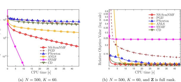
The convergence behaviors of different SymNMF solvers for the synthetic data sets are shown in Figure 2.1 and Figure 2.2. The results shown are averaged over 20 Monte Carlo (MC) trials with independently generated data. In Figure 2.1(a), the generatedZcan be exactly decomposed by SymNMF. It can be observed that NS-SymNMF and SNMF converge to the global optimal solution quickly, and SNMF is the fastest one among all compared algorithms. However, the case where the matrix can be exactly factorized is not common in most practical applications. Hence, we also consider the case where the matrix Z cannot be factorized exactly by a N ×K matrix.
(a)N = 500,K= 60. (b)N = 500,K= 60, andZis full rank. Figure 2.1 Data Set I: the convergence behaviors of different SymNMF solvers.
The results are shown in Figure2.1(b)and we use the relative objective value for comparison, i.e., kXXT
−Zk2F/kZk2F. We can observe that NS-SymNMF and CD can achieve a lower objective value than other methods. It is worth noting that there is a gap between SNMF and others, since the assumption of SNMF is not satisfied in this case.
(a) Objective Value (b) Optimality Gap
Figure 2.2 Data Set II: the convergence behaviors of different SymNMF solvers;N = 2000,
K = 4.
We also implement the algorithms on adjacency matrices (data set II), where the results are shown in Figure 2.2. The NS-SymNMF and SNMF algorithms converge very fast, but it can be observed that there is still a gap between SNMF and NS-SymNMF as shown in Figure 2.2(a).
We further show the convergence rates with respective to optimality gap versus CPU time in Figure 2.2(b). The optimality gap (2.14) measures the closeness between the generated sequence and the true stationary point. To get rid of the effect of the dimension ofZ, we usekX−proj+[X− ∇X(g(X,Y))]k∞ as the optimality gap. It is interesting to see the “swamp” effect (77), where the objective value generated by the CD algorithm remains almost constant during the time period from around 25s to 75s although actually the corresponding iterates do not converge, and then the objective value starts decreasing again.
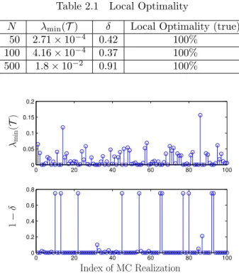
Table 2.1 Local Optimality
N λmin(T) δ Local Optimality (true)
50 2.71×10⁻⁴ 0.42 100% 100 4.16×10⁻⁴ 0.37 100% 500 1.8×10⁻² 0.91 100% 1 − δ λmin ( T ) Index of MC Realization
Figure 2.3 Checking local optimality condition, where N = 500.
2.4.3 Checking Global/Local Optimality
After the NS-SymNMF algorithm has converged, the local/global optimality can be checked according to Theorem 3 and Theorem 4. To find an appropriate δ that satisfying the condition where λmin(T) >0, we initialize δ as 1 and decrease it by 0.01 each time and check the minimum eigenvalue ofT. Here, we use data set II with the fixed ratio of the number of nodes within each
cluster (i.e., 3 : 5 : 8 : 4) and test on the different total numbers of nodes. The simulation results are shown in Table2.1 with 100 Monte Carlo trials, where the average value ofλmin(T) and δ are given. Further, the percentage of being able to find a validδ >0 that ensures λmin(T)>0 is listed as the last column. It can be observed that there always exists aδ such thatT is positive definite in all cases that we have tested. This indicates that (with high probability) the proposed algorithm converges to a locally optimal solution. In Figure 2.3, we provide the values of δ that make the correspondingλmin(T)>0 at each realization.
We also remark that in practice we stop the algorithm in finite steps, so only an approxi-mate KKT point will be obtained, and the degree of such approximation can be measured by the optimality gap defined in (2.14).
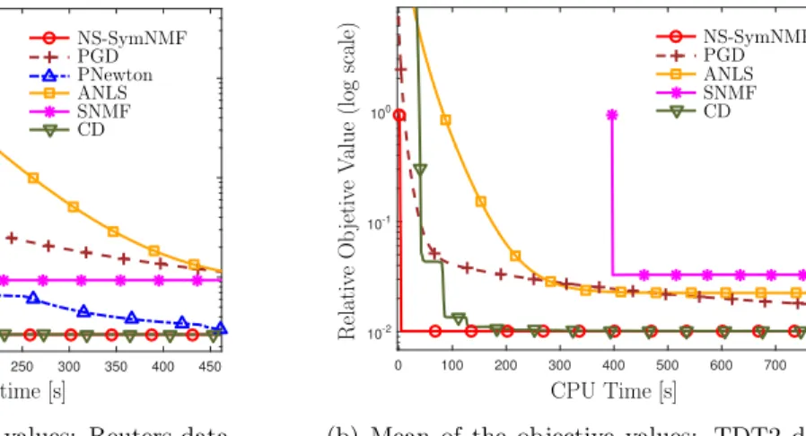
(a) Mean of the objective values: Reuters data set
(b) Mean of the objective values: TDT2 data set
Figure 2.4 The convergence behaviors of different SymNMF solvers for the dense similarity matrix.
2.4.4 Performance on Real Data
We also implement the algorithm on a few real data sets in clustering applications, which will be described in the next paragraphs.
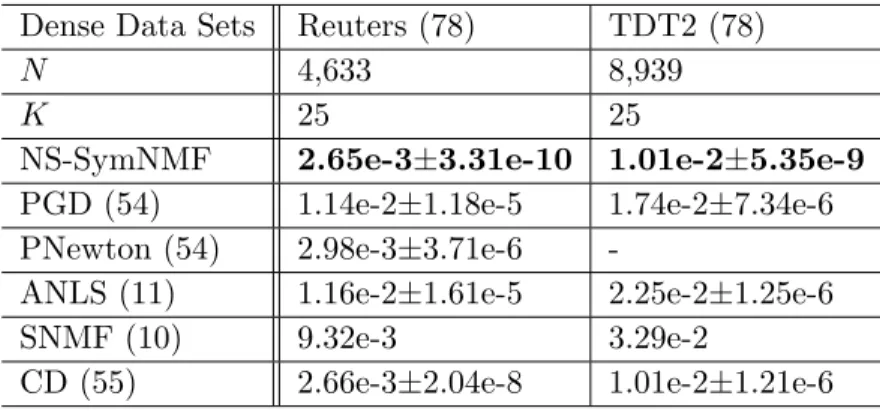
Table 2.2 Mean and Standard Deviation of kXXT −Zk2
F/kZk2F Obtained by the Final
Solution of Each Algorithm based on Random Initializations (dense similarity matrices)
Dense Data Sets Reuters (78) TDT2 (78)
N 4,633 8,939
K 25 25
NS-SymNMF 2.65e-3±3.31e-10 1.01e-2±5.35e-9 PGD (54) 1.14e-2±1.18e-5 1.74e-2±7.34e-6 PNewton (54) 2.98e-3±3.71e-6
-ANLS (11) 1.16e-2±1.61e-5 2.25e-2±1.25e-6
SNMF (10) 9.32e-3 3.29e-2
CD (55) 2.66e-3±2.04e-8 1.01e-2±1.21e-6
We generate the dense similarity matrices based on the two real data sets: Reuters-21578 (78) and TDT2 (78). We use the 10th subset of the processed Reuters-21578 data set, which includes N = 4,633 documents divided into K = 25 classes. The number of features is 18,933. Topic detection and tracking 2 (TDT2) corpus includes two newswires (APW and NYT), two radio programs (VOA and PRI) and two television programs (CNN and ABC). We use the 10th subset of the processed TDT2 data set with K = 25 classes which includes N = 8,939 documents and each of them has 36,771 features. We comment that the 10th TDT2 subset is the largest among the all TDT2 and Reuters subsets. Any other subset can be used equally well. The similarity matrix is constructed by the Gaussian function where the difference between two documents is measured by all features using the Euclidean distance (78).
The means and standard deviations of the objective values of the final solutions are shown in Table 2.2. Convergence results of the algorithms are shown in Figure 2.4. For the Reuters and TDT2 datasets, before SNMF completes the eigenvalue decomposition for the first iteration, CD and NS-SymNMF have already obtained very low objective values. Also, since the calculation of Hessian in PNewton is time consuming for large scale matrices, the result of PNewton is out of range in Figure2.4(b).
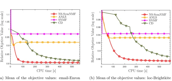
Sparse Similarity Matrix: We also generate multiple convergence curves for each algorithm with random initializations based on some sparse real data sets.
(a) Mean of the objective values: email-Enron data set
(b) Mean of the objective values: loc-Brightkite data set
Figure 2.5 The convergence behaviors of different SymNMF solvers for the sparse similar-ity matrix.
Table 2.3 Mean and Standard Deviation of kXXT
−Zk2F/kZk2F Obtained by the Final Solution of Each Algorithm based on Random Initializations (sparse similarity matrices)
Sparse Data Sets email-Enron (79) loc-Brightkite (80)
N 36,692 58,228
K 50 50
#nonzero 367,662 428,156
NS-SymNMF 8.05e-1±4.66e-4 8.75e-1±9.52e-4 ANLS (11) 9.18e-1±6.20e-3 9.33e-1±1.93e-3
SNMF (10) 9.69e-1 9.43e-1
CD (55) 8.13e-1±1.47e-3 8.84e-1±1.49e-3
Email-Enron network data set (79): Enron email corpus includes around half million emails. We use the relationships between two email addresses to construct the similarity matrix for decomposing. If an address i sent at least one email to address j, then we take Ai,j =Aj,i = 1. Otherwise, we
set Ai,j =Aj,i = 0.
Brightkite data set (80): Brightkite was a location-based social networking website. Users were able to share their current locations by checking-in. The friendships of the users were maintained by Brightkite. The way of constructing the similarity matrix is the same as the Enron email data set.
The means and standard deviations of the objective values of the final solutions are shown in Table 2.3. From the simulation results shown in Figure 2.5, it can be observed that the NS-SymNMF algorithm converges faster than CD, while SNMF and ANLS converge to some points where the relative objective values are higher than the one obtained by NS-SymNMF.
CHAPTER 3. STOCHASTIC SYMMETRIC NONNEGATIVE MATRIX FACTORIZATION
3.1 Introduction
In practical problems when there are multiple samples obtained, stochastic-type algorithm is the one of the most efficient options of handling stochastic optimization problems. Recently, the stochastic projected gradient descent (SPGD) methods are proposed for dealing with stochastic nonconvex problems (81; 82). However, there has been no convergence guarantee when directly applying SPGD to solve the stochastic SymNMF problem, since there is no global Lipschitz conti-nuity of the gradient of the objection function. Classical stochastic approximation methods can also be used, but without convergence and rate of convergence guarantees. Fast convergence rates of stochastic ADMM algorithms are presented recently (83; 84), however, these algorithms only work for stochastic convex optimization problems. In fact, none of the works has rigorous theoretical justification that they can be applied directly for SymNMF in the stochastic settings.
The most relevant algorithm that uses the nonconvex splitting method for solving SymNMF was proposed in (85), but the algorithm, called NS-SymNMF, only works for the case where the given data is deterministic. In this chapter, we consider the stochastic setting of matrix factorization that potentially make the SymNMF more practical. The proposed algorithm, named stochastic nonconvex splitting SymNMF (SNS-SymNMF), is a generalization of the previous NS-SymNMF algorithm, which is able to factorize the realizations of the random observation matrix in each iteration. Further, actually the convergence proof of NS-SymNMF does not apply to that of SNS-SymNMF, since the iterates are coupled with the random data matrices as the algorithm proceeds such that the boundness of the iterates is not clear if the convergence proof of NS-SymNMF was used.
In this work, SNS-SymNMF is proposed for problem (1.1), where the underlying distribution is unknown, but realizations of Zare available sequentially. The proposed algorithm belongs to the class of stochastic algorithms, because at each iteration only a few samples of the observation matrix are used. Based on different ways in which the samples are utilized, we analyze the performance of the algorithm in terms of its convergence rates to the set of stationary solutions of problem (1.1). The main contributions of this chapter are given below.
• The proposed algorithm possesses sublinear convergence rate guarantees. When an aggregate of the past samples is used (possibility with non-uniform weighting), the algorithm converges sublinearly to the stationary points of problem (1.1) in mean-square; when the instantaneous samples are used, the algorithm converges sublinearly to a neighborhood around the stationary solutions. To our best knowledge, this is the first stochastic algorithm that can possess a sublinear convergence rate for stochastic SymNMF.
• We demonstrate the performance of the proposed stochastic algorithm for clustering problems. It is shown that SNS-SymNMF is much faster compared with some existing algorithms for generic stochastic nonconvex optimization problems numerically. Further, due to the use of non-uniform aggregate sampling, the proposed algorithm is capable of tracking changes of the community structure.
3.2 Stochastic Nonconvex Splitting for SymNMF
3.2.1 Main Assumptions
The sequentially sampled data Zb(i) are assumed to be independent and identically distributed
(i.i.d.) realizations of the random matrixZ, whereidenotes the index of the sample. Rather than assuming the unbiased gradient and bounded variance of the stochastic gradient in most stochastic gradient methods (82), we only need to make assumptions on samples for SymNMF. Specifically, we assume the following.
Table 3.1 Rules of Aggregating Samples
Mini-batch Aggregate Weighted Aggregate
Z(1t)= 1 L PtL i=(t−1)L+1Zb (i) 1 Z (t) 1 = 1t Pt i=1Zb (i) 1 Z (t) 1 = t(t2+1) Pt i=1iZb (i) 1 Z(2t)= L1 PtL i=(t−1)L+1Zb (i) 2 Z (t) 2 = 1t Pt i=1Zb (i) 2 Z (t) 2 = t(t2+1) Pt i=1iZb (i) 2
• A2) Bounded variance: Tr[Var[Zb(i)]] =E[kZb(i)−Zk2F]≤σ2 ∀i;
• A3) Bounded magnitude: kZb(i)kF ≤ Z <∞ ∀i.
In practice, the magnitude of samples is finite, so A3 is valid (11; 82).
3.2.2 The Problem Formulation for Stochastic SymNMF
We start by considering the following reformulation of problem (1.1) to the following problem: min X,Y 1 2kXY T −EZ[Z]k2F (3.1) s.t. X=Y, Y≥0,kYik22 ≤τ, ∀ i whereZis a symmetric matrix; τ >0 is some given constant.
Under A1, it is easy to check that when τ is sufficiently large (with a lower bound dependent on Z), then problem (3.1) is equivalent to problem (1.1), in the sense that there is a one-to-one correspondence between the stationary points of problem (1.1) and (3.1), where the stationary condition of problem (1.1) is given by (27, Proposition 2.1.2)
X∗(X∗)T
−ZX∗,X−X∗≥0, ∀X∈ X.
whereX∗ denotes the stationary points. To be precise, we have the following result.
Lemma 3. Let Zi,k denote the(i, k)th entry of the matrix Z. Under A1 – A3, suppose τ > θk,∀k where θk, Zk,k+ q PN i=1Z2i,k 2 , (3.2)
then a point X∗ is a stationary point of problem (1.1) if and only if X∗ is a stationary point of problem (3.1).
Although the objective function does not have Lipschitz continuous gradient, Theorem 3 sug-gests that we can solve (1.1) within a compact set.
3.2.3 The Framework of SNS for SymNMF
To this end, let us construct the augmented Lagrangian for (2.3), given by L(X,Y;Λ) = 1 2kXY T −Z]k2F +hY−X,Λi+ρ 2kY−Xk 2 F (3.3)
where Λ ∈ RN×K is a matrix of dual variables (or Lagrange multipliers); h·i denotes the inner product operator;ρ >0 is a penalty parameter whose value will be determined later.
The proposed SNS-SymNMF algorithm alternates between the primal updates of variables X and Y, and the dual update for Λ. We split the data samples into two groups where Zb
(i)
1 is used for updating Y and Zb
(i)
2 is used forX, respectively. Our algorithm is also capable of dealing with a few different ways of aggregating the samples at each iteration:
1. A Mini-Batch ofL instantaneous samples are used; 2. An aggregate of the historical samples is used;
3. A special weighted aggregate of the historical samples is used.
See Table 3.1 for their mathematical descriptions. In the table, t denotes the tth iteration of the algorithm;Z(1t) and Z(2t) are the actual (aggregated) samples used in our algorithm.
In the following, we provide the main steps of the proposed algorithm. The implementation of each step will be provided shortly. At iterationt+ 1, we first compute the objective value evaluated at the previous sample, followed by the primal updates for Xand Y, finally the dual variable Λis updated. Specifically, β(t)=8 ρkX (t)(Y(t))T −Z(2t−1)k2F, (3.4a) Y(t+1)= arg min Y≥0,kYik22≤τ,∀i b LY(X(t),Y;Λ(t);Z(1t)), (3.4b) X(t+1)= arg min X LbX(X,Y (t+1);Λ(t);Z(t) 2 ), (3.4c) Λ(t+1)=Λ(t)+ρ(X(t+1)−Y(t+1)) (3.4d)
where we have defined b LY(X(t),Y;Λ(t);Z(1t)), 1 2kX (t)YT −Z(1t)k2F + ρ 2kX (t)−Y+Λ(t)/ρk2 F + β(t) 2 kY−Y (t)k2 F, b LX(X,Y(t+1);Λ(t);Z(2t)), 1 2kX(Y (t+1))T −Z(2t)k2F + ρ 2kX−Y (t+1)+Λ(t)/ρ k2F.
We remark that using independent samples for the X and Y update is critical in the convergence analysis of the algorithm.
3.2.4 Implementation of the SNS-SymNMF Algorithm
The implementation of SNS-SymNMF is shown in Algorithm1. The updates of variable Xand Y in each subproblem are the similar as the way in NS-SymNMF but with different strategy of using samples.
The SNS-SymNMF Algorithm. Leveraging the efficient calculation of Y(t+1) and X(t+1) (see (2.24) and (2.25)), we summarize the algorithm as shown in Algorithm1, whereT denotes the total number of iterations.
Algorithm 1 The SNS-SymNMF Algorithm 1: Input: Y(1),X(1),Λ(1), and ρ
2: fort= 1, . . . , T do
3: Update β(t) according to (3.4a) 4: Select data using Table 3.1 5: Update Y(t+1) by solving (3.4b) 6: Update X(t+1) by solving (3.4c) 7: Update Λ(t+1) using (3.4d) 8: end for
9: Output: IterateY(r) chosen uniformly random from {Y(t)}T t=1.
3.3 Convergence Analysis
The convergence analysis is built upon a series of lemmas (shown in the supplemental materials of (86)), which characterize the relationship among the augmented Lagrangian, the primal/dual variables as well as the random samples.
We also remark the convergence proof of SNS-SymNMF is different from the work in the previous chapter. Here we start from the proof of the boundness of the X-iterate, then the convergence of the algorithm to stationary points can be characterized.
Theoretical Results. First, when a mini-batch of samples are used at each iteration, we have the following result.
Theorem 5. Suppose A1 – A3 hold true. Then the iterates generated by the SNS-SymNMF algo-rithm with Mini-Batch samples satisfy the following relation
E[PMini-Batch(X(r),Y(r),Λ(r))]≤ 1 TC(U+ σ2 L) + Wσ2 L
where C,U,W are some constants.
Theorem 5 says that using the Mini-Batch samples the SNS-SymNMF algorithm converges sublinearly to a ball of size Wσ2/L around the stationary points of problem (2.3). Further, the radius of the ball can be reduced when increasing the number of samples L.
Second, if all the past samples are averaged using the same weight, then the algorithm can converge to the stationary points of the stochastic SymNMF problem.
Theorem 6. Suppose A1 – A3 hold true and the following is satisfied
ρ >8N Kτ2. (3.5)
Then the following statements are true for SNS-SymNMF with averaged samples: 1. The equality constraint is satisfied in the limit, i.e.,
lim
t→∞E[kX (t)
−Y(t)k2F]→0.
2. The sequence{X(t),Y(t),Λ(t)}is bounded, and every limit point of the sequence is a stationary point of problem (3.1).
Theorem 7. Suppose A1 – A3 hold true. Then the iterates generated by the SNS-SymNMF algo-rithm with aggregate samples satisfy the following relation
E[Paggregate(X(r),Y(r),Λ(r))]≤ CS
+Cσ2+Kσ2 T
where C,S,K are some constants.
Theorem 6 and Theorem 7 show that the stochastic SymNMF can converge to a stationary point of (3.1) in mean-square, and in a sublinear manner. Then, we have the following corollary directly.
Corollary 2. Suppose A1 – A3 hold true. Then the iterates generated by the SNS-SymNMF algorithm with weighted aggregate samples satisfy the following relation
E[Pweighted(X(r),Y(r),Λ(r))]≤ CS
+Cσ2+K0σ2 T
where K0 ≥ K.
Remark 1. Those constants, such asC,U,W,S,K, mentioned in the theorems are only depen-dent on the initialization of the algorithm and parameters of given problems, such as N, K, τ,Z. The explicit expressions of the constants can be found in the supplemental materials of (86).
It is worth noting that when σ2 = 0, our convergence analysis of the SNS-SymNMF algorithm still holds true for the deterministic case (85).
We also remark that given a required error, when the dimension of the problems increases, the stochastic algorithms need a more total number of iterations to achieve this error.
3.4 Numerical Results
3.4.1 Synthetic Data Set
Data Set Description. We use a similar random graph as adopted in (14) for spectral clustering. The graph is generated as follows. For each time slot, data points {xi} ∈ R, i = 1, . . . , N, are
are 12, 24, 48 and 36. Within each cluster, data points follow an i.i.d. Gaussian distribution. The means of the random variables in these 4 clusters are 2,4,6,8, respectively, and the variance is 0.5 for all distributions. Then, construct the similarity matrix Zb
(i)
1 ∈ RN×N (or Zb
(i)
2 ), whose (i, j)th entry is determined by the Gaussian function exp(−(xi −xj)2/(2σ2)) where σ2 = 0.5.
Finally, we repeat the process mentioned above to generate a series of adjacency matrices for the community detection problem. The mean of the adjacency matrix represents the ground truth of the connections among the nodes and variance measures the uncertainty of each sample. Based on this model, we know that the weights between two points which belong to the same cluster are very likely higher than the weights between two points which belong to different clusters.
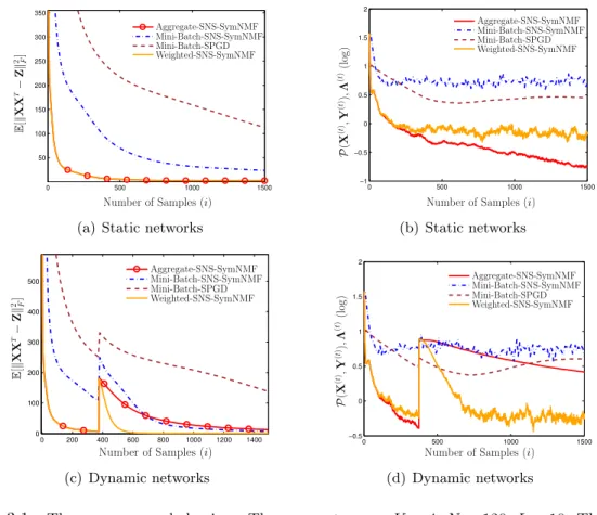
Number of Samples (i) E [ XX T− Z 2]F Aggregate-SNS-SymNMF Mini-Batch-SNS-SymNMF Mini-Batch-SPGD Weighted-SNS-SymNMF
(a) Static networks
Number of Samples (i) P ( X ( t ),Y ( t )), Λ ( t )( log ) Aggregate-SNS-SymNMF Mini-Batch-SNS-SymNMF Mini-Batch-SPGD Weighted-SNS-SymNMF (b) Static networks Number of Samples (i) E [ XX T− Z 2]F Aggregate-SNS-SymNMF Mini-Batch-SNS-SymNMF Mini-Batch-SPGD Weighted-SNS-SymNMF (c) Dynamic networks Number of Samples (i) P ( X ( t ),Y ( t )), Λ ( t )( log ) Aggregate-SNS-SymNMF Mini-Batch-SNS-SymNMF Mini-Batch-SPGD Weighted-SNS-SymNMF (d) Dynamic networks
Figure 3.1 The convergence behaviors. The parameters areK= 4; N= 120; L= 10. Thex-axis represents the total number of observed samples.
Algorithms Comparison. Each point in Figure3.1is an average of 20 independent Monte Carlo (MC) trials. All algorithms are started with the same initial point each time, and the entries of
![Figure 4.1 Contour of the objective values and the trajectory (pink color) of PA-GD started near strict saddle point [0, 0]](https://thumb-us.123doks.com/thumbv2/123dok_us/8991362.2797020/55.918.298.621.157.427/figure-contour-objective-values-trajectory-started-strict-saddle.webp)