Laurens Vanderstraeten,1,∗ Jutho Haegeman,1 and Frank Verstraete1, 2
1
Department of Physics and Astronomy, University of Ghent, Krijgslaan 281, 9000 Gent, Belgium 2
Vienna Center for Quantum Science and Technology, Faculty of Physics, University of Vienna, Boltzmanngasse 5, 1090 Vienna, Austria
We develop and benchmark a technique for simulating excitation spectra of generic two-dimensional quantum lattice systems using the framework of projected entangled-pair states (PEPS). The technique relies on a variational ansatz for capturing quasiparticle excitations on top of a PEPS ground state. Our method perfectly captures the quasiparticle dispersion relation of the square-lattice transverse-field Ising model, and reproduces the spin-wave velocity and the spin-wave anomaly in the square-lattice Heisenberg model with high precision.
Quantum phases of matter are commonly char-acterized by the order of the ground states that are realized in many-body systems at zero temper-ature. Yet, the most interesting manifestations, both from the theoretical and the experimental perspective, of a given quantum phase are more related to the low-energy excitations on top of the ground state. In the case of strongly-correlated quantum phases these excitations typically have a collective nature, in the sense that they cannot be adiabatically connected to the excitations of a free system. Therefore, perturbative expansions or mean-field approximations do not allow for an ac-curate description, and more advanced conceptual and numerical tools have to be devised to under-stand their properties. This is especially true for one- and two-dimensional quantum systems, where strong quantum correlations often lead to collec-tive excitations with fractionalized quantum num-bers and anyonic statistics.
Tensor networks have emerged as a natural lan-guage for describing quantum phases of matter. It has been realized that these phases are character-ized by the entanglement structure of their low-energy states, and that this structure can be cap-tured by the class of tensor-network states1,2. In one dimension, this yields the well-kown class of matrix product states3 (MPS) describing ground
states of generic spin chains, as well as a powerful formalism for capturing quasiparticle excitations on top of these strongly-correlated background states4. In this formalism, elementary excitations of the fully-interacting quantum Hamiltonian5
are naturally interpreted as interacting particles (including magnons, triplons spinons, chargeons, holons, etc.6) and a two-particle S matrix can be
defined and computed7. For two-dimensional sys-tems, the class of projected entangled-pair states (PEPS)8 provides the correct parametrization of
ground states, and PEPS constructions for describ-ing quasiparticles such as spinons9and anyons10,11
have been proposed.
Yet, these constructions of quasiparticles against a PEPS background have been used numerically on fine-tuned wavefunctions only12,13, and have
not been applied variationally to characterize the spectrum of a given model Hamiltonian. In-deed, PEPS simulations have been restricted to the study of ground-state properties of ordered quan-tum magnets14–17, (chiral) spin liquids18–20, and strongly-correlated electrons16,21, but, thanks to considerable progress in MPS techniques22,23, in
recent years a second generation of PEPS algo-rithms has started to form. The variational op-timization of PEPS ground-state approximations has been made possible24,25, which allows to obtain higher accuracy on ground-state energies and or-der parameters. This, in turn, has made it possible to develop accurate extrapolation techniques26,27.
In addition, quantities such as momentum-resolved structure factors or the energy variance can be computed with high accuracy25.
These techniques now make it possible to go be-yond ground-state properties, and to simulate the excitation spectrum of a given Hamiltonian with PEPS. A first step was taken in Ref. 22, but limited to the special case of frustration-free Hamiltonians. In this work, we generalize this framework to sim-ulate the excitation spectrum of generic Hamilto-nians on two-dimensional lattices in the thermody-namic limit directly, and benchmark this method on the transverse-field Ising model and the square-lattice Heisenberg model.
The algorithm— The PEPS simulation of the ex-citation spectrum of a given model Hamiltonian H =P
ihi consists of two steps. In a first step, we find an optimal approximation for the model’s ground state in terms of a PEPS tensor A. The ground-state wavefunction can be written down as
|Ψ(A)i= , (1)
which represents the contraction of an infinite
work of the same five-leg tensor A, Asu,r,l,d= r d l u s . (2)
The index s corresponds to the physical spin at each site, and the four virtual legs carry the corre-lations through the system; the dimension of these virtual legs is the so-called bond dimension D of the PEPS, and serves as a control parameter in all PEPS simulations. Different algorithms were de-veloped for finding an optimal PEPS representa-tion with a given bond dimension in a variarepresenta-tional way. In this work, we have used gradient-search methods25 that variationally optimize the energy
density directly in the thermodynamic limit. In a next step, we build elementary excitations on top of this ground state. For these excitations we consider the variational ansatz
|Φ~q(B)i= X
~ m∈L
ei~q·m~ m~ . (3)
Here a new tensor B is introduced at one site in the network (the round tensor), and a superposi-tion is taken with momentum ~q= (qx, qy), which, because we work directly in the thermodynamic limit, ranges through the full Brillouin zone. Be-cause the perturbation also acts on the virtual degrees of freedom in the PEPS, it can create a dressed object against a correlated background; in that sense, it can be interpreted as the PEPS gen-eralization of the Feynman-Bijl ansatz28or single-mode approximation29.
In the ansatz wavefunction all variational free-dom is contained within the tensor B. Moreover, as the wavefunction is clearly linear in the tensor B, the ansatz defines a linear subspace. The inner product within this subspace is found by comput-ing the overlap between two states,
hΦ~q0(B0)|Φ~q(B)i
= 4π2δ(2)(~q−~q0)(B0)†N~qB, (4) where bold symbols denote the vectorized versions of the corresponding tensors. Up to a δ function normalization for the momenta, the inner product is determined by the effective norm matrix N~q. As was shown in Ref. 22, some choices for the ten-sor B give rise to a zero state in Eq. (3). Also, we want to confine our variational space to states that are locally orthogonal to the ground state. In the end, these restrictions lead to a basisP for the reduced subspace such that the projected norm matrixP†N~qP is full rank.
Evaluating the overlap between two excited-state wavefunctions [Eq. (4)], and a fortiori the computation of the effective norm matrix, requires an involved contraction. Indeed, this overlap re-duces to a sum over all relative positions between the tensor B in the ket vector and the tensorB0 in the bra. All these terms have the form of a two-point function
, (5)
where we have taken a top view of the double-layer (bra and ket) tensor-network diagram, the simple circle represents the contraction of a ground-state tensor A and its conjugate, and the crosses de-note where the B tensor in the ket layer and the
¯
B0 tensor in the bra layer are situated. It should be clear that these terms are determined by the correlations in the ground state, and in Ref. 22 a contraction scheme was developed that provides an effective channel environment for reducing the above diagram to an essentially one-dimensional contraction. In fact, these channel environments enable the full summation of all relative positions of the tensors in an efficient way, and, therefore, allow for an evaluation of N~q. The accuracy of this channel construction is controlled by the en-vironment bond dimensionχ.
The variational optimization of the B tensor now requires minimizing the excitation energy. Be-cause of the linearity of the variational subspace, this amounts to solving the generalized eigenvalue problem P†H~qP x~q=ω(~q) P†N~qP x~q, (6) for the smallest-real eigenvalue. Here we have in-troduced the effective energy matrix
hΦ~q0(B0)|H˜|Φ~q(B)i
= 4π2δ(2)(~q−~q0)(B0)†H~qB. (7) The eigenvalueω(~q) is the approximate excitation energy at momentum~q, whereas the state|Φq~(B)i with B = P x~q, approximates the excited-state wavefunction. The renormalized Hamiltonian ˜H is obtained by subtracting the extensive ground-state energy, i.e. H˜ =P
i(hi− hhii0), such that
we find non-extensive excitation energies above the ground state.
The evaluation of the matrix elements of H~q [Eq. (7)] involves the summation of three-point functions, but can, through a strategic position-ing of channel environments, again be reduced to
FIG. 1. The quasiparticle dispersion for the square-lattice transverse-field Ising model at λ = 2.5 (blue),
λ= 2.7 (red) andλ= 2.9 (yellow), as computed from PEPS with bond dimension D = 3 and environment bond dimension χ = 50. The blue dots are series-expansion data points extracted from Ref. 30.
a number of one-dimensional contractions. We re-fer to the supplemental material for a full exposi-tion of all tensor-network diagrams. The hardest diagrams, and therefore the computational com-plexity of implementing the generalized eigenvalue problem [Eq. (6)], scales asO(D6χ3+D8χ2). Benchmark results— As a first example we test our method on the transverse-field Ising model, defined by the Hamiltonian Hising=− X hiji SizSjz+λX i Six. (8)
This model exhibits a quantum phase transition atλc≈3.044 from a symmetry-broken phase (λ < λc) to a polarized phase (λ > λc). In Ref. 25 it was shown that the ground state of this model can be accurately approximated as a PEPS across the phase transition.
We can now build excitations on top of this ground state, and compute the quasiparticle spec-trum. In Fig. 1 our results are plotted for the quasiparticle dispersion relation at three different values of the field; for one value of the field we com-pare with results from series expansions30. The dispersion clearly reaches a minimum at momen-tum~q= (0,0), yielding the value of the gap. The phase transition is signalled by the vanishing of the excitation gap; in fact, close to the phase transi-tion, the gap should obey a scaling relation with a critical exponentν ≈0.623030. In Fig. 2 we have plotted the gap as a function of the field, show-ing that the power-law scalshow-ing is reproduced over a large region. We find estimates for the critical exponentνand the critical fieldλwithin a percent precision.
A more challenging and interesting benchmark
FIG. 2. The gap of the Ising model as a function of the field λ, with a fit ∆ ∝ |λ−λc|ν
; we find λc ≈3.066 andν≈0.627. We have usedD= 3 andχ= 50.
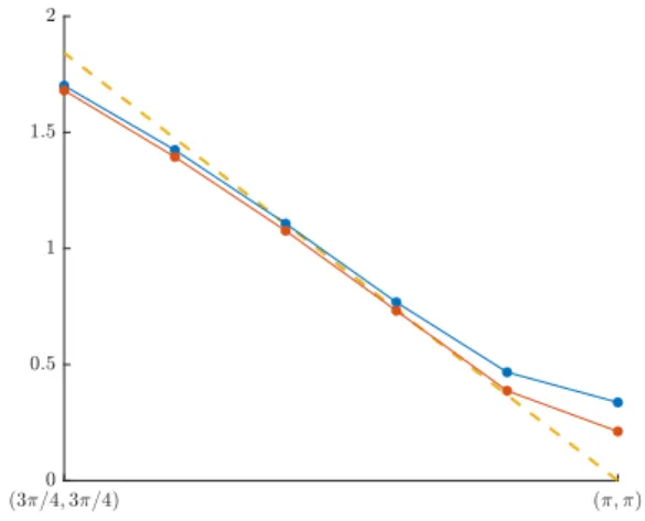
FIG. 3. The dispersion relation of the Heisenberg model approaching the gapless point (π,0) with bond dimensionD= 3 (blue) andD= 4 (red) and environ-ment bond dimension up toχ= 100, as compared to the linear dispersion relation withvs≈1.6584731 (yel-low). Clearly, the finite bond dimension of the PEPS induces an artificial gap, which grows smaller asD in-creases. If we estimate the spin-wave velocity as the slope at the inflection point in the D = 4 curve, we findvs≈1.638.
is provided by the Heisenberg model, defined by the Hamiltonian
Hheis= X
hiji
SixSxj −SiySyj −SizSjz. (9)
Here we have introduced the minus signs through a sublattice rotation of the original Heisenberg Hamiltonian, such that the staggered magnetiza-tion is mapped to a uniform one. Therefore, we can approximate the ground state as a uniform PEPS with a one-site unit cell25.
Since the ground state breaks a continuous sym-metry, the spectrum exhibits a gapless Goldstone mode. The slope of the dispersion relation around
(π/2, π/2) (π,0) QMC34 2.4085 2.13 pCUT35 2.375 2.2 ED36 2.4144 2.2281 DMRG 2.40 2.06-2.07 D= 4 2.39 2.19
TABLE I. The estimates for the excitation energies at wavevectors ~q = (π/2, π/2) and ~q = (π,0) as com-puted by some state-of-the-art numerical techniques, and compared to our PEPS result atD= 4.
the gapless point or spin-wave velocityvsis a cru-cial quantity in any low-energy field theory for this model32,33 and is directly accessible in e.g.
neutron-scattering experiments. In Fig. 3 we have plotted the dispersion relation in a small portion of the Brillouin zone where the gap is expected to close. Because the finite bond dimension induces a finite correlation length in the ground state26,27,
the dispersion relation exhibits an artificial gap. This effect is clearly seen in our results, but is di-minished as the bond dimension increases. Besides this effect, we reproduce the linear dispersion and we obtain an estimate for the spin-wave velocity that is close to the Monte-Carlo estimate.
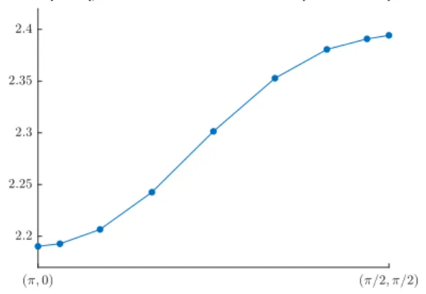
A more interesting feature of the spectrum is the shape of the dispersion relation at higher en-ergies. Linear spin-wave theory predicts that the excitation gap is constant on the line between the wavevectors (π,0) and (π/2, π/2), but vari-ous numerical approaches34–40 and experimental measurements41 have shown that the excitation
energy is suppressed at (π,0) and elevated at (π/2, π/2) as compared to the spin-wave result. The physical origin of this discrepancy has been ar-gued to follow from spinon deconfinement around the wavevector (π,0). In Fig. 4 we have plotted our results for the dispersion in this region, show-ing a significant dip in the dispersion. In Table I we compare our excitation energies to some other numerical results available in the literature. As to the physical origin of the spin-wave anomaly, we should note that the fact that our quasiparti-cle ansatz can accurately reproduce the excitation energy at (π,0) suggests that this state is quite far from a deconfined two-spinon state.
Outlook— In this work we have presented a PEPS method for simulating excitation spectra of generic Hamiltonians in two dimensions, and have bench-marked the method on the Ising and Heisenberg models on the square lattice. The method can be readily extended to other lattice structures and PEPS ground states with larger unit cells. Al-though we have applied it to models that exhibit a local order parameter, our method can be
ap-plied equally well to more exotic quantum phases
FIG. 4. The dispersion relation of the Heisenberg model between the points (π,0) and (π/2, π/2), com-puted with PEPS atD= 4 andχ= 100.
such as spin liquids and systems with topological order. In particular, the PEPS framework allows to directly target the fractionalized quasiparticles in these systems.
On the technical side many improvements of the method can be made. The conditioning of the gen-eralized eigenvalue problem is, due to small eigen-values in the effective norm matrixN~q, a source of large errors, and, therefore, a well-chosen precondi-tioner is required. Also, the implementation ofH~q requires the contraction of a large number of differ-ent diagrams and is therefore computationally de-manding; better contraction schemes can speed up the simulations considerably. This, in turn, would make higher values of the PEPS bond dimension feasible, which would enable the use of extrapola-tion techniques for e.g. the excitaextrapola-tion energies. Fi-nally, the exploitation of symmetries in the PEPS representation of the ground state as well as the quasiparticle excitations will lead to much more efficient simulations.
In the context of matrix product states, this method of describing excitation spectra falls within the set of so-called tangent-space methods42. This numerical framework starts from the idea that the class of uniform MPS constitutes a manifold that describes ground states of spin chains, but real-izes that the low-energy dynamics around such a ground state is contained within the tangent space on this manifold. In this work, we show that these tangent-space methods can also be applied to the PEPS manifold, and we expect that this will prove extremely useful in the simulation of the low-energy dynamics of two-dimensional quantum matter.
Acknowledgements— The authors would like to thank Kai Schmidt and Ruben Verresen for sharing their data. This work is supported by the Research Foundation Flanders, ERC grants QUTE (647905) and ERQUAF (715861), and the EU grant SIQS.
∗
F. Verstraete, V. Murg, and J. I. Cirac, “Ma-trix product states, projected entangled pair states, and variational renormalization group methods for quantum spin systems,” Advances in Physics 57, 143–224 (2008).
2 R. Or´us, “A practical introduction to tensor net-works: Matrix product states and projected entan-gled pair states,” Annals of Physics 349, 117–158 (2014).
3
U. Schollw¨ock, “The density-matrix renormaliza-tion group in the age of matrix product states,” Annals of Physics326, 96–192 (2011).
4 J. Haegeman, B. Pirvu, D. J. Weir, J. I. Cirac, T. J. Osborne, H. Verschelde, and F. Verstraete, “Vari-ational matrix product ansatz for dispersion rela-tions,” Physical Review B85, 100408 (2012). 5
J. Haegeman, S. Michalakis, B. Nachtergaele, T. J. Osborne, N. Schuch, and F. Verstraete, “Elemen-tary excitations in gapped quantum spin systems,” Physical Review Letters111, 080401 (2013). 6
V. Zauner-Stauber, L. Vanderstraeten, J. Haege-man, I. P. McCulloch, and F. Verstraete, “Topolog-ical nature of spinons and holons: Elementary exci-tations from matrix product states with conserved symmetries,” Physical Review B97, 235155 (2018). 7 L. Vanderstraeten, F. Verstraete, and J. Haege-man, “Scattering particles in quantum spin chains,” Physical Review B92, 125136 (2015).
8 F. Verstraete and J. I. Cirac, “Renormalization algorithms for Quantum-Many Body Systems in two and higher dimensions,” arXiv (2004), cond-mat/0407066.
9
D. Poilblanc and N. Schuch, “Simplexz2spin liquids on the kagome lattice with projected entangled pair states: Spinon and vison coherence lengths, topo-logical entropy, and gapless edge modes,” Physical Review B87, 140407 (2013).
10 N. Schuch, J. I. Cirac, and D. P´erez-Garc´ıa, “Peps as ground states: Degeneracy and topology,” An-nals of Physics325, 2153 – 2192 (2010).
11
N. Bultinck, M. Marin, D.J. Williamson, M. B. S¸ahino˘glu, J. Haegeman, and F. Verstraete, “Anyons and matrix product operator algebras,” Annals of Physics378, 183 – 233 (2017).
12 J. Haegeman, V. Zauner, N. Schuch, and F. Ver-straete, “Shadows of anyons and the entanglement structure of topological phases,” Nature Communi-cations6, 8284 (2015).
13
M. Iqbal, K. Duivenvoorden, and N. Schuch, “Study of anyon condensation and topological phase transitions from a z4 topological phase using the projected entangled pair states approach,” Physical Review B97, 195124 (2018).
14
P. Corboz, A. M. L¨auchli, K. Penc, M. Troyer, and F. Mila, “Simultaneous dimerization and su(4) sym-metry breaking of 4-color fermions on the square lat-tice,” Physical Review Letters107, 215301 (2011). 15 P. Corboz and F. Mila, “Crystals of bound states in the magnetization plateaus of the shastry-sutherland model,” Physical Review Letters 112,
147203 (2014). 16
P. Corboz, T. M. Rice, and M. Troyer, “Competing states in thet-jmodel: Uniformd-wave state versus stripe state,” Physical Review Letters113, 046402 (2014).
17
I. Niesen and P. Corboz, “Emergent haldane phase in thes= 1 bilinear-biquadratic heisenberg model on the square lattice,” Physical Review B 95, 180404 (2017).
18 H. J. Liao, Z. Y. Xie, J. Chen, Z. Y. Liu, H. D. Xie, R. Z. Huang, B. Normand, and T. Xiang, “Gapless spin-liquid ground state in thes= 1/2 kagome anti-ferromagnet,” Physical Review Letters118, 137202 (2017).
19
D. Poilblanc and M. Mambrini, “Quantum criti-cal phase with infinite projected entangled paired states,” Physical Review B96, 014414 (2017). 20
J.-Y. Chen, L. Vanderstraeten, S. Capponi, and D. Poilblanc, “Non-abelian chiral spin liquid in a quantum antiferromagnet revealed by an ipeps study,” arXiv (2018), 1807.04385.
21
B.-X. Zheng, C.-M. Chung, P. Corboz, G. Ehlers, M.-P. Qin, R. M. Noack, H. Shi, S. R. White, S. Zhang, and G. K.-L. Chan, “Stripe order in the underdoped region of the two-dimensional hubbard model,” Science358, 1155–1160 (2017).
22 L. Vanderstraeten, M. Mari¨en, F. Verstraete, and J. Haegeman, “Excitations and the tangent space of projected entangled-pair states,” Physical Review B 92, 201111 (2015).
23
M.T. Fishman, L. Vanderstraeten, V. Zauner-Stauber, J. Haegeman, and F. Verstraete, “Faster methods for contracting infinite 2d tensor net-works,” arXiv (2017), 1711.05881.
24
P. Corboz, “Variational optimization with infinite projected entangled-pair states,” Physical Review B94, 035133 (2016).
25
L. Vanderstraeten, J. Haegeman, P. Corboz, and F. Verstraete, “Gradient methods for variational optimization of projected entangled-pair states,” Physical Review B94, 155123 (2016).
26
M. Rader and A. M. L¨auchli, “Finite correlation length scaling in lorentz-invariant gapless ipeps wave functions,” Physical Review X 8, 031030 (2018).
27 P. Corboz, P. Czarnik, G. Kapteijns, and L. Tagli-acozzo, “Finite correlation length scaling with infi-nite projected entangled-pair states,” Physical Re-view X8, 031031 (2018).
28
R. P. Feynman, “Atomic Theory of the Two-Fluid Model of Liquid Helium,” Physical Review94, 262– 277 (1954).
29 D. P. Arovas, A. Auerbach, and F. D. M. Hal-dane, “Extended Heisenberg models of antiferro-magnetism: Analogies to the fractional quantum Hall effect,” Physical Review Letters60, 531–534 (1988).
30
J. Oitmaa, C. Hamer, and W. Zheng,Series Expan-sion Methods for Strongly Interacting Lattice Models (Cambridge University Press, 2006).
31
of excitations in ordered, disordered, and critical antiferromagnets,” Physical Review B 92, 195145 (2015).
32 S. Chakravarty, B. I. Halperin, and D. R. Nel-son, “Two-dimensional quantum heisenberg antifer-romagnet at low temperatures,” Physical Review B 39, 2344–2371 (1989).
33
A. V. Chubukov, S. Sachdev, and J. Ye, “Theory of two-dimensional quantum heisenberg antiferromag-nets with a nearly critical ground state,” Physical Review B49, 11919–11961 (1994).
34
A. W. Sandvik and R. R. P. Singh, “High-energy magnon dispersion and multimagnon continuum in the two-dimensional heisenberg antiferromagnet,” Physical Review Letters86, 528–531 (2001). 35
M. Powalski, G. S. Uhrig, and K. P. Schmidt, “Ro-ton minimum as a fingerprint of magnon-higgs scat-tering in ordered quantum antiferromagnets,” Phys-ical Review Letters115, 207202 (2015).
36 A. L¨uscher and A. M. L¨auchli, “Exact diagonaliza-tion study of the antiferromagnetic spin-1
2 heisen-berg model on the square lattice in a magnetic field,” Physical Review B79, 195102 (2009). 37
R. R. P. Singh and M. P. Gelfand, “Spin-wave exci-tation spectra and spectral weights in square lattice
antiferromagnets,” Physical Review B52, R15695– R15698 (1995).
38
W. Zheng, J. Oitmaa, and C. J. Hamer, “Series studies of the spin-1
2 heisenberg antiferromagnet at
t = 0: Magnon dispersion and structure factors,” Physical Review B71, 184440 (2005).
39 H. Shao, Y. Q. Qin, S. Capponi, S. Chesi, Z. Y. Meng, and A. W. Sandvik, “Nearly deconfined spinon excitations in the square-lattice spin-1/2 heisenberg antiferromagnet,” Physical Review X7, 041072 (2017).
40
M. Powalski, K. P. Schmidt, and G. S. Uhrig, “Mu-tually attracting spin waves in the square-lattice quantum antiferromagnet,” SciPost Phys. 4, 001 (2018).
41
B. Dalla Piazza, M. Mourigal, N. B. Christensen, G. J. Nilsen, P. Tregenna-Piggott, T. G. Per-ring, M. Enderle, D. F. McMorrow, D. A. Ivanov, and H. M. Rønnow, “Fractional excitations in the square-lattice quantum antiferromagnet,” Nature Physics11, 62 (2015).
42
L. Vanderstraeten, J. Haegeman, and F. Verstraete, “Tangent-space methods for uniform matrix prod-uct states,” in preparation.
APPENDIX: IMPLEMENTING THE PEPS QUASIPARTICLE ANSATZ
In this appendix we provide the details for implementing and optimizing the PEPS excitation ansatz. We work on the square lattice for which the ground state can be represented as a translation- and rotation-invariant PEPS, and we take the case of a translation invariant Hamiltonian with terms acting on a plaquette of four sites. We assume that we have an optimized ground-state approximation, for the details of how to variationally optimize the ground-state PEPS tensor we refer to Ref. 25. In order to make this appendix self-contained, we recapitulate the construction of effective channel environments22
in a first section, and then explain the excitation ansatz in detail.
1. Uniform PEPS and effective environments We assume that the ground state of the Hamiltonian is given by a PEPS,
|Ψ(A)i= (1)
where the wiggly lines correspond to the physical degrees of freedom. The tensors appearing in the PEPS are all copies of the same tensorA,
Asu,r,d,l= r
d l
u s
, (2)
and we assume that the tensor is rotation invariant,
Asu,r,d,l=Asl,u,r,d=Asd,l,u,r =Asr,d,l,u, (3) so that the state |Ψ(A)i is too (everything below can be readily generalized to non-rotation invariant case).
The norm of a PEPS can be represented as
hΨ(A)|Ψ(A)i= , (4)
where the round tensor represents the contraction of anA tensor with its complex conjugate along the physical dimension, and we have grouped two legs into one in each direction,
{r, r0} {d, d0} {l, l0} {u, u0} =X s,s0 δs,s0Asu,r,d,lA¯s 0 u0,r0,d0,l0. (5)
The contraction of this infinite tensor network is performed by finding the fixed point of the linear transfer matrix in the form of an MPS on the virtual level. This MPS obeys the fixed-point equation
∝ . (6)
Here, the MPS is represented by a triple of tensors{Al, Ar, C} which obey the conditions
Al C = C Ar , (7) and Al ¯ Al = , Ar ¯ Ar = . (8)
The ‘norm per site’f =−1
N log(hΨ(A)|Ψ(A)i) corresponding to the PEPS is then defined as
f =−logλ, (9)
where λis given as the leading eigenvalue of the following eigenvalue equations
Al ¯ Al Gl =λGl , Ar ¯ Ar Gr =λ Gr (10)
The corresponding eigenvectors Gl andGrare normalized such that
1 λ Mc ¯ Mc Gl Gr = Gl Gr ¯ C C = 1 (11)
We can now rescale the PEPS tensorA as
A→A/√λ, (12)
such that we havef = 0, and all PEPS expectation values are well-defined in the thermodynamic limit. In addition, we define a corner tensorS which is the leading eigenvector of the equation
Ar Ar Ar Al Al Al S ¯ Ar ¯ Al A¯l A¯l A¯l ¯ Ar ¯ Ar ¯ Ar ∝ S , (13)
which can be simplified to S ¯ Al ¯ Ar Gl Gr ∝ S . (14)
In order to compute expectation values we find four environments {Ml, Mr, C}i which we use to determine the contraction of the norm of the PEPS as
Ml Ml Mc Mr Mr
Mr Mr Mc Ml Ml
. (15)
The MPS tensors {Ml, Mr} are given by {Al, Ar} but normalized such that the following eigenvalue equation has leading eigenvalueµ= 1:
Ml
Mr
ρ =µ ρ . (16)
The PEPS can now be fully normalized by rescaling the corresponding eigenvectorρsuch that
hΨ(A)|Ψ(A)i= ρ ρ
C
C
= 1. (17)
We also define the fixed point in the other direction ˜ρas
Ml
Mr
˜
ρ =µ ρ˜ (18)
and normalize it such that
ρ ρ˜ = 1. (19)
The norm of the PEPS is then also given by
hΨ(A)|Ψ(A)i=
Ml
Mr
ρ ρ˜ = 1 (20)
We now define the corner environment
Mr
Mr
Mr
Ml Ml Ml S
where the corner matrix S is normalized such that, again, the norm of the PEPS is one: hΨ(A)|Ψ(A)i= Mr Mr Mr Ml Ml Ml S S Mr Mr Mr Ml Ml Ml Mr Mr Mr Ml Ml Ml Ml Ml Ml Mr Mr Mr S S = ρ ρ ρ ρ = 1. (22)
We also define two-site channel fixed points as ρ
Mr Ml =µ
ρ
. (23)
Because of the redefinition ofMlandMr, the eigenvalueµshould be (approximately) one. We also define the other fixed point,
Mr Ml ˜ ρ =µ ˜ ρ . (24)
Note that we overload the symbols for tensors, where its definition depends on the number of legs it has. The energy density expectation value is given by the two equivalent diagrams
e= ρ ρ Mr ρ Mr Mr Mr ρ = ρ ρ ρ ρ ρ , (25)
where we have introduced the dashed lines to indicate the four sites on which the Hamiltonian plaquette operator acts.
2. The ansatz wavefunction We use the following ansatz for an excitation with momentum (qx, qy)
|Φ~q(B)i= X k,l eiqxkeiqyl (k, l) (26)
where the round tensor denotes a new tensor B, Bu,r,d,ls = u r d l s , (27)
containing all variational degrees of freedom in the excited state. The overlap between the ground state and an excited state can be easily computed. We first introduce the following notation for a double-layer tensor containing aB tensor in the ket-level,
{u, u0} {r, r0} {d, d0} {l, l0} =X s,s0 δs,s0Bsu,r,d,lA¯s 0 u0,r0,d0,l0, (28)
so that the overlap is given by
hΨ(A)|Φ~q(B)i= 2πδ(qx)2πδ(qy) Mr Ml ρ ρ˜ (29) = 2πδ(qx)2πδ(qy) ρ ρ ρ ρ . (30)
The overlap with the ground state can be written ashΨ(A)|Φ~q(B)i= 4π2δ(2)(~q)g†B, so that we confine the variational subspace to tensors that are orthogonal tog. Here we have introduced bold-face notation for the vectorized version of a tensor.
As such, the variational subspace is ill defined because of the presence of zero modes. Indeed, the particular choice for theB tensor
= eiqx X − X , (31)
withX a random matrix, yields a zero state
hΦ~q(B)|Φ~q(B)i= 0. (32)
Equivalently, the choice
= eiqy X
− X
, (33)
yields a zero mode.
In general the overlap between two states in our variational space can be written as
hΦ~q0(B0)|Φ~q(B)i= 2πδ(qx−qx0)2πδ(qy−qy0)N~q(B, B0), (34)
and, similarly, for overlaps of the Hamiltonian we find
hΦ~q0(B)|H|Φ~q(B)i= 2πδ(qx−qx0)2πδ(qy−qy0)M~q(B, B0). (35)
In addition, since the parametrization of the states|Φ(B)iis clearly linear in the tensor elements ofB, we can rewrite these expressions as
N~q(B, B0) = (B0)†N~qB (36)
whereBdenotes the vectorized version of the tensorB, andM~qandN~q are (D2d)-dimensional hermitian matrices.
The variational optimization of the excitation ansatz
min B∈R
hΦ~q(B)|H|Φ~q(B)i hΦ~q(B)|Φ~q(B)i
, (38)
can now be rephrased as a generalized eigenvalue problem
P†H~qP
x~q=ω(~q) P†N~qP
x~q, (39)
where P is a reduced basis for theB tensors where all zero modes have been eliminated.
3. The effective norm matrix
We compute the effective norm matrix, for which we have to compute the matrix elements
hΦ~q0(B0)|Φ~q(B)i= 2πδ(qx−qx0)2πδ(qy−qy0)N~q(B, B0). (40)
The expression forN~q consists of a sum over all relative orientations ofB andB0 tensors, i.e. diagrams of the form
, (41)
where we have introduced the tensor notation
{r, r0} {d, d0} {l, l0} {u, u0} =X s,s0 δs,s0Asu,r,d,lB¯0s 0 u0,r0,d0,l0. (42)
First we need to define the following tensor capturing the infinite sum of theB tensor going in the upper channel ξ = (1−e+iqyT)P ρ Ml Mr , ξ = ρ Ml Mr (1−e+iqxT)P (43) ξ = (1−e−iqyT)P ρ , ξ = ρ Mr Ml (1−e−iqxT)P . (44)
Here we have introduced the ’pseudo inverse’ of a channel operator, which appears whenever we want to take an infinite sum of contributions along a channel. Indeed, if we want to represent
ξ = eiqy ρ Ml Mr + ei2qy ρ Ml Mr Ml Mr + ei3qy ρ Ml Mr Ml Mr Ml Mr +. . . , (45)
we should be able to compute ∞ X n=0 eiqy(n+1) Ml Mr n . (46)
This series converges if the spectral radius of the ’channel operator’ T,
T = Mr Ml, (47)
is smaller than one. But, as we have seen above, we have normalized the tensors Ml and Mr such that the leading eigenvalue of this operator is exactly one, and the corresponding fixed point is given by ρ. Therefore we can write
∞ X n=0 eiqy(n+1) Ml Mr n = eiqy ∞ X n=0 eiqyn ˜ ρ ρ + eiqy 1−eiqy Ml Mr P , (48)
where the notation (. . .)P implies that we have projected out the fixed point subspace from the channel operator. The fixed-point projector contains a potential divergence, but, since we always make sure that Eq. (29) is zero, this contribution will always drop out.
These tensors we can use to define the following auxiliary tensor
γ = e−iqx ξ ρ ρ (1−e+iqyT)P + ρ ρ ρ (1−e+iqyT)P (49)
and we define three other γ tensors that are related to the one above by a simple rotation and an interchange of the momenta. The full matrix element is then given by
N~q(B, B0) = ρ ρ ρ ρ + e+iqy γ Mr Ml ρ + e+iqx Ml Mr γ ρ + e−iqy ρ Ml Mr γ + e−iqx γ ρ Mr Ml (50) = ρ ρ ρ ρ + e+iqy γ Mr Ml ρ + rotations. (51)
4. The effective energy matrix
We want to compute the matrix elements
hΦ~q0(B0)|H|Φ~q(B)i= 2πδ(qx−qx0)2πδ(qy−qy0)M~q(B, B0) (52)
The matrix elements M have a number of different contributions.
Purely local contributions
The local contributions are given by all orientations where both B and B0 are located on top of h. We first locate B0 on the upper-left site of the h plaquette, and B can hop on the four different sites. The other orientations ofB0 are then obtained by simply rotating the same diagrams, and inserting the correct momentum factors:
Mqlocal xqy(B, B 0) = ρ ρ ρ Mr ρ Mr Mr Mr + eiqx ρ ρ ρ ρ Mr Mr Mr Mr + eiqxe−iqy ρ ρ ρ ρ Mr Mr Mr Mr + e−iqy ρ ρ ρ ρ Mr Mr Mr Mr + rotations. (53) Disconnected sums
The next series of contributions correspond to the situations where two of the three objects are on the same site, whereas the third one is disconnected. Let us therefore first define a few new tensors, which contain infinite sums of disconnected operators. The first is the sum of disconnectedB tensors,
ξ = ρ Ml Mr (1−e+iqyT)P . (54)
Secondly, we have the sum of disconnectedhoperators η = Ml Ml Mr Mr (1−T)P ρ , (55)
We further define the following tensors
ξl = e−iqx η Ml (1−eiqyTl)P ρ ξ + η Ml (1−eiqyTl)P ρ ρ (56) ξr = e+iqx η (1−eiqyTr)P ρ Mr ξ + η (1−eiqyTr)P ρ Mr ρ (57)
and their two-site versions
ξl = e−2iqx η ξ (1−eiqyTl)P Ml ρ + e−iqx η ρ Ml ρ (1−eiqyT l)P + η ρ Ml ρ (1−eiqyT l)P (58) ξr = e+2iqx ρ ξ Mr (1−eiqyTr)P
+ e+iqx η ρ ρ Mr (1−eiqyTr)P + η ρ ρ Mr (1−eiqyTr)P . (59)
The Hamiltonian versions of these tensors are
ηl = Ml ρ η (1−Tl)P Ml η + Ml ρ η (1−Tl)P Ml ρ Ml Mr (60) ηr = ρ Mr (1−Tr)P Mr η + ρ Mr (1−Tr)P Mr ρ Mr Ml . (61)
Here we have introduced the channel operatorsTlandTr as
Tl= Ml Ml, Tr= Mr Mr. (62)
Semi-local contributions
We can use these tensors to add the contributions where B0 is on eitherB or h, while the other is disconnected. First, we have the contributions where his disconnected; we need to sum all diagrams of the form
wherehis located completely in the upper-left part of the lattice. This sum amounts to the two following diagrams, Mqxqysl,1 (B, B0) = ηl ρ Ml ρ + ρ ρ Ml η ρ + rotations, (64)
and we have three rotated versions corresponding to the orientations of hin the other quarters of the lattice.
Secondly, when B is disconnected, we sum all possible locations ofB, and B0 is located on the first site ofh. All other diagrams are then related through rotations:
Mqxqysl,2 (B, B0) = eiqy ρ ρ ξ ρ Mr Mr Mr Mr + eiqx ξr Ml ρ Mr Ml Mr ρ + ei2qx ρ Mr Mr ρ Mr Mr ξr + e−2iqy eiqx ρ ρ Mr Mr Mr Mr ξr + e−iqx e−iqy ξ ρ ρ ρ Mr Mr Mr Mr + Mr ξr ρ Ml Ml Mr ρ + rotations. (65)
Non-local contributions
We now compute all contributions where we can divide the lattice into two halves, whereB andhare above the bipartition and theB0 tensor is below the line. That means we will have diagrams of the form
, . (66)
Do note that we have diagrams which allow for two different bipartitions, for example
, . (67)
In the following we will only take the diagrams of the left, so that we don’t count diagrams twice. Define the auxiliary tensors
γt = e+2iqy ξ Ml Ml η + e iqy ρ Ml Ml η + e−2iqx Mr ξ Ml Ml Mr ρ + e−iqx Mr ρ Ml Ml Mr ρ +e−2iqx Mr ρ Ml Ml Mr ρ + ρ Ml Ml η
+ e−2iqx ξ Ml η Mr + e−iqx ρ M l η Mr + M l Ml ηl (68) and γt = e+2iqyMl Ml Ml Ml ξl + eiqy e−2iqx ξ Ml Ml Ml Ml ρ + e−iqx Ml ρ ρ Ml Ml Ml + Ml ρ Ml Ml Ml ρ (69) (70)
such that we can define
γ = γt (1−e+iqyT l)P , γ = γt (1−e+iqyT l)P . (71)
Now we are in a position to add all contributions that we can obtain by making a bipartition. We group the terms in four groups, according to the orientation of h. First we sum the contributions whereh is situated in the up-right corner to B0, i.e. in the region
, (72)
so that we have the following diagrams: α1 = eiqx Ml Ml γ ρ + eiqx Ml ρ γ + ei2qy η ξ Ml ρ + eiqy η ρ Ml ρ + Ml ρ ηl + e−iqx eiqy Mr ξr Ml η + Ml ηl ξ . (73)
Secondly, we have the terms wherehis right aboveB0 on the right side,
(74)
andB anywhere aboveB0, with the diagrams
α2 = e2iqx ρ Ml Ml ξl Ml Ml + Ml ξ η ρ
+ eiqx ei2qy ρ Ml ρ ξ Ml Ml Ml + eiqy ρ Ml ρ Ml Ml ρ Ml + ρ Ml ρ ρ Ml Ml Ml + Ml ρ η ρ + ei2qy ρ ξ Mr Ml ρ Ml + eiqy ρ ρ Mr Ml ρ Ml + ρ ρ Mr Ml ρ Ml + Ml ρ η ρ + e−iqx ξ Mr Ml ρ Mr ρ + Ml ρ ξ η +eiqy Mr Ml ρ ξr Ml Mr . (75)
Thirdly, we havehin the region
, (76)
with the diagrams
α3 = eiqx Mr η ξ ρ + Ml Mr ξ Ml ρ ρ + eiqy Ml Mr ρ ξl Mr Ml + ei2qy ξ Ml Mr ρ ρ Mr + eiqy ρ Ml Mr ρ ρ Mr + ρ Ml Mr ρ ρ Mr + Mr η ρ ρ
+ e−iqx ei2qy ρ ξ Mr Mr ρ Mr Mr + eiqy ρ ρ Mr Mr ρ Mr Mr + ρ ρ Mr Mr ρ Mr Mr + Mr η ρ ρ + e−i2qx Mr η ρ ξ + Mr Mr ρ Mr ξr Mr . (77)
The last contribution is given by the orientation ofhas given by
, (78)
where this time we have to make sure that we don’t add the contributions that can be obtained by another bipartition: α4 = eiqx eiqy Ml Mr ξl η + Mr ξ ηr
e2iqy ξ Ml ρ η + e iqy ρ Ml ρ η + Mr ρ ηr . (79)
Now we construct the tensor which adds these four contributions (withαt=Pi=1...4αi)
α = αt (1−eiqyT)P , (80) and, finally M~qnl(B, B0) = eiqy M Mr l ρ α + rotations. (81)
Special disconnected contributions
In this subsection, we compute all diagrams which cannot be obtained by making a horizontal biparti-tion in the lattice whereB0 is on the one side, andB andhare on the other. We compute all terms for whichhis in the first quarter as defined byB0, i.e. in the upper-left region
, (82)
and B can be anywhere such that there is no bipartitation possible. The three other orientations of h are related through rotations of these diagrams.
All terms are given by M~qsp(B, B0) = e+iqx ξ ηl Ml ρ + e−iqyM l Ml ξl ηl + e−iqye−iqxM ρ r ξr Ml η + e−2iqx ρ ρ Ml η ξ
+ e−iqx ρ ρ Ml η ρ + e−iqy ξl ρ η Ml Ml + eiqx ξ ρ ρ Ml η + eiqxeiqy ρ ρ η ξ Mr + eiqy ρ ρ η ρ Mr + e2iqy ρ ξr η Mr Mr . (83)