The higher accuracy fourth-order IADE algorithm

(1)

Volume 2013, Article ID 236548,13pages http://dx.doi.org/10.1155/2013/236548

Research Article

The Higher Accuracy Fourth-Order IADE Algorithm

N. Abu Mansor,

1

A. K. Zulkifle,

1

N. Alias,

2

M. K. Hasan,

3

and M. J. N. Boyce

1

1_{College of Engineering, Universiti Tenaga Nasional, Jalan Ikram-UNITEN, 43000 Kajang, Selangor, Malaysia} 2_{Ibnu Sina Institute of Fundamental Science Studies, Universiti Teknologi Malaysia, 81310 Skudai, Johor, Malaysia} 3_{Faculty of Information Science and Technology, Universiti Kebangsaan Malaysia, 43600 Bangi, Selangor, Malaysia} Correspondence should be addressed to N. Abu Mansor; noreliza@uniten.edu.my

Received 21 May 2013; Accepted 26 July 2013

Academic Editor: Juan Manuel Pe˜na

Copyright © 2013 N. Abu Mansor et al. This is an open access article distributed under the Creative Commons Attribution License, which permits unrestricted use, distribution, and reproduction in any medium, provided the original work is properly cited.

This study develops the novel fourth-order iterative alternating decomposition explicit (IADE) method of Mitchell and Fairweather (IADEMF4) algorithm for the solution of the one-dimensional linear heat equation with Dirichlet boundary conditions. The higher-order finite difference scheme is developed by representing the spatial derivative in the heat equation with the fourth-higher-order finite difference Crank-Nicolson approximation. This leads to the formation of pentadiagonal matrices in the systems of linear equations. The algorithm also employs the higher accuracy of the Mitchell and Fairweather variant. Despite the scheme’s higher computational complexity, experimental results show that it is not only capable of enhancing the accuracy of the original corresponding method of second-order (IADEMF2), but its solutions are also in very much agreement with the exact solutions. Besides, it is unconditionally stable and has proven to be convergent. The IADEMF4 is also found to be more accurate, more efficient, and has better rate of convergence than the benchmarked fourth-order classical iterative methods, namely, the Jacobi (JAC4), the Gauss-Seidel (GS4), and the successive over-relaxation (SOR4) methods.

1. Introduction

Numerical methods with accuracy of the order,𝑂(Δℎ)𝑛,𝑛 >

2, are referred to as higher-order methods (ℎ= mesh size). Recent developments seem to desire methods of higher-order for achieving higher accuracy numerical solutions for problems involving partial differential equations. When higher-order methods are evaluated, factors such as rate of convergence, stability, and boundary conditions have to be considered too. There are mainly two categories of finite difference higher-order schemes.

The first category is the noncompact stencils that util-ize any grid point surrounding the grid points of interest where the difference schemes are implemented. The method involves larger matrix bandwidth, but in many cases, the increase is not large [1]. There will be a probable increase in execution time as more grid points are used. However, increasing the number of grid points provides advantages in terms of enhancement in accuracy and improvement in resolution [2]. To enhance accuracy, the approach should consider proper treatment of boundary conditions of com-parable accuracy.

The second category is the compact stencils that use Lax-Wendroff ’s idea [3] proposed by MacKinnon and Carey [4]. The method uses smaller number of stencils, making it computationally efficient and highly accurate. However, it requires inversion of matrix to obtain spatial derivative at each point. Also, the boundary stencil has a large effect on the stability and accuracy of the scheme [5]. Usually, compact schemes of order higher than four require formation of auxiliary equations due to boundary conditions. This results in large bandwidth matrices which are not symmetric [6]. Furthermore, the schemes can get fairly complicated for more complex equations.

(2)

be implemented in parallel and is found to be superior to the corresponding full sweep alternating group explicit (AGE) and SOR methods. Jin et al. [9] proposed an AGE iteration method of the fourth-order accuracy by integrating the grouping explicit method with numerical boundary con-ditions. The method was used to solve initial-boundary value problem of convection equations. Fu and Tan [10] showed that an unconditionally stable split-step FDTD method with higher-order spatial accuracy is more accurate than the lower-order methods. The dispersion error of the proposed method is comparable with the higher-order ADI-FDTD method.

Higher-order methods are also studied by Mohebbi and Deghan [11] who applied a compact finite difference approx-imation of fourth-order and the cubic C1 spline colloca-tion method to some one-dimensional heat and adveccolloca-tion- advection-diffusion equations. The scheme has fourth-order accuracy in both space and time and unconditionally stable. Liao [12] proposed an efficient and high-order accuracy of the fourth-order compact finite difference method to solve one-dimensional Burgers’ equation. Tian and Ge [13] studied a stable fourth-order compact ADI method for solving two-dimensional unsteady convection diffusion problems. The method is temporally second-order and spatially fourth-order accurate, which requires only a regular five-point 2D stencil similar to that in the standard second-order methods. Chun [14] solved some nonlinear equations by applying the order iterative methods containing the King’s fourth-order family. It was observed that the proposed method has at least equal performance compared to other methods of the same order. Zhu et al. [15] presented a high-order parallel finite difference algorithm based on the domain decomposition strategy. The study used the classical explicit scheme to calculate the interface values between subdomains and the fourth-order compact schemes for the interior values. The method has high accuracy and is convergent and stable. Gao and Xie [16] devised a fourth-order alternating direction implicit compact finite difference schemes for the solution of two-dimensional Schr¨odinger equations. The method is highly competitive as compared to other existing methods, and it achieves the expected convergence rate.

This study develops a higher-order finite difference algo-rithm, with noncompact stencils, that is capable of delivering highly accurate solutions for a one-dimensional heat equa-tion with Dirichlet boundary condiequa-tions. The study focuses on modifying the unconditionally stable and convergent second-order iterative alternating decomposition explicit (IADE) method of Mitchell and Fairweather (IADEMF2). The IADEMF2, which was originally proposed by Sahimi et al. [17], employs the fractional splitting of the Mitchell and Fairweather (MF) variant that has an accuracy of the order

𝑂((Δ𝑡)2+ (Δ𝑥)4). The scheme executes a two-stage process

involving the solution of sets of tridiagonal equations along lines parallel to the first and second time steps, respectively. It is found to be unconditionally stable, convergent, and more accurate than the classical AGE class of methods, namely, the AGE method based on the Peaceman and Rachford variant (AGE-PR), whose spatial accuracy is of second order, and

the AGE method based on the Douglas and Rachford variant (AGE-DR), whose temporal accuracy is only of first order. The detailed derivation of the IADEMF2 can be obtained from [17].

In this paper, a fourth-order Crank-Nicolson (CN) dif-ference approximation is applied to the spatial derivative in the heat equation, and the MF variant is employed, leading to the formation of the fourth-order IADEMF (IADEMF4) numerical algorithm. The convergence of the IADEMF4 is analyzed and proven. Numerical experiments verify the potential of the IADEMF4 in enhancing the accuracy of the IADEMF2. The results of the proposed higher-order scheme are also compared with the benchmarked fourth-order classical iterative methods, such as the fourth-fourth-order Gauss-Seidel (GS4), the fourth-order Jacobi (JAC4), and the fourth-order successive over-relaxation (SOR4) methods.

This paper is organized as follows.Section 2discusses the implementation and stability of the fourth-order CN approx-imation on the heat equation. InSection 3, the IADEMF4 algorithm is formulated.Section 4analyses the convergence of the IADEMF4. Section 5provides the equations for the benchmarked fourth-order classical iterative methods. The computational complexity of the methods considered in this paper is given in Section 6, while the pseudocode for the IADEMF4 sequential algorithm is presented inSection 7. The experiments conducted are given in Section 8. Sections 9 and10provide some discussion and conclusion based on the obtained numerical results.

2. Fourth-Order Crank-Nicolson

Approximation to the Spatial Derivative

in the Heat Equation

Consider the following one-dimensional parabolic heat equa-tion (1) that has been suitably assumed to be nondimensiona-lised. It models the flow of heat in a homogeneous unchang-ing medium of finite extent in the absence of heat source

𝜕𝑈

𝜕𝑡 =

𝜕2_𝑈

𝜕𝑥2 (1)

subject to given initial and Dirichlet boundary conditions

𝑈 (𝑥, 0) = 𝑓 (𝑥) , 0 ≤ 𝑥 ≤ 1,

𝑈 (0, 𝑡) = 𝑔 (𝑡) , 0 < 𝑡 ≤ 𝑇,

𝑈 (1, 𝑡) = ℎ (𝑡) , 0 < 𝑡 ≤ 𝑇.

(2)

For the problem in (1), the finite difference approach dis-cretizes the time-space domain by placing a rectangular grid over the domain, with grid spacing ofΔ𝑡andΔ𝑥in the𝑡- and

𝑥-directions, respectively. The grid consists of the set of lines parallel to the𝑡-axis given by𝑥_𝑖= 𝑖Δ𝑥,𝑖 = 0, 1, . . . , 𝑚, 𝑚 + 1 and a set of lines parallel to the𝑥-axis given by𝑡_𝑘= 𝑘Δ𝑡,𝑘 =

0, 1, . . . , 𝑛, 𝑛 + 1. For simplicity, the grid spacing is taken to be

uniform, so thatΔ𝑥 = 1/(𝑚+1), andΔ𝑡 = 𝑇/(𝑛+1). At a grid-point𝑃(𝑥_𝑖, 𝑡_𝑘)in the solution domain, the dependent variable

𝑈(𝑥, 𝑡)which represents the nondimensional temperature at

(3)

At the grid-point 𝑃(𝑥_𝑖, 𝑡_𝑘+1/2), the IADEMF4 scheme replaces the spatial derivative in the heat equation with a higher-order, particularly the fourth-order Crank-Nicolson (CN) difference approximation [18]. This is shown in the expression given in (3), with the central difference operators defined as𝛿2_𝑥𝑢_𝑖𝑘 = 𝑢𝑘_𝑖−1 − 2𝑢𝑘_𝑖 + 𝑢𝑘_𝑖+1 and𝛿2_𝑥𝑢𝑘+1_𝑖 = 𝑢𝑘+1_𝑖−1 −

2𝑢𝑘+1

𝑖 + 𝑢𝑘+1𝑖+1. The approach gives the fourth-order scheme a

spatial truncation error of the order𝑂(Δ𝑥)4. It enhances the accuracy of its second-order counterpart, which has a larger error of the order𝑂(Δ𝑥)2

1

Δ𝑡(𝑢𝑘+1𝑖 − 𝑢𝑘𝑖) =_2(Δ𝑥)1 2(𝛿2𝑥−₁₂1 𝛿4𝑥) (𝑢𝑘+1𝑖 + 𝑢𝑘𝑖) . (3)

To determine the stability of (3), the von Neumann sta-bility analysis can be applied. Let𝜆 = Δ𝑡/(Δ𝑥)2, and since

𝛿4

𝑥𝑢𝑘𝑖 = 𝛿𝑥2(𝛿2𝑥𝑢𝑘𝑖), the discretization of (3) becomes

𝑢𝑘+1_𝑖 − 𝑢𝑘_𝑖 = 𝜆

2(−

1

12𝑢𝑘+1𝑖−2 +4₃𝑢𝑘+1𝑖−1

−5₂𝑢𝑘+1_𝑖 +4₃𝑢𝑘+1_𝑖+1 −₁₂1 𝑢𝑘+1_𝑖+2

− 1

12𝑢𝑘𝑖−2+4₃𝑢𝑘𝑖−1−5₂𝑢𝑘𝑖

+4₃𝑢_𝑖+1𝑘 −₁₂1 𝑢𝑘_𝑖+2) .

(4)

The discretized equation in (4) is assumed to have a solu-tion in the form of a Fourier harmonic funcsolu-tion; that is,𝑢𝑘_𝑖 =

𝜌𝑘𝑒𝑠𝛽𝑖Δ𝑥, where𝜌is referred to as the amplification factor,𝛽is

an arbitrary constant, and𝑠 = √−1. The amplification factor represents the time dependence of the solution. If the Fourier function is substituted into (4) and then solve for𝜌, the result will be

𝜌 = 1 − (𝜆/6) ((cos𝛽 − 4)̃

2 − 9)

1 + (𝜆/6) ((cos𝛽 − 4)̃ 2− 9)

, with ̃𝛽 = 𝛽Δ𝑥. (5)

Since|𝜌| ≤ 1, then the fourth-order CN approximation is unconditionally stable for any choice of𝛽,Δ𝑡, andΔ𝑥.

3. The Formulation of the IADEMF4

The IADEMF4 is firstly developed based on the execution of the unconditionally stable fourth-order CN approximation (3) on the heat equation.

Equation (4) can also be expressed as in (6), using the definitions of the constants given in (7)

𝑎𝑢𝑘+1_𝑖−2 + 𝑏𝑢𝑘+1_𝑖−1 + 𝑐𝑢𝑘+1_𝑖 + 𝑑𝑢𝑘+1_𝑖+1 + 𝑒𝑢𝑘+1_𝑖+2

= −𝑎𝑢𝑘_𝑖−2− 𝑏𝑢_𝑖−1𝑘 + ̂𝑐𝑢𝑘_𝑖 − 𝑑𝑢𝑘_𝑖+1− 𝑒𝑢𝑘_𝑖+2,

𝑖 = 2, 3, . . . , 𝑚 − 1,

(6)

𝑎 = 𝜆

24, 𝑏 = −

2𝜆

3 , 𝑐 =

4 + 5𝜆

4 ,

𝑑 = −2𝜆₃ , 𝑒 = ₂₄𝜆, ̂𝑐 = 4 − 5𝜆₄ .

(7)

The approximation in (6) can be displayed in a matrix form such as 𝐴u = f (8), where 𝐴 is a sparse pentadiagonal coefficient matrix andu = (𝑢₂, 𝑢₃, . . . , 𝑢_𝑚−2, 𝑢_𝑚−1)𝑇 is the column vector containing the unknown values of𝑢at the time level𝑘 + 1. The column vectorf = (𝑓₂, 𝑓₃, . . . , 𝑓_𝑚−2, 𝑓_𝑚−1)𝑇 consists of boundary values and known 𝑢 values at the previous time level𝑘. The definitions for every entry inf are given in (9)

𝐴u=f

[ [ [ [ [ [ [ [ [ [ 𝑐 𝑑 𝑒

𝑏 𝑐 𝑑 𝑒 O

𝑎 𝑏 𝑐 𝑑 𝑒

d d d d

𝑎 𝑏 𝑐 𝑑 𝑒

O 𝑎 𝑏 𝑐 𝑑

𝑎 𝑏 𝑐 ] ] ] ] ] ] ] ] ] ](𝑚−2)×(𝑚−2) [ [ [ [ [ [ [ 𝑢₂ 𝑢₃ .. . 𝑢_𝑚−2 𝑢_𝑚−1 ] ] ] ] ] ] ]𝑘+1 = [ [ [ [ [ [ [ 𝑓₂ 𝑓₃ .. . 𝑓_𝑚−2 𝑓_𝑚−1 ] ] ] ] ] ] ] , (8)

𝑓₂= −𝑏 (𝑢𝑘₁+ 𝑢𝑘+1₁ ) + ̂𝑐𝑢𝑘₂− 𝑑𝑢𝑘₃− 𝑒𝑢₄𝑘,

𝑓₃= −𝑎 (𝑢𝑘₁+ 𝑢𝑘+1₁ ) − 𝑏𝑢₂𝑘+ ̂𝑐𝑢𝑘₃− 𝑑𝑢𝑘₄− 𝑒𝑢𝑘₅,

𝑓_𝑖= −𝑎𝑢𝑘

𝑖−2− 𝑏𝑢𝑖−1𝑘 + ̂𝑐𝑢𝑘𝑖 − 𝑑𝑢𝑘𝑖+1− 𝑒𝑢𝑘𝑖+2

for𝑖 = 4, 5, . . . , 𝑚 − 3,

𝑓𝑚−2= −𝑎𝑢𝑘𝑚−4− 𝑏𝑢𝑘𝑚−3+ ̂𝑐𝑢𝑘𝑚−2

− 𝑑𝑢𝑘_𝑚−1− 𝑒 (𝑢𝑘_𝑚+ 𝑢𝑘+1_𝑚 ) ,

𝑓_𝑚−1= −𝑎𝑢𝑘_𝑚−3− 𝑏𝑢𝑘_𝑚−2+ ̂𝑐𝑢𝑘_𝑚−1− 𝑑 (𝑢𝑘_𝑚+ 𝑢𝑘+1_𝑚 ) .

(9)

The evaluations of 𝑓₂, 𝑓₃, 𝑓_𝑚−2, and 𝑓_𝑚−1 require the values of𝑢at the boundaries𝑖 = 1and 𝑖 = 𝑚. However, these values cannot be obtained numerically because their computations involve nodes at 𝑖 = −1 and 𝑖 = 𝑚 + 2, which are exterior to the considered solution domain. If the exact solutions of 𝑢 are available at 𝑖 = 1 and 𝑖 =

𝑚, then it is appropriate to consider them as the required boundary values. Otherwise, the boundary conditions have to be formulated, bearing in mind that they should be of comparable accuracy [1].

The IADEMF4 scheme secondly employs the higher-order accuracy formula of MF [19]. The variant, whose accu-racy is of the order𝑂((Δ𝑡)2+ (Δ𝑥)4), is as given in (10) and (11)

(𝑟𝐼 + 𝐺1)u(𝑝+1/2)= (𝑟𝐼 − 𝑔𝐺2)u(𝑝)+f, (10)

(𝑟𝐼 + 𝐺₂)u(𝑝+1)= (𝑟𝐼 − 𝑔𝐺₁)u(𝑝+1/2)+ 𝑔f, (11)

where 𝑟, 𝑝, and𝐼 represent an acceleration parameter, the iteration index, and an identity matrix, respectively.𝐺₁ and

𝐺₂ are two constituent matrices. The vectors u(𝑝+1) and

u(𝑝+1/2)_{represent the required solution at the iteration level}

(𝑝 + 1)and at some intermediate level(𝑝 + 1/2), respectively.

(4)

Substitute the following expression obtained from (10) into (11)

u(𝑝+1/2)= (𝑟𝐼 + 𝐺₁)−1[(𝑟𝐼 − 𝑔𝐺₂)u(𝑝)+f] , (12)

and then simplify to obtain

(𝑟𝐼 + 𝐺₂)u(𝑝+1)= (𝑟𝐼 − 𝑔𝐺₁) (𝑟𝐼 + 𝐺₁)−1(𝑟𝐼 − 𝑔𝐺₂)u(𝑝),

+ [ (𝑟𝐼 − 𝑔𝐺1) (𝑟𝐼 − 𝑔𝐺1)−1+ 𝑔]f.

(13)

As𝑝in (13) becomes sufficiently large, the temperature solution reaches a steady state that is, as 𝑝 → ∞, then

u(𝑝+1) → u and u(𝑝) → u. Simplify the equation, and then

multiply by(𝑟𝐼+𝐺₁). After some algebraic manipulations, the following expression is obtained:

[𝑟 (𝐺₁+ 𝐺₂) (1 + 𝑔) + (1 − 𝑔2) 𝐺₁𝐺₂]u= 𝑟 (1 + 𝑔)f. (14)

Multiply (14) by1/𝑟(1 + 𝑔), and use the definition of𝑔to finally obtain the following form:

[ (𝐺₁+ 𝐺₂) −1

6𝐺1𝐺2]u=f. (15)

The comparison between the expression 𝐴u = f in (8) and the form given in (15) suggests that the coefficient matrix

𝐴for the IADEMF4 can be decomposed into

𝐴 = 𝐺₁+ 𝐺₂−1

6𝐺1𝐺2. (16)

The IADEMF4 requires the constituent matrices𝐺₁and𝐺₂in (16) to be in the form of lower and upper tridiagonal matrices, respectively, in order to retain the pentadiagonal structure of

𝐴. Thus,

𝐺₁=

[ [ [ [ [ [ [ [

1

𝑙₁ 1 𝑂

̂

𝑚₁ 𝑙₂ d

̂

𝑚₂ d d

d 𝑙𝑚−4 1

𝑂 𝑚̂_𝑚−4 𝑙_𝑚−3 1

] ] ] ] ] ] ]

](𝑚−2)×(𝑚−2) ,

𝐺₂=

[ [ [ [ [ [ [ [

̂𝑒₁ ̂𝑢₁ ̂V₁

̂𝑒2 ̂𝑢2 ̂V2 𝑂

d d d

𝑂 ̂𝑒𝑚−4 ̂𝑢𝑚−4 ̂V𝑚−4

̂𝑒𝑚−3 ̂𝑢𝑚−3

̂𝑒𝑚−2

] ] ] ] ] ] ]

](𝑚−2)×(𝑚−2) .

(17)

By substituting𝐺₁and𝐺₂in (17) into the formula for the decomposition of𝐴, the entries of the resultant matrix are compared with the entries of𝐴in (8), yielding the following definitions:

̂𝑒1= 6 (𝑐 − 1)₅ , ̂𝑢1= 6𝑑₅ , 𝑙1= _{6 − ̂𝑒}6𝑏

1,

̂𝑒₂= 6 (𝑐 − 1) + 𝑙1̂𝑢1

5 , ̂V𝑖= 6𝑒₅ for𝑖 = 1, 2, . . . , 𝑚 − 4.

(18)

And for𝑖 = 2, 3, . . . , 𝑚 − 3,

̂𝑢𝑖=6𝑑 + 𝑙₅𝑖−1̂V𝑖−1, 𝑚̂𝑖−1= _{6 − ̂𝑒}6𝑎

𝑖−1,

𝑙_𝑖= 6𝑏 + ̂𝑚𝑖−1̂𝑢𝑖−1

6 − ̂𝑒_𝑖 , ̂𝑒𝑖+1=

6 (𝑐 − 1) + 𝑙𝑖̂𝑢𝑖+ ̂𝑚𝑖−1̂V𝑖−1

5 .

(19)

Since𝐺₁and𝐺₂are three banded matrices, then(𝑟𝐼+𝐺₁)

and(𝑟𝐼+𝐺₂)can be inverted easily. The equations in (10) and

(11) are rearranged as in (20) and (21), respectively,

u(𝑝+1/2)= (𝑟𝐼 + 𝐺₁)−1(𝑟𝐼 − 𝑔𝐺₂)u(𝑝)

+ (𝑟𝐼 + 𝐺₁)−1f, (20)

u(𝑝+1)= (𝑟𝐼 + 𝐺₂)−1(𝑟𝐼 − 𝑔𝐺₁)u(𝑝+1/2)

+ 𝑔(𝑟𝐼 + 𝐺₂)−1f. (21)

The above two equations are computed and simplified, leading to the computational formulae at each of the half iteration levels as given in (22) and (23).

(i) At the(𝑝 + 1/2)iteration level,

𝑢(𝑝+1/2)_𝑖 = _𝑅1(𝐸_𝑖−1𝑢_𝑖(𝑝)+ 𝑊_𝑖−1𝑢(𝑝)_𝑖+1+ 𝑉_𝑖−1𝑢(𝑝)_𝑖+2

−̂𝑚_𝑖−3𝑢(𝑝+1/2)_𝑖−2 − 𝑙_𝑖−2𝑢_𝑖−1(𝑝+1/2)+ 𝑓_𝑖) ,

𝑖 = 2, 3, . . . , 𝑚 − 2, 𝑚 − 1

(22)

(ii) At the(𝑝 + 1)iteration level,

𝑢(𝑝+1)_𝑖 = _𝑍1

𝑖−1 (𝑆𝑖−3𝑢

(𝑝+1/2)

𝑖−2 + 𝑄𝑖−2𝑢(𝑝+1/2)𝑖−1 + 𝑃𝑢𝑖(𝑝+1/2)

−̂𝑢_𝑖−1𝑢(𝑝+1)_𝑖+1 − ̂V𝑖−1𝑢(𝑝+1)𝑖+2 + 𝑔𝑓𝑖) ,

𝑖 = 𝑚 − 1, 𝑚 − 2, . . . , 3, 2

(23)

with

̂

𝑚₋₁= ̂𝑚₀= 𝑙₀= 𝑉_𝑚−2= 𝑉_𝑚−3= 𝑊_𝑚−2= ̂𝑢_𝑚−2

= ̂V𝑚−2= ̂V𝑚−3= 𝑄0= 𝑆−1 = 𝑆0= 0,

𝑅 = 1 + 𝑟, 𝑃 = 𝑟 − 𝑔,

𝐸_𝑖= 𝑟 − 𝑔̂𝑒_𝑖, 𝑍_𝑖= 𝑟 + ̂𝑒_𝑖, 𝑖 = 1, 2, . . . , 𝑚 − 2,

𝑊_𝑖= −𝑔̂𝑢_𝑖, 𝑄_𝑖= −𝑔𝑙_𝑖, 𝑖 = 1, 2, . . . , 𝑚 − 3,

𝑉_𝑖=−𝑔̂V𝑖, 𝑆𝑖= −𝑔̂𝑚𝑖, 𝑖 = 1, 2, . . . , 𝑚 − 4.

(24)

(5)

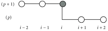
manner,𝑢(𝑝+1)_𝑖 in (23) is calculated by proceeding from the right boundary towards the left (Figure 1).

The computational molecules are depicted in Figures2 and3.

At each level of iteration, the computational molecules involve two known grid points at the new level and another three known ones at the old level. Clearly, the method is explicit.

4. Convergence Analysis of the IADEMF4

This section proves the convergence of the IADEMF4. Since

𝜆 > 1will not guarantee an accurate approximation for𝜕𝑈/𝜕𝑡

[18], the values of𝜆that are considered appropriate for the proof are0 < 𝜆 ≤ 1.

From the definitions in ((18) and (19)), the following results are obtained:

̂𝑒1= 6 (𝑐 − 1)₅ =3𝜆₂ , implying that0 < ̂𝑒1≤3₂,

̂𝑢1= 6𝑑₅ <0, 𝑙1=_{6 − ̂𝑒}6𝑏

1<0, ̂V𝑖=

6𝑒

5 > 0

for𝑖 = 1, 2, . . . , 𝑚 − 4,

̂𝑢2= 6𝑑 + 𝑙₅1̂V1 = ̂𝑢1+𝑙1₅̂V1 < ̂𝑢1, since 𝑙1̂V1< 0,

̂𝑒2= 6 (𝑐 − 1) + 𝑙₅ 1̂𝑢1 = ̂𝑒1+𝑙1₅̂𝑢1 > ̂𝑒1, since 𝑙1̂𝑢1> 0.

(25)

Simple computation shows that𝑙₁̂𝑢₁/5 < 1. Clearly,̂𝑒₂< 6.

Lemma 1. ̂𝑒𝑖in ((18)and(19)) is such that,0 < ̂𝑒𝑖 < 6, for all

𝑖 = 1, 2, 3, . . . , 𝑚 − 2.

Proof. The results in (25) show that6 > ̂𝑒₂> ̂𝑒₁> 0. Assume it is true that6 > ̂𝑒_𝑘 > ̂𝑒_𝑘−1 > 0for all𝑘 = 3, 4, 5, . . . , 𝑚 − 3. Since the assumption implies that6 > ̂𝑒_𝑘−1 > ̂𝑒_𝑘−2> 0, then

̂

𝑚_𝑘−1= 6𝑎/(6 − ̂𝑒_𝑘−1) > ̂𝑚_𝑘−2= 6𝑎/(6 − ̂𝑒_𝑘−2) > 0. Therefore,

̂

𝑚_𝑘−1̂V𝑘−1> ̂𝑚𝑘−2̂V𝑘−2.

It has also been shown that̂𝑢₂< ̂𝑢₁< 0. Assume it is true

that̂𝑢_𝑗< ̂𝑢_𝑗−1< 0 for all𝑗 = 3, 4, . . . , 𝑚 − 4. The assumption

implies that̂𝑢_𝑗−1< ̂𝑢_𝑗−2< 0. Thus,𝑚̂_𝑗−1̂𝑢_𝑗−1< ̂𝑚_𝑗−2̂𝑢_𝑗−2< 0

̂𝑢𝑗+1=

6𝑑 + 𝑙_𝑗̂V_𝑗

5 = ̂𝑢1+

𝑙_𝑗̂V_𝑗

5 = ̂𝑢1+

(6𝑏 + ̂𝑚𝑗−1̂𝑢𝑗−1) ̂V𝑗

5 (6 − ̂𝑒_𝑗)

< ̂𝑢₁+(6𝑏 + ̂𝑚𝑗−2̂𝑢𝑗−2) ̂V𝑗−1

5 (6 − ̂𝑒_𝑗−1)

= ̂𝑢₁+𝑙𝑗−1̂V𝑗−1

5 = ̂𝑢𝑗< 0.

(26)

Since it is true that, for𝑗 + 1, ̂𝑢_𝑗+1 < ̂𝑢_𝑗 < 0, then, by induction, the assumption̂𝑢_𝑗 < ̂𝑢_𝑗−1 < 0is true for all𝑗. An

0

u(p+1/2)_i

u(p+1)_i

i− 1 i i + 1 m + 1

Figure 1: The two-stage IADEMF4 algorithm. The directions of the sweeps at the(𝑝 + 1/2)and(𝑝 + 1)iteration levels.

i− 1 i

i − 2 i + 1 i + 2

(p + 1/2)

(p)

Figure 2: Computational molecule of the IADEMF4 at the(𝑝+1/2) iteration level.

i− 1 i

i − 2 i + 1 i + 2

(p + 1/2) (p + 1)

Figure 3: Computational molecule of the IADEMF4 at the(𝑝 + 1) iteration level.

equivalent to the preceding statement would bê𝑢_𝑘< ̂𝑢_𝑘−1< 0 for all𝑘 = 3, 4, 5, . . . , 𝑚 − 3. It follows that

𝑙_𝑘̂𝑢𝑘= (6𝑏 + ̂𝑚_{6 − ̂𝑒}𝑘−1̂𝑢𝑘−1) ̂𝑢𝑘

𝑘

> (6𝑏 + ̂𝑚𝑘−2̂𝑢𝑘−2) ̂𝑢𝑘−1

6 − ̂𝑒_𝑘−1 = 𝑙𝑘−1̂𝑢𝑘−1,

̂𝑒𝑘+1= 6 (𝑐 − 1) + 𝑙𝑘̂𝑢₅𝑘+ ̂𝑚𝑘−1̂V𝑘−1 = ̂𝑒1+𝑙𝑘̂𝑢𝑘+ ̂𝑚₅𝑘−1̂V𝑘−1

> ̂𝑒₁+𝑙𝑘−1̂𝑢𝑘−1+ ̂𝑚𝑘−2̂V𝑘−2

5 = ̂𝑒𝑘> 0.

(27)

Since it is true that, for𝑘+1,̂𝑒_𝑘+1> ̂𝑒_𝑘> 0, then, by induction,

̂𝑒𝑘> ̂𝑒𝑘−1> 0is also true for all𝑘.

Suppose there is a𝑘such that̂𝑒_𝑘> 6. Then,

̂𝑒𝑘+1= ̂𝑒1+𝑙𝑘̂𝑢𝑘+ ̂𝑚₅𝑘−1̂V𝑘−1

= ̂𝑒₁+ 6𝑏 + ̂𝑢𝑘

5 (6 − ̂𝑒_𝑘)+

̂

𝑚_𝑘−1

5 (

̂𝑢_𝑘−1̂𝑢_𝑘

6 − ̂𝑒𝑘 + ̂V𝑘−1) < ̂𝑒1.

(28)

This is a contradiction sincê𝑒_𝑘+1 > ̂𝑒₁. This verifies that6 >

̂𝑒𝑘 > ̂𝑒𝑘−1> 0,𝑘 = 3, 4, 5, . . . , 𝑚 − 3. Let𝑖 = 2, 3, 4, . . . , 𝑚 − 2,

and then6 > ̂𝑒_𝑖 > ̂𝑒_𝑖−1 > 0. Therefore,0 < ̂𝑒_𝑖 < 6, 𝑖 =

(6)

Lemma 2. If𝑟 > 0and𝑔 = (6 + 𝑟)/6, thenmax|(𝑟 − 𝑔̂𝑒_𝑖)/(𝑟 +

̂𝑒𝑖)| < 1, i= 1, 2, 3, . . . , 𝑚 − 2.

Proof. Let max|(𝑟 − 𝑔̂𝑒_𝑖)/(𝑟 + ̂𝑒_𝑖)| = |(𝑟 − 𝑔̂𝑒_𝑗)/(𝑟 + ̂𝑒_𝑗)|for some𝑗.

Assume|(𝑟 − 𝑔̂𝑒_𝑗)/(𝑟 + ̂𝑒_𝑗)| ≥ 1. Since𝑟 > 0and̂𝑒_𝑗 > 0,

then𝑟 + ̂𝑒_𝑗 > 0.

If(𝑟 − 𝑔̂𝑒_𝑗)/(𝑟 + ̂𝑒_𝑗) ≥ 1, then−((6 + 𝑟)/6)̂𝑒_𝑗 ≥ ̂𝑒_𝑗, which

implies that𝑟 ≤ −12. This contradicts the fact that𝑟 > 0.

If(𝑟 − 𝑔̂𝑒_𝑗)/(𝑟 + ̂𝑒_𝑗) ≤ −1, then2𝑟 − ((6 + 𝑟)/6)̂𝑒_𝑗 ≤ −̂𝑒_𝑗,

Proposition 3. ‖(𝑟𝐼 − 𝑔𝐺₁)(𝑟𝐼 + 𝐺₁)−1‖₂< 1.

Proof. Let𝐹 = (𝑟𝐼 − 𝑔𝐺₁)(𝑟𝐼 + 𝐺₁)−1; that is,

𝐹 = [ [ [ [ [ [ [ [ [ [ [

𝑟 − 𝑔 𝑑

d 𝑟 − 𝑔_𝑑 𝑂

d d d

..

. ... d d

⋅ ⋅ ⋅ ⋅ ⋅ ⋅ ⋅ ⋅ ⋅ ⋅ ⋅ ⋅ 𝑟 − 𝑔

𝑑 ] ] ] ] ] ] ] ] ] ] ]

. (29)

𝐹is a lower triangular matrix, with all the diagonal entries (whence the eigenvalues of𝐹) equal to(𝑟 − 𝑔)/𝑑, where𝑑 =

𝑟 + 1. Denote all the eigenvalues of𝐹by𝜆_𝐹. If𝜌[𝐹]is defined

as the spectral radius of𝐹, then

𝜌 [𝐹] =max󵄨󵄨󵄨󵄨𝜆_𝐹󵄨󵄨󵄨󵄨 = 󵄨󵄨󵄨󵄨𝜆_𝐹󵄨󵄨󵄨󵄨 =󵄨󵄨󵄨󵄨_󵄨󵄨󵄨𝑟 − 𝑔

𝑟 + 1󵄨󵄨󵄨󵄨󵄨󵄨󵄨 ≤ ‖𝐹‖2. (30)

But, by definition of 2-norm,

‖𝐹‖2=_‖max_x_‖2 _{̸= 0}‖𝐹_‖_xx_‖‖2

2 =‖maxy‖2=1

󵄩󵄩󵄩󵄩𝐹y󵄩󵄩󵄩󵄩2

󵄩󵄩󵄩󵄩y󵄩󵄩󵄩󵄩₂ =_‖maxy‖2=1󵄩󵄩󵄩󵄩𝐹y󵄩󵄩󵄩󵄩2

≤ max

‖w‖2=1‖𝐹w‖2=‖maxw‖2=1󵄩󵄩󵄩󵄩𝜆𝐹w󵄩󵄩󵄩󵄩2.

(31)

Since all the eigenvalues of𝐹are equal, then

‖𝐹‖₂_{≤ 󵄨󵄨󵄨󵄨𝜆}_𝐹󵄨󵄨󵄨󵄨max

‖w‖2=1‖w‖2= 󵄨󵄨󵄨󵄨𝜆𝐹󵄨󵄨󵄨󵄨 = 𝜌[𝐹]. (32)

Thus, from (30) and (32),‖𝐹‖₂ = |𝜆_𝐹| = |(𝑟 − 𝑔)/(𝑟 + 1)|. ByLemma 2 with𝑒_𝑗 replaced by 1, |(𝑟 − 𝑔)/(𝑟 + 1)| < 1 is obtained, leading to the result ofProposition 3, which is

‖𝐹‖₂= ‖(𝑟𝐼 − 𝑔𝐺₁)(𝑟𝐼 + 𝐺₁)−1‖₂< 1.

Proposition 4. ‖(𝑟𝐼 − 𝑔𝐺₂)(𝑟𝐼 + 𝐺₂)−1_‖

2< 1.

Proof. Let𝐾 = (𝑟𝐼 − 𝑔𝐺₂)(𝑟𝐼 + 𝐺₂)−1; that is,

𝐾 = [ [ [ [ [ [ [ [ [ [ [ [ [ [

𝑟 − 𝑔̂𝑒₁

𝑧1 d ⋅ ⋅ ⋅ ⋅ ⋅ ⋅ ⋅ ⋅ ⋅

𝑟 − 𝑔̂𝑒₂

𝑧₂ d ⋅ ⋅ ⋅ ...

d ... ...

𝑂 d d ...

𝑟 − 𝑔̂𝑒_𝑚

𝑧_𝑚

] ] ] ] ] ] ] ] ] ] ] ] ] ]

. (33)

𝐾is an upper triangular matrix, with all the diagonal entries equal to(𝑟 − 𝑔̂𝑒_𝑖)/𝑧_𝑖, 𝑖 = 1, 2, . . . , 𝑚 − 2, where𝑧_𝑖 = 𝑟 + ̂𝑒_𝑖. Since all the eigenvalues of𝐾are distinct, then𝐾is similar to a diagonal matrix𝐷.

By the Schur triangularization theorem [20], there is an orthogonal matrix 𝑂such that𝑂𝑇𝐾𝑂 = 𝐷. The diagonal entries of𝐷are the eigenvalues of𝐾

‖𝐾‖₂_{= 󵄩󵄩󵄩󵄩󵄩𝑂}𝑇_{𝐾𝑂󵄩󵄩󵄩󵄩󵄩2}= ‖𝐷‖2

= √maximum eigenvalue of𝐷𝑇𝐷

= √maximum eigenvalue of𝐷2

= √𝜌 (𝐷2_{) = √𝜌 (𝐾}2_{) = 𝜌 (𝐾) .}

(34)

ByLemma 2,

‖𝐾‖₂= 𝜌 (𝐾) =max󵄨󵄨󵄨󵄨󵄨󵄨󵄨󵄨𝑟 − 𝑔̂𝑒𝑖

𝑟 + ̂𝑒_𝑖 󵄨󵄨󵄨󵄨󵄨󵄨󵄨󵄨 =󵄨󵄨󵄨󵄨󵄨󵄨󵄨󵄨_󵄨󵄨

𝑟 − 𝑔̂𝑒_𝑗

𝑟 + ̂𝑒_𝑗 󵄨󵄨󵄨󵄨󵄨󵄨󵄨󵄨_󵄨󵄨< 1, (35)

for some𝑗. Hence, this provesProposition 4.

From (20) and (21),

u(𝑝+1)= (𝑟𝐼 + 𝐺₂)−1(𝑟𝐼 − 𝑔𝐺₁)

× [(𝑟𝐼 + 𝐺₁)−1(𝑟𝐼 − 𝑔𝐺₂)u(𝑝)_{+ (𝑟𝐼 + 𝐺}

1)−1f]

+ 𝑔 (𝑟𝐼 + 𝐺2)−1f.

(36)

Let

𝑀 (𝑟) = (𝑟𝐼 + 𝐺2)−1(𝑟𝐼 − 𝑔𝐺1) (𝑟𝐼 + 𝐺1)−1(𝑟𝐼 − 𝑔𝐺2) ,

(37)

And let

𝑞 (𝑟) = [(𝑟𝐼 + 𝐺2)−1(𝑟𝐼 − 𝑔𝐺1) (𝑟𝐼 + 𝐺1)−1

+𝑔(𝑟𝐼 + 𝐺₂)−1]f. (38)

Then,u(𝑝+1) = 𝑀(𝑟)u(𝑝)+ 𝑞(𝑟).

Theorem 5. The IADEMF4 is convergent if𝜌[𝑀(𝑟)] < 1, for

(7)

Proof. Define𝑀(𝑟) = (𝑟𝐼 + 𝐺̃ ₂)𝑀(𝑟)(𝑟𝐼 + 𝐺₂)−1; then

̃

𝑀 (𝑟) = (𝑟𝐼 − 𝑔𝐺1) (𝑟𝐼 + 𝐺1)−1(𝑟𝐼 − 𝑔𝐺2) (𝑟𝐼 + 𝐺2)−1.

(39)

Thus, by similarity,𝑀(𝑟)and𝑀(𝑟)̃ have the same set of eigen-values. Therefore,

𝜌 [𝑀 (𝑟)]

= 𝜌 [ ̃𝑀 (𝑟)] ≤󵄩󵄩󵄩󵄩_󵄩𝑀 (𝑟)̃ 󵄩󵄩󵄩󵄩_󵄩₂

= 󵄩󵄩󵄩󵄩󵄩(𝑟𝐼 − 𝑔𝐺1) (𝑟𝐼 + 𝐺1)−1(𝑟𝐼 − 𝑔𝐺2) (𝑟𝐼 + 𝐺2)−1󵄩󵄩󵄩󵄩_󵄩₂

≤ 󵄩󵄩󵄩󵄩󵄩(𝑟𝐼 − 𝑔𝐺1) (𝑟𝐼 + 𝐺1)−1󵄩󵄩󵄩󵄩_󵄩2_{󵄩(𝑟𝐼 − 𝑔𝐺}󵄩󵄩󵄩󵄩 2) (𝑟𝐼 + 𝐺2)−1󵄩󵄩󵄩󵄩_󵄩₂

< 1.

(40)

The last inequality is due to Propositions3and4. The proven Theorem 5assures the convergence of the IADEMF4.

5. The Fourth-Order Classical

Iterative Methods

The system of linear equations in (8) may also be solved by using the classical iterative methods of the fourth order. They include the JAC4, the GS4, and the SOR4 methods. These iterative methods are capable of exploiting the sparse structure of the pentadiagonal matrix.

The JAC4 algorithm can be represented by

𝑢(𝑝+1)_𝑖 = (𝑓𝑖−𝑎𝑢

(𝑝)

𝑖−2− 𝑏𝑢(𝑝)𝑖−1− 𝑑𝑢𝑖+1(𝑝)− 𝑒𝑢(𝑝)𝑖+2)

𝑐 ,

𝑖 = 2, 3, . . . , 𝑚 − 1.

(41)

The approximation of𝑢(𝑝+1)_𝑖 at the(𝑝 + 1)th iteration level is computed using the relevant values in the𝑝th iteration.

The GS4 method uses the most recent values of 𝑢(𝑝+1)_𝑖−2

and𝑢(𝑝+1)_𝑖−1 to update the approximation value of𝑢(𝑝+1)_𝑖 . The

algorithm for the GS4 is as expressed in (42)

𝑢(𝑝+1)_𝑖 =(𝑓𝑖−𝑎𝑢

(𝑝+1)

𝑖−2 − 𝑏𝑢(𝑝+1)𝑖−1 − 𝑑𝑢(𝑝)𝑖+1− 𝑒𝑢(𝑝)𝑖+2)

𝑐 ,

𝑖 = 2, 3, . . . , 𝑚 − 1.

(42)

The SOR4 iterative method accelerates the convergence rate of the GS4. If𝜔is a relaxation parameter, then for any

𝜔 ̸= 0, (42) can be rewritten as

𝑢_𝑖(𝑝+1)= (1 − 𝜔) 𝑢(𝑝)_𝑖

+𝜔 (𝑓𝑖− 𝑎𝑢

(𝑝+1)

𝑖−2 − 𝑏𝑢(𝑝+1)𝑖−1 − 𝑑𝑢(𝑝)𝑖+1− 𝑒𝑢(𝑝)𝑖+2)

𝑐 ,

𝑖 = 2, 3, . . . , 𝑚 − 1.

(43)

i− 1 i

i − 2 i + 1 i + 2

(p + 1)

(p)

Figure 4: Computational molecule of the JAC4.

i− 1 i

i − 2 i + 1 i + 2

(p + 1)

(p)

Figure 5: Computational molecule of the GS4/SOR4.

Table 1: Sequential arithmetic operations per iteration (𝑚: problem size).

Method Number of additions

Number of multiplications

Total operation count IADEMF4 10(𝑚 − 2) 13(𝑚 − 2) 23(𝑚 − 2)

IADEMF2 6𝑚 9𝑚 15𝑚

JAC4/GS4 4(𝑚 − 2) 5(𝑚 − 2) 9(𝑚 − 2)

SOR4 5(𝑚 − 2) 7(𝑚 − 2) 12(𝑚 − 2)

The SOR4 algorithm reduces to the GS4 if𝜔 = 1. Except for very special cases, it is difficult to obtain the analytic expression for𝜔. According to Young [21], the precise deter-mination of the optimal𝜔in the SOR is only known for a small class of matrices. The value of𝜔generally lies in the range of1 < 𝜔 < 2.

The computational molecules for the JAC4 and the GS4 are as illustrated in Figures4and5, respectively. The SOR4 has the same form as the GS4.

6. Computational Complexity

The cost of implementing an algorithm can be assessed by examining its computational complexity. The number of arithmetic operations such as additions (including subtrac-tions) and multiplications (including divisions) that is needed to perform by the algorithm can be straightforwardly count-ed.Table 1gives the number of sequential arithmetic opera-tions per iteration that is required to evaluate the algorithms. For the higher-order schemes, trade-off between accuracy and speed usually happens. The computational complexity has an effect on the efficiency of a particular scheme. Thus, this factor will be taken into account when discussing the results of the numerical experiments conducted in this study.

7. The Pseudocode of the IADEMF4

Sequential Algorithm

(8)

begin

determine the parameters𝑚, 𝑟, Δ𝑡, Δ𝑥, 𝜆, 𝜀, 𝑇 determine initial conditions𝑢_𝑖(𝑝)

determine exact solutions𝑈_𝑖at time level𝑇

while(time level< 𝑇)

determine boundary conditions

for𝑖 = 2to𝑖 = 𝑚 − 1

compute𝑓_𝑖(refer to (9))

end-for

set iteration = 0

while(convergence conditions are not satisfied)

for𝑖 = 2to𝑖 = 𝑚 − 1

compute𝑢(𝑝+1/2)_𝑖 (refer to (22))

end-for

for𝑖 = 2to𝑖 = 𝑚 − 1

compute𝑢(𝑝+1)_𝑖 (refer to (23))

end-for

test for convergence: compute𝑒_𝑖← 󵄨󵄨󵄨󵄨󵄨𝑢(𝑝+1)_𝑖 − 𝑢(𝑝)_𝑖 󵄨󵄨󵄨󵄨_󵄨

if(max󵄨󵄨󵄨󵄨𝑒_𝑖󵄨󵄨󵄨󵄨 < 𝜀)

then𝑢(𝑝)_𝑖 ← 𝑢(𝑝+1)_𝑖

add 1 to iteration (if necessary)

end-while end-while

for𝑖 = 2to𝑖 = 𝑚 − 1

determine average absolute error, root mean square error and maximum error

end-for end

Algorithm 1: The IADEMF4 sequential algorithm.

8. Numerical Experiments

Two experiments were conducted to test the sequential numerical performance of the proposed IADEMF4 method against those of the benchmarked classical iterative methods, namely, the JAC4, the GS4, and the SOR4. Comparison is also made with the corresponding IADE method of the second order.

Experiment 1. This problem was taken from Saulev [22]

𝜕𝑈

𝜕𝑡 =

𝜕2𝑈

𝜕𝑥2, 0 ≤ 𝑥 ≤ 1 (44)

subject to the initial condition

𝑈 (𝑥, 0) = 4𝑥 (1 − 𝑥) , 0 ≤ 𝑥 ≤ 1 (45)

and the boundary conditions

𝑈 (0, 𝑡) = 𝑈 (1, 𝑡) = 0, 𝑡 ≥ 0. (46)

The exact solution to the given problem is given by

𝑈 (𝑥, 𝑡) = 32_𝜋₃ ∑∞

𝑘=1,(2) 1

𝑘3 𝑒−𝜋

2_𝑘2_𝑡

sin(𝑘𝜋𝑥) . (47)

Experiment 2. This problem was taken from Johnson and Reiss [23],

𝜕𝑈

𝜕𝑡 =

𝜕2_𝑈

𝜕𝑥2, 0 ≤ 𝑥 ≤ 1 (48)

subject to the initial condition

𝑈 (𝑥, 0) =sin(𝜋𝑥) (1 + 6cos(𝜋𝑥)) , 0 ≤ 𝑥 ≤ 1 (49)

and the boundary conditions

𝑈 (0, 𝑡) = 𝑈 (1, 𝑡) = 0, 𝑡 ≥ 0. (50)

The exact solution to the given problem is given by

(9)

9. Results and Discussion

In each experiment, the exact solutions at𝑖 = 1and𝑖 = 𝑚 were taken as boundary values for the IADEMF4 and the other fourth-order classical iterative methods. The conver-gence criterion used in the testing of each method was taken

as‖𝑢(𝑝+1)− 𝑢(𝑝)‖_∞≤ 𝜀, where 𝜀is the convergence tolerance.

The selections of the optimum𝑟 or𝜔were determined by experiments. As for the IADEMF2, the CN scheme with𝜃 =

1/2was employed.

Figures6, 7, 8, and9visualize the behavior of the one-dimensional parabolic heat solutions for both experiments. By using𝑚 = 10and a tolerance requirement of𝜀 = 10−4, two different mesh sizes,𝜆 = 0.5and 𝜆 = 1.0, were considered in each experiment. The exact solutions are compared with the IADEMF4 and the IADEMF2 numerical solutions. The optimum value of𝑟chosen for each method, as well as their corresponding outcome of the number of iterations, 𝑛, is stated in the legend of each figure. Every figure reveals that the IADEMF4 is more accurate than the IADEMF2 and the former converges with fewer numbers of iterations in comparison to the latter. The numerical solutions of the IADEMF4 seem to be in very good agreement with the exact solutions. For example, in Figure 7, at𝑥 = 0.5, the difference between the exact solution and the numerical solution using the IADEMF2 and using the IADEMF4 is about 3.6% and 0%, respectively. These results imply that the accuracy and convergence rate of the second-order IADE method are enhanced by the implementation of the fourth-order CN approximation that leads to the formation of the corresponding fourth-order IADE scheme.

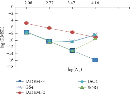
Figure 10displays the graph of log (RMSE) versus log(Δ𝑥) for decreasing values ofΔ𝑥implemented on Experiment 2. By considering𝜀 = 10−4and fixingΔ𝑡 = 0.0001, the value of

Δ𝑥was initially taken asΔ𝑥 = 0.125. It was then successively halved intoΔ𝑥/2,Δ𝑥/4, andΔ𝑥/8.

The figure shows that amongst the tested methods, the root mean square error (RMSE) of the IADEMF4 and the IADEMF2 decreases linearly as the values ofΔ𝑥decreases. The slope of the IADEMF4 is approximately equal to 4, which corresponds to its fourth-order spatial accuracy. The IADEMF2 with a second-order spatial accuracy has a slope that is approximately equal to 2. It is clear that the IADEMF4 is always more accurate than the IADEMF2, for the different considered mesh sizes. The graphs of the SOR4(𝜔 = 1.05), the GS4, and the JAC4 show that their accuracies of fourth order tend to lack asΔ𝑥decreases, largely due to the effect of increasing round-off errors as the value of𝑚increases.

Tables2,3,4,5,6,7,8, and9provide numerical results in terms of the average absolute error (AAE), root mean square error (RMSE), maximum error (ME), number of iterations

(𝑛), and execution time (ET) measured in seconds (s). The results are obtained from both experiments for two different values of𝑚and mesh size, 𝜆. It is generally observed that

when𝑚 = 700, 𝜆 = 0.5, and 𝜀 = 10−6, the IADEMF4

has the least average absolute error, root mean square error, and maximum error in comparison with the other methods under consideration (Tables2–5). When the size of𝑚was

0 0.1 0.2 0.3 0.4 0.5 0.6 0.7 0.8 0.9 1

x

Exact solution

IADEMF4(r = 0.8, n = 172)

IADEMF2(r = 0.3, n = 185)

0.0E + 00 1.0E − 02 2.0E − 02 3.0E − 02 4.0E − 02 5.0E − 02 6.0E − 02 7.0E − 02 8.0E − 02 9.0E − 02 1.0E − 01

U(

x,

t)

Figure 6: Numerical and exact solutions forExperiment 1.𝜆 = 0.5,

Δ𝑥 = 0.1,Δ𝑡 = 0.005,𝑡 = 0.25, and𝜀 = 10−4.

0 0.1 0.2 0.3 0.4 0.5 0.6 0.7 0.8 0.9 1

x

Exact solution

IADEMF4(r = 1.4, n = 159)

IADEMF2(r = 0.5, n = 162)

0.0E + 00 1.0E − 03 2.0E − 03 3.0E − 03 4.0E − 03 5.0E − 03 6.0E − 03 7.0E − 03 8.0E − 03 9.0E − 03

U(

x,

t)

Δ𝑥 = 0.1,Δ𝑡 = 0.01,𝑡 = 0.5, and𝜀 = 10−4.

ten times bigger(𝑚 = 7000)and a more stringent tolerance criterion was set(𝜀 = 10−10), the accuracy of the IADEMF4 clearly outperforms the other methods for a mesh size of

𝜆 = 0.5(Tables6and8). However, the difference in the errors

amongst the tested methods is not so obvious for the case of

𝜆 = 1.0(Tables7and9). The achievement of the fourth-order

IADE method in Experiments1and2can be clearly seen from the results in Tables2and8, respectively, where it has caused a huge 94% reduction of RMSE from its corresponding second-order IADE method.

(10)

0 0.1 0.2 0.3 0.4 0.5 0.6 0.7 0.8 0.9 1

x

Exact solution

IADEMF4(r = 1.0, n = 169)

IADEMF2(r = 0.3, n = 213)

0.0E + 00 1.0E − 02 2.0E − 02 3.0E − 02 4.0E − 02 5.0E − 02 6.0E − 02 7.0E − 02 8.0E − 02 9.0E − 02 1.0E − 01

U(

x,

t)

Δ𝑥 = 0.1,Δ𝑡 = 0.005,𝑡 = 0.25, and𝜀 = 10−4.

0 0.1 0.2 0.3 0.4 0.5 0.6 0.7 0.8 0.9 1

x

Exact solution

IADEMF4(r = 1.0, n = 175)

IADEMF2(r = 0.5, n = 182)

0.0E + 00 1.0E − 03 2.0E − 03 3.0E − 03 4.0E − 03 5.0E − 03 6.0E − 03 7.0E − 03 8.0E − 03

U(

x,

t)

Δ𝑥 = 0.1,Δ𝑡 = 0.01,𝑡 = 0.5, and𝜀 = 10−4.

The IADEMF2 is only derived from the second-order CN approximation, but its combination with its corresponding fourth-order MF variant managed to produce errors which are better than the GS4, JAC4, and the SOR4. Even though the classical iterative methods are also derived from the fourth-order accurate CN type approximation, they are lacking in accuracy due to the round-off errors that have been accumulated from the time the execution starts till it ends.

With regards to the rate of convergence, the results from each table demonstrate that the number of iterations produced by the IADEMF2 and the fourth-order classical iterative methods is greater than or at least equal to that of

0 −2

−2.08 −2.77 −3.47 −4.16

−4

−8 −6

−10 −12 −14 −16 −18

GS4

JAC4

SOR4

log (RMS

E)

log(Δx)

IADEMF4

IADEMF2

Figure 10: Log(RMSE) versus Log(Δ𝑥)Experiment 2.Δ𝑡 = 0.0001,

𝑡 = 0.002, and𝜀 = 10−4.

Table 2:Experiment 1.𝑚 = 700,𝜆 = 0.5,Δ𝑥 = 1.43 × 10−3,Δ𝑡 =

1.02 × 10−6_,_{𝑡 = 5.09 × 10}−5_{, and}_{𝜀 = 10}−6_.

Method AAE RMSE ME 𝑛 ET (s)

IADEMF4

(𝑟 = 0.7) 2.67𝑒 − 9 3.30𝑒 − 9 2.12𝑒 − 8 100 4.40𝑒 − 2

IADEMF2

(𝑟 = 0.8) 1.88𝑒 − 8 4.95𝑒 − 8 3.23𝑒 − 7 100 6.35𝑒 − 3

SOR4

(𝜔 = 1.2) 5.40𝑒 − 7 5.44𝑒 − 7 5.52𝑒 − 7 108 4.60𝑒 − 2

GS4 5.40𝑒 − 6 5.43𝑒 − 6 3.32𝑒 − 6 150 4.72𝑒 − 2

JAC4 2.28𝑒 − 5 2.29𝑒 − 5 2.32𝑒 − 5 150 4.73𝑒 − 2

2.04 × 10−6_,_{𝑡 = 5.09 × 10}−5_{, and}_{𝜀 = 10}−6_.

IADEMF4

(𝑟 = 1.0) 2.97𝑒 − 7 3.01𝑒 − 7 3.01𝑒 − 7 50 2.01𝑒 − 2

IADEMF2

(𝑟 = 0.9) 5.57𝑒 − 7 5.59𝑒 − 7 8.48𝑒 − 7 50 3.17𝑒 − 3

SOR4

(𝜔 = 1.2) 3.29𝑒 − 6 3.31𝑒 − 6 3.35𝑒 − 6 76 2.25𝑒 − 2

GS4 8.95𝑒 − 6 9.00𝑒 − 6 9.00𝑒 − 6 100 2.38𝑒 − 2

JAC4 2.14𝑒 − 5 2.15𝑒 − 5 2.17𝑒 − 5 125 2.50𝑒 − 2

(11)

1.02 × 10−6_,_{𝑡 = 5.09 × 10}−5_{, and}_{𝜀 = 10}−6_.

Method AAE RMSE ME n ET (s)

IADEMF4

(𝑟 = 0.7) 2.07𝑒 − 8 2.31𝑒 − 8 3.45𝑒 − 8 100 9.03𝑒 − 3

IADEMF2

(𝑟 = 0.8) 1.06𝑒 − 7 1.75𝑒 − 7 1.75𝑒 − 7 100 6.47𝑒 − 3

SOR4

(𝜔 = 1.1) 1.54𝑒 − 6 1.71𝑒 − 6 2.55𝑒 − 6 200 1.10𝑒 − 2

GS4 2.94𝑒 − 6 3.27𝑒 − 6 4.87𝑒 − 6 250 1.18𝑒 − 2

JAC4 1.24𝑒 − 5 1.38𝑒 − 5 2.06𝑒 − 5 300 1.27𝑒 − 2

2.04 × 10−6_,_{𝑡 = 5.09 × 10}−5_{, and}_{𝜀 = 10}−6_.

IADEMF4

(𝑟 = 0.9) 1.38𝑒 − 6 1.54𝑒 − 6 2.29𝑒 − 6 75 6.50𝑒 − 3

IADEMF2

(𝑟 = 0.5) 1.87𝑒 − 6 2.07𝑒 − 6 3.09𝑒 − 6 75 4.72𝑒 − 3

SOR4

(𝜔 = 1.2) 3.12𝑒 − 6 3.47𝑒 − 6 5.17𝑒 − 6 125 9.06𝑒 − 3

GS4 6.67𝑒 − 6 7.42𝑒 − 6 1.11𝑒 − 5 175 9.32𝑒 − 3

JAC4 1.26𝑒 − 5 1.41𝑒 − 5 2.10𝑒 − 5 250 1.05𝑒 − 2

1.02 × 10−8_,_{𝑡 = 5.10 × 10}−7_{, and}_{𝜀 = 10}−10_.

Method AAE RMSE ME n ET (s)

IADEMF4

(𝑟 = 0.8) 3.67𝑒 − 10 4.33𝑒 − 10 3.66𝑒 − 9 173 1.46𝑒 − 1

IADEMF2

(𝑟 = 0.5) 3.75𝑒 − 10 4.35𝑒 − 10 3.76𝑒 − 9 200 1.24𝑒 − 1

SOR4

(𝜔 = 1.12) 4.55𝑒 − 10 5.07𝑒 − 10 3.67𝑒 − 9 257 1.47𝑒 − 1

GS4 1.10𝑒 − 9 1.11𝑒 − 9 3.76𝑒 − 9 300 1.60𝑒 − 1

JAC4 2.30𝑒 − 9 2.31𝑒 − 9 3.78𝑒 − 9 400 1.63𝑒 − 1

2.04 × 10−8_,_{𝑡 = 5.1 × 10}−7_{, and}_{𝜀 = 10}−10_.

IADEMF4

(𝑟 = 1.0) 1.63𝑒 − 7 1.63𝑒 − 7 1.63𝑒 − 7 112 9.60𝑒 − 2

IADEMF2

(𝑟 = 1.2) 1.63𝑒 − 7 1.63𝑒 − 7 1.63𝑒 − 7 120 7.36𝑒 − 2

SOR4

(𝜔 = 1.15) 1.63𝑒 − 7 1.63𝑒 − 7 1.64𝑒 − 7 171 9.99𝑒 − 2

GS4 1.64𝑒 − 7 1.64𝑒 − 7 1.64𝑒 − 7 216 1.07𝑒 − 1

JAC4 1.65𝑒 − 7 1.65𝑒 − 7 1.65𝑒 − 7 312 1.11𝑒 − 1

It is found that the convergence rate of the fourth-order and second-order methods improves with the application of larger mesh size, that is, from 𝜆 = 0.5 to 𝜆 = 1.0. The coarser meshes cause a reduction in the computational oper-ations, thus giving better rate of convergence. However, a

1.02 × 10−8_,_{𝑡 = 5.10 × 10}−7_{, and}_{𝜀 = 10}−10_.

IADEMF4

(𝑟 = 0.7) 5.67𝑒 − 13 3.21𝑒 − 12 1.30𝑒 − 10 150 1.31𝑒 − 1

IADEMF2

(𝑟 = 0.7) 1.99𝑒 − 11 4.60𝑒 − 11 1.82𝑒 − 9 200 1.27𝑒 − 1

SOR4

(𝜔 = 1.15) 2.45𝑒 − 10 2.73𝑒 − 10 3.99𝑒 − 10 260 1.51𝑒 − 1

GS4 3.98𝑒 − 10 4.43𝑒 − 10 6.61𝑒 − 10 400 1.71𝑒 − 1

JAC4 1.05𝑒 − 9 1.17𝑒 − 9 1.74𝑒 − 9 550 1.76𝑒 − 1

2.04 × 10−8_,_{𝑡 = 5.1 × 10}−7_{, and}_{𝜀 = 10}−10_.

IADEMF4

(𝑟 = 1.0) 1.54𝑒 − 6 1.71𝑒 − 6 2.55𝑒 − 6 96 9.12𝑒 − 2

IADEMF2

(𝑟 = 1.0) 1.54𝑒 − 6 1.71𝑒 − 6 2.55𝑒 − 6 96 6.07𝑒 − 2

SOR4

(𝜔 = 1.2) 1.54𝑒 − 6 1.71𝑒 − 6 2.55𝑒 − 6 192 9.97𝑒 − 2

GS4 1.54𝑒 − 6 1.71𝑒 − 6 2.55𝑒 − 6 288 1.28𝑒 − 1

JAC4 1.54𝑒 − 6 1.72𝑒 − 6 2.56𝑒 − 6 408 1.46𝑒 − 1

more accurate solution is obtained by using finer mesh. For example,Table 6shows that, for𝜆 = 0.5, the IADEMF4 has

RMSE= 4.33𝑒 − 10and𝑛 = 173, whereasTable 7shows that,

for𝜆 = 1.0, its RMSE = 1.63𝑒 − 7and𝑛 = 112. In general,

amongst all the tested methods, the IADEMF4 still maintains its greater accuracy characteristic, even with coarser meshes. In terms of execution time, the results from every table display shorter execution time for the IADEMF2 in compari-son to the IADEMF4. This is expected, since the IADEMF2 has lower computational complexity (Table 1). Despite the achievement in accuracy, the IADEMF4 has to perform more computational work than the IADEMF2 since the former has to utilize values of𝑢at two grid points on either side of the point(𝑖Δ𝑥, 𝑘Δ𝑡)along the𝑘th time level. Thus, if accuracy is desired, then the preferred sequential numerical algorithm would be the IADEMF4. On the other hand, if execution time matters, then the choice would be the IADEMF2.

Amongst the fourth-order methods, the IADEMF4 exe-cutes in the least amount of time. Even though its computa-tional complexity is relatively large, it operates with the least number of iterations, thus enabling it to be the most efficient.

10. Conclusion

(12)

the fourth-order IADE scheme’s higher computational com-plexity, this technique is proved to be valuable because it enhances the accuracy of its second-order counterpart, namely, the IADEMF2. In addition, the higher accuracy of IADEMF4 is verified as a convergent and unconditionally stable scheme and is superior in terms of rate of convergence. It has also been proven to execute more efficiently in compar-ison to the other benchmarked fourth-order classical iterative methods, such as the GS4, the SOR4, and the JAC4. The in-creasing number of correct digits at each iteration serves as an advantage for the IADEMF4, thus yielding faster rate of con-vergence with higher level of accuracy.

In conclusion, the proposed IADEMF4 scheme affords users many advantages with respect to higher accuracy, sta-bility, and rate of convergence, and it serves as an alternative, efficient technique for the solution of a one-dimensional heat equation with Dirichlet boundary conditions.

The proposed fourth-order scheme can be modified and adapted to more general multidimensional linear and non-linear parabolic, elliptic, and hyperbolic partial differential equations, using different types of boundary conditions. Besides, it can also be considered for applications in problems that require higher-order accuracy with high resolution, such as problems in nanocomputing that require the solution of very large sparse systems of equation.

The explicit and high accuracy feature of the IADEMF4 can be exploited in two- and three-dimensional heat prob-lems, by applying the scheme as pentadiagonal solvers for the system of linear equations arising in the sweeps of a higher-order alternating direction implicit (ADI) scheme. The lower-order ADI scheme was initially proposed by Peaceman and Rachford [24]. The higher space dimensions are expected not to cause unsatisfactory performance for the ADI-IADEMF4, as long as the proposed scheme is stable, convergent, and efficient as the process of its implementa-tion continues to advance from one-time step to another. Pathirana et al. [25] implemented the ADI in developing a two-dimensional model for incorporating flood damage in urban drainage planning. The proposed model is found to be stable, numerically accurate, and computationally efficient. Mirzavand et al. [26] proposed the ADI-FDTD method for the physical modeling of high-frequency semiconductor devices. The approach is able to reduce significantly the full-wave simulation time.

It is possible to parallelize the IADEMF4 algorithm since the calculation of the new iteration only depends on the known values from the last iteration (Figures2and3). Future work is to exploit the explicit computational properties and efficiency of the IADEMF4 for parallelization and execution on distributed parallel computing systems. The idea is to speed up the execution time without compromising its accu-racy, especially on problems involving very large linear sys-tems of equations.

References

[1] J. Noye,Computational Techniques for Differential Equations, vol. 83, Elsevier Science, North-Holland Publishing, Amster-dam, The Netherlands, 1984.

[2] G. W. Recktenwald, “Finite difference approximations to the heat equation,”Mechanical Engineering, vol. 10, pp. 1–27, 2004. [3] P. Lax and B. Wendroff, “Systems of conservation laws,”

Com-munications on Pure and Applied Mathematics, vol. 13, pp. 217– 237, 1960.

[4] R. J. MacKinnon and G. F. Carey, “Analysis of material interface discontinuities and superconvergent fluxes in finite difference theory,”Journal of Computational Physics, vol. 75, no. 1, pp. 151– 167, 1988.

[5] R. Hixon and E. Turkel,High Accuracy Compact MacCormack-Type Schemes For Computational Aerocoustics, NASA Centre for Aerospace Information, Lewis Research Centre, 1998. [6] Y. Lin,Higher-order finite difference methods for solving heat

equations [Ph.D. thesis], Southern Illinois University, 2008. [7] J. Sulaiman, M. K. Hasan, M. Othman M, and S. A. Abdul

Karim, “Fourth-order QSMOR iterative method for the solu-tion of one-dimensional parabolic PDE’s,” inProceedings of the International Conference on Industrial and Applied Mathematics (CIAM ’10), pp. 34–39, ITB, Bandung, Indonesia, 2010. [8] N. Jha, “The application of sixth order accurate parallel

quar-ter sweep alquar-ternating group explicit algorithm for nonlinear boundary value problems with singularity,” inProceedings of the 2nd International Conference on Methods and Models in Computer Science (ICM2CS ’10), pp. 76–80, December 2010. [9] Y. Jin, G. Jin, and J. Li, “A class of high-precision finite difference

parallel algorithms for convection equations,”Journal of Conver-gence Information Technology, vol. 6, no. 1, pp. 79–82, 2011. [10] W. Fu and E. L. Tan, “Development of split-step FDTD method

with higher-order spatial accuracy,”Electronics Letters, vol. 40, no. 20, pp. 1252–1253, 2004.

[11] A. Mohebbi and M. Dehghan, “High-order compact solution of the one-dimensional heat and advection-diffusion equations,”

Applied Mathematical Modelling, vol. 34, no. 10, pp. 3071–3084, 2010.

[12] W. Liao, “An implicit fourth-order compact finite difference scheme for one-dimensional Burgers’ equation,”Applied Math-ematics and Computation, vol. 206, no. 2, pp. 755–764, 2008. [13] Z. F. Tian and Y. B. Ge, “A fourth-order compact ADI method

for solving two-dimensional unsteady convection-diffusion problems,”Journal of Computational and Applied Mathematics, vol. 198, no. 1, pp. 268–286, 2007.

[14] C. Chun, “Some fourth-order iterative methods for solving non-linear equations,”Applied Mathematics and Computation, vol. 195, no. 2, pp. 454–459, 2008.

[15] S. Zhu, Z. Yu, and J. Zhao, “A high-order parallel finite difference algorithm,”Applied Mathematics and Computation, vol. 183, no. 1, pp. 365–372, 2006.

[16] Z. Gao and S. Xie, “Fourth-order alternating direction implicit compact finite difference schemes for two-dimensional Schr¨odinger equations,”Applied Numerical Mathematics, vol. 61, no. 4, pp. 593–614, 2011.

[17] M. S. Sahimi, A. Ahmad, and A. A. Bakar, “The Iterative Alter-nating Decomposition Explicit (IADE) method to solve the heat conduction equation,”International Journal of Computer Mathematics, vol. 47, pp. 219–229, 1993.

[18] G. D. Smith,Numerical Solution of Partial Differential Equa-tions: Finite Difference Methods, Oxford University Press, 2nd edition, 1978.

(13)

[20] B. N. Datta,Numerical Linear Algebra and Applications, Brooks/ Cole Publishing, Pacific Grove, Calif, USA, 1995.

[21] D. M. Young,Iterative Solution of Large Linear Systems, Aca-demic Press, New York, NY, USA, 1971.

[22] V. K. Saulev,Integration of Equations of Parabolic Type by the Method of Nets, Pergamon Press, Oxford, UK, 1964.

[23] L. W. Johnson and R. D. Riess,Numerical Analysis, Addison-Wesley, Reading, Mass, USA, 2nd edition, 1982.

[24] D. W. Peaceman and H. H. Rachford, Jr., “The numerical solu-tion of parabolic and elliptic differential equasolu-tions,”Journal of the Society for Industrial and Applied Mathematics, vol. 3, pp. 28–41, 1955.

[25] A. Pathirana, S. Tsegaye, B. Gersonius, and K. Vairavamoorthy, “A simple 2-D inundation model for incorporating flood dam-age in urban draindam-age planning,”Hydrology and Earth System Sciences, vol. 15, no. 8, pp. 2747–2761, 2011.

(14)

Submit your manuscripts at

http://www.hindawi.com

Operations

Research

Advances in

Hindawi Publishing Corporation

http://www.hindawi.com Volume 2013

http://www.hindawi.com Volume 2013 Mathematical Problems in Engineering

Abstract and

Applied Analysis

ISRN

Applied Mathematics

International Journal of

Combinatorics

http://www.hindawi.com Volume 2013 Journal of Function Spaces and Applications

International Journal of Mathematics and Mathematical Sciences

Hindawi Publishing Corporation http://www.hindawi.com Volume 2013

ISRN

Geometry

Discrete Dynamics in Nature and Society Hindawi Publishing Corporation

Advances in

Mathematical Physics

ISRN

Algebra

Probability

and

Statistics

Journal of

ISRN

Mathematical Analysis Hindawi Publishing Corporation

Journal of

Applied Mathematics

Sciences

Stochastic Analysis

http://www.hindawi.com Volume 2013 Hindawi Publishing Corporation

The Scientific

World Journal

http://www.hindawi.com Volume 2013 ISRN

Discrete Mathematics

Hindawi Publishing Corporation http://www.hindawi.com