Capturing Truthiness:
Mining Truth Tables in Binary Datasets
Clifford Conley Owens, T. M. Murali, and Naren Ramakrishnan
Department of Computer Science, Virginia Tech, VA 24061, USA
Email:
{ibcliffo,murali,naren
}@cs.vt.edu
ABSTRACT
We introduce a new data mining problem: mining truth ta-bles in binary datasets. Given a matrix of objects and the properties they satisfy, a truth table identifies a subset of properties that exhibit maximal variability (and hence, com-plete independence) in occurrence patterns over the underly-ing objects. This problem is relevant in many domains, e.g., bioinformatics where we seek to identify and model inde-pendent components of combinatorial regulatory pathways, and in social/economic demographics where we desire to de-termine independent behavioral attributes of populations. Besides intrinsic interest in such patterns, we show how the problem of mining truth tables is dual to the problem of mining redescriptions, in that a set of properties involved in a truth table cannot participate in any possible redescrip-tion. This allows us to adapt our algorithm to the problem of mining redescriptions as well, by first identifying regions where redescriptions cannot happen, and then pursuing a divide and conquer strategy around these regions. Further-more, our work suggests dual mining strategies where both classes of algorithms can be brought to bear upon either data mining task. We outline a family of levelwise approaches adapted to mining truth tables, algorithmic optimizations, and applications to bioinformatics and political datasets.
Categories and Subject Descriptors: H.2.8 [Database Management]: Database Applications - Data Mining; I.2.6 [Artificial Intelligence]: Learning
General Terms:Algorithms.
Keywords: truth tables, levelwise algorithms, indepen-dence models.
1.
INTRODUCTION
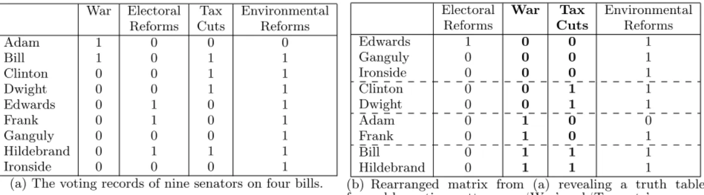
Consider the dataset shown in Fig. 1(a), which outlines nine hypothetical senators and their votes (1 for yes, 0 for no) on four bills. Given binary matrices such as these, our goal in this paper is to identify a truth table embedded inside them. Our first observation is that, given nine rows, we can
Permission to make digital or hard copies of all or part of this work for personal or classroom use is granted without fee provided that copies are not made or distributed for profit or commercial advantage and that copies bear this notice and the full citation on the first page. To copy otherwise, to republish, to post on servers or to redistribute to lists, requires prior specific permission and/or a fee.
KDD’07,August 12–15, 2007, San Jose, CA, USA. Copyright 2007 ACM X-XXXXX-XX-X/XX/XX ...$5.00.
find truth tables having at most blog2(9)c = 3 bills.
How-ever, the reader can verify that no such truth table exists. In fact, the only two truth table present is a two-column one, spanning the bills ‘War’ and ‘Tax Cuts,’ as shown in Figure 1(b). This truth table suggests that these two bills constitute independent dimensions along which politicians distinguish themselves. Observe that the senators partition into four (22) disjoint subsets with each subset having at least two senators. We separate these subsets using dashed lines in Figure 1(b).
This problem of finding truth tables can be considered or-thogonal to mining association rules [1], correlations [21], or redescriptions [13] which capture various forms of attribute dependencies and overlaps. From the perspective of these works, truth tables constitute an ‘anti-pattern,’ i.e., the vari-ables participating in it defy similarity judgements, and are hence interesting. (Later we show how truth tables can be harnessed to find patterns of similarity as well).
Several application domains possess characteristics that are amenable to truth table mining. In bioinformatics, we are given a matrix of genes (rows) versus transcription fac-tors (columns), where a 1 indicates that the transcription factor binds upstream of the given gene, and regulates it (0 otherwise). A truth table in such a matrix indicates a set of transcription factors that can be recruited in arbi-trary combinations to regulate genes. This further suggests that they are likely to form independent components of reg-ulatory pathways. Similar relationships underlie signaling pathway analysis [10] and exploration of therapies for drug discovery [3].
As a second example, consider the domain of recommender systems where the rows denote people, the columns denote movies, and a 1/0 indicates approval/disliking (assume for now that everybody has seen and rated every movie). When a new person joins the system, a typical problem faced in recommenders is to identify a (small) set of movies that this new person should be requested to rate, in order to be connected to the underlying social network of users. By identifying a truth table in the original matrix, we can learn a set of movies that serve to maximally distinguish a user from others, and hence situate the user in a suitable neigh-borhood. Thus, the ratings for these movies are the most informative questions to ask a new user. This application directly maps to recommender system designs like Jester [6] which request all users to rate the same set of artifacts. Truth table mining identifies what these artifacts should be. A truth table can be viewed as a partition of rows where each block in the partition is a ‘constant-row’ bicluster [9].
War Electoral Tax Environmental
Reforms Cuts Reforms
Adam 1 0 0 0 Bill 1 0 1 1 Clinton 0 0 1 1 Dwight 0 0 1 1 Edwards 0 1 0 1 Frank 0 1 0 1 Ganguly 0 0 0 1 Hildebrand 0 1 1 1 Ironside 0 0 0 1
(a) The voting records of nine senators on four bills.
Electoral War Tax Environmental
Reforms Cuts Reforms
Edwards 1 0 0 1 Ganguly 0 0 0 1 Ironside 0 0 0 1 Clinton 0 0 1 1 Dwight 0 0 1 1 Adam 0 1 0 0 Frank 0 1 0 1 Bill 0 1 1 1 Hildebrand 0 1 1 1
(b) Rearranged matrix from (a) revealing a truth table formed by voting patterns on ‘War’ and ‘Tax cuts’.
Figure 1: Example dataset for truth table mining.
The most familiar type of constant-row patterns are those where all cells are 1, and such biclusters correspond to item-sets as studied in association mining. Hence algorithms for mining truth tables must explicitly and necessarily keep track of an exponentially greater number of occurrence pat-terns than algorithms for mining associations. At the same time, truth tables expose several structural constraints that can be harnessed to create effective algorithms. In particu-lar, although the definition of the underlying pattern is more complicated, we show how the search for truth tables can be structured levelwise, drawing upon established notions from data mining.
“Truthiness” [20] is a term coined by television comedian Stephen Colbert to describe things that a person claims to know intuitively, instinctively, or “from the gut.” The Newspeak word “bellyfeel” [19] has similar connotations. The truth tables we compute have high truthiness, which we capture using two parameters: (i) we insist that each pattern of occurrences occur in as many rows as demanded by abalancecriterion; (ii) however, we allow a small num-ber of patterns to appear in fewer rows, controlled using the
supportparameter. More information on these parameters is provided in Section 2.
Our main contributions in this paper are:
1. We formulate truth table mining as a new data min-ing task, with associated algorithms and applications. We define the notions of balance and support to char-acterize the quality of a truth table. These notions smoothly decrease with an increase in the number of properties in a truth table.
2. We give theoretical insights into the relationships be-tween truth tables and redescriptions [22] and cast these as duals of each other. This allows us to adapt insights from algorithms for mining one type of pattern toward mining the other type of pattern.
3. We present experimental results on both synthetic and real-world datasets, helping demonstrate the scalabil-ity of our implementation and also shedding domain-specific insight.
Section 2 formally defines the truth table mining problem and Section 3 outlines how our definitions of balance and support lend themselves to levelwise search algorithms. Sec-tion 4 describes the levelwise algorithm in detail, along with some associated optimizations for improving efficiency. Sec-tion 5 presents relaSec-tionships to redescripSec-tion mining and
outlines the context in which it is dual to truth table mining. Section 6 gives experimental results on both synthetic and real-world datasets. Sections 7 and 8 provide comparisons to related work and offer a discussion, respectively.
2.
PROBLEM FORMULATION
LetOdenote a set ofnobjects,P a set ofmproperties, andR⊆O×P a relation that connects objects to proper-ties they contain. We are interested in identifying complete independence in the occurrence of subsets ofP among the objects in O. Let Q ⊆ P denote a subset of properties. Given any object o ∈ O, let oQ denote the binary vector
with |Q|elements given by the values of the properties in Q ino.Since there are 2|Q| possible distinct values of this binary vector, Q partitions the objects in O into at most 2|Q|
equivalence classes. LetEQdenote this partition. Each
element ofEQis a set of objects and each object appears in
precisely one element ofEQ. Atruth tableis a pair (Q, EQ),
whereQ⊆P and|EQ|= 2|Q|.
Note that if no two properties in P are identical (i.e., both properties appear in precisely the same set of objects), a truth table (Q, EQ) is naturally closed: by definition, the
truth table includes all objects and any property inP−Q will induce a refinement of EQ if added toQ. Henceforth,
we will abuse notation and useQto refer both to a subset of properties and the induced truth table.
Truth tables have natural notions of balance and support, which we define next. Ideally, in a truth table (Q, EQ),
each subset of objects inEQwill have size at leastbn/2|Q|c.
To accommodate deviations from this ideal, we define the
balance β(Q) of (Q, EQ) to be the quantity
β(Q) = minS∈EQ|S|
n .
Thus, every element ofEQcontains at leastβ(Q)nobjects.
Values of balance range between 0 and 1/2|Q|. Given a bal-ance threshold 0 ≤b ≤1, we say that a truth table Q is
balanced ifβ(Q)≥b. As we will show in the next two sec-tions, our definition of balance is anti-monotone, a property we exploit in our truth table mining algorithms.
Observe that we could have defined balance in a way that normalised it with respect to the number of properties inQ, e.g.,β(Q) = minSn/2∈EQk |S|. In this case, althoughβ(Q) ranges
between 0 and 1, it does not exhibit anti-monotonicity. In particular, a version of Lemma 3.2 below does not hold for this definition.
We also desire to mine ‘almost truth tables,’ where most, but not all, of the presence/absence combinations of proper-ties satisfy the balance constraint. Given a balance thresh-oldb, we define thesupportσ(Q, b) of a truth table (Q, EQ)
with balance at leastbto be the fraction of possible object sets whose size is at leastbn, i.e.,
σ(Q, b) = |{S∈EQ,|S| ≥bn}|
2|Q| ,
where 2|Q|
is the maximum possible number of object sets inEQ. Given a support threshold 0≤s≤1, we say that a
balanced truth tableQissupported ifσ(Q, b)≥s.
We illustrate the notions of balance and support using the data in Figure 1. For example, the balance of the truth ta-ble formed by the bills ‘War’ and ‘Tax Cuts’ in Figure 1(b) is 2/9 and its support is 1. A two-bill truth table in this dataset (with nine senators) cannot have balance greater than 2/9: such a truth table partitions the senators into four groups, one of which must contain at most two sen-ators. If we were to form a truth table involving the bills on ‘War,’ ‘Tax Cuts,’ and ‘Environmental Reforms’, we note that of the eight expected groups of senators, only five occur in this dataset. One of these groups has size three (senators Edwards, Ganguly, and Ironside), two groups have size two (Clinton-Dwight and Bill-Hildebrand), and the other two groups have one senator each. Thus, with a balance thresh-old of 1/9, this truth table has a support of 5/8. If we increase the balance threshold to 2/9, then the support of the truth table drops to 3/8.
Thus, the pair of values (b, s) together characterise the “truthiness” [20] of desirable truth tables. An ideal truth table (say, one withk properties) has balanceb1/2kc and
support equal to 1. However, any truth table with high balance and high support also “feels like a real truth table in the gut,” a phenomenon that is the hallmark of truthiness. Given a set O objects, a setP of properties, a relation R⊆O×Pthat connects objects to properties they contain, a balance threshold 0 ≤ b ≤ 1, and a support threshold 0 ≤ s ≤ 1, the truth table mining problem is the task of computing all truth tablesQinRwithσ(Q, b)≤s.
3.
PROPERTIES OF TRUTH TABLES
We now prove a series of lemmas that establish the anti-monotone properties of balance and support. We also list some properties of balanced and supported truth tables that lead to algorithmic optimisations in the computation of truth tables. First, we define some useful notation. In a truth ta-bleQ, let UQ ⊂EQ be the set of object sets with size less
thanbn, i.e., those that do not satisfy the balance constraint. Consider two truth tablesQ0 andQsuch thatQ0⊂Qand Qcontains one more property thanQ0. Consider any object setSinEQ0. InQ, this object set partitions into two object
sets, depending on whether the new property is present or not in the objects inS. Call themS1andS2. We refer toS
as aparent ofS1 and S2. Note thatS1 and/orS2 may be
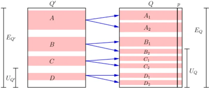
empty. Figure 2 illustrates this notion.
Our first lemma, which we state without proof, simply states that as we include more properties in a truth table, the support cannot increase.
Lemma 3.1. If Qand Q0 are two truth tables with Q ⊂ Q0, thenσ(Q, b)≥σ(Q0, b).
The next lemma establishes the anti-monotonicity of bal-ance and support.
Lemma 3.2. If a truth table Q has balance b and sup-ports, then every truth tableQ0⊆Qsuch that|Q0|
=|Q|−1
has balanceband supports.
Q Q0 UQ0 EQ0 UQ EQ B C D A1 A2 B1 B2 C1 C2 D1 p D2 A
Figure 2: An example of a truth table Q0 with k− 1 properties and a truth table Q that contains an additional property p.
Figure 2 illustrates the ideas used in the proof. In this figure, vertical lines denote the extent of EQ0, EQ, UQ0,
and UQ. Shaded rectangles denote object sets. The figure
indicates that the object set
1. A∈EQ0−UQ0 is the parent ofA1, A2∈EQ−UQ,
2. B ∈EQ0 −UQ0 is the parent of B1 ∈ EQ−UQ and
B2∈UQ,
3. C∈EQ0−UQ0 is the parent ofC1, C2∈UQ, and
4. D∈UQ0 is the parent ofD1, D2∈UQ.
Proof. Let Q have k properties. By the definition of
support, |UQ| ≤ (1−s)2k. LetQ0 be a truth table such
that Q0 ⊆Qand |Q0|
=k−1. Consider any object set S inEQ0. There are three cases to consider:
(i) S∈UQ0(e.g., object setDin Figure 2): Since|S1|,|S2| ≤
|S| ≤bn, bothS1 andS2 are elements ofUQ.
(ii) S∈EQ0−UQ0 and bothS1 and S2 have size at least
bn(e.g., object setAin Figure 2): bothS1andS2are
elements ofEQ−UQ.
(iii) S ∈ EQ0−UQ0 and at least one of S1 or S2 has size
less thanbn(e.g., object setC in Figure 2).
Let xbe the number of object sets inUQ whose parent is
in EQ0−UQ0. The number of such parents is at most x.
Therefore, we have the following inequality: |UQ|= 2|UQ0|+x≤(1−s)2k.
Since x ≥ 0, we have |UQ0| ≤ (1−s)2k−1, which implies
thatQ0 has balanceband supports.
Note that if we had defined the balance of a truth tableQ asβ(Q) = minS∈EQ|S|
n/2k , this lemma may not hold. In
partic-ular, if the truth tableQ0in the proof hasσ(Q0, b)< s, any object setS∈UQ0 has size less thanbn/2k−1. However, one
of the object set S partitions into in EQ may have size at
leastbn/2k, thus enablingσ(Q, b) to be at leasts, violating the desired anti-monotonicity.
Lemma 3.3. LetQbe a truth table withkproperties, bal-anceb and support1. If there is at least one object set in
EQ with size less than2bn, then every truth tableQ0 ⊃Q
with balancebhas support strictly less than1.
Proof. LetSbe the offending object set inEQ. LetQ0⊃
Qbe a truth table withk+ 1 properties. The object setSis the parent of two object setsS1 andS2inEQ0. Since|S|<
2bn, at least one of S1 or S2 must have size less than bn,
which implies thatQ0 does not have support 1.
The previous lemma implies a stronger form of the anti-monotone property guaranteed by Lemma 3.2 for the case when the support is 1.
Corollary 3.4. IfQ is a truth table withk properties, balanceband support1, then every sub-truth table ofQwith
k−1properties has balance2band support1.
We can generalise the previous lemma to all values of sup-ports.
Lemma 3.5. Let Q be a truth table with balance b and supports. Suppose that there arelQ object sets inEQwith
size at leastbn and2bnand that there arevQobject sets in
EQ with size at least 2bn. If lQ+vQ < s2k+1, then every
truth table that contains the properties inQand has balance
bhas support strictly less thans.
Proof. Consider any truth table Q0 ⊃ Q with k+ 1 properties. Consider any of thelQ−vQ object sets inEQ
with size betweenbn and 2bn; each such object set is the parent of at most one object set inEQ0 whose size is at least
bn. An example is object setB in Figure 2. Each of thevQ
object sets inEQwith size at least 2bn is the parent of at
most two object sets inEQ0 whose size is at leastbn. All
other object sets inEQare elements ofUQ. Hence, they are
parents of object sets inUQ0. ThereforeEQ0 can contain at
mostlQ−vQ+ 2vQ=lQ+vQobject sets with size at least
bn. IflQ+vQ< s2k+1, thenσ(Q0, b)< s.
4.
MINING TRUTH TABLES
Since our balance and support constraints apply anti-monotonically (see Lemma 3.2), we present a simple level-wise algorithm, a la Apriori, to find all truth tables in a relation that satisfy given balance and support constraints. For each k ≥ 1, given all truth tables with k properties, we construct candidate truth tables withk+ 1 properties. We use the heuristic of generating candidate truth tables at level k by merging two balanced and supported truth ta-bles at level k−1 such that they share k−2 properties in common [1] (we encapsulate this step in the
Generate-Candidatessubroutine, which is identical to the one in the Apriori algorithm [1]). For each candidate truth table T, we check if every sub-truth table of T with k properties satisfies the balance and support constraints. Finally, we perform one pass over the relation to compute the balance and support of each candidate truth table. We output only those candidates that satisfy these constraints.
Any truth tableQwithkproperties that satisfiesσ(Q, b)≥ smust contain at least s2k non-empty row subsets in EQ.
Since a trivial bound on the size ofEQ isn, the number of
objects inO, we see that no truth table can contain more thandlog(n/s)eproperties.
Algorithm 1FindTruthTables(O,P,R,b,s):
Input: A relationRrelating objects inOto properties inP, a balance threshold 0≤b≤1 and a support threshold 0≤s≤1.
Output: All truth tablesT suchσ(T, b)≥s. 1: T ← {p∈P |σ({p}, b)≥s}
2: whileTis not emptydo
3: forevery truth tableT ∈ T do
4: forevery truth tableT0⊆T,|T0|
=|T| −1do 5: if σ(T0, b)< sthen 6: DiscardT 7: end if 8: end for 9: Computeσ(T, b) 10: if σ(T, b)≥sthen 11: OutputT 12: InsertT intoT 13: end if 14: end for 15: T ←Generate-Candidates(T) 16: end while P1 P2 P3 o1 0 0 0 o2 1 0 1 o3 1 1 0 o4 0 1 1
Figure 3: Example dataset for illustrating relation-ships between truth tables and redescriptions.
In each outer loop, we efficiently computeσ(T, b) for ev-ery truth tableT in the current set of candidatesT, as fol-lows. Suppose we are currently processing candidates with k properties. Recall that for an object o∈O, oQdenotes
the binary vector with |T|elements given by the values of the properties inT ino. We consideroQto be a number in
binary notation. For each truth table T ∈ T, we maintain 2k+ 2 quantities:
(i) cT ,i,0 ≤i < 2k counts the number of objects o∈ O
such thatoT =i,
(ii) lT=|{cT ,i,0≤i <2k|cT ,i≥bn}|, i.e., the number of
object sets inET with size at leastbn, and
(iii) vT =|{cT ,i,0≤i <2k|cT ,i≥2bn}|, i.e., the number
of object sets inET with size at least 2bn.
As we read the properties contained in each object ofrom R, we compute oT and update the corresponding values.
AssumeoT =i. After incrementingcT ,i, we incrementlT if
cT ,i equalsbnor we incrementvT iscT ,i equals 2bn. After
we finish processingR, we can computeσ(T, b) aslT/n.
ComputingvT allows us to exploit Lemma 3.5 to prune
our search further. IflT +vT < s2k+1, then we know that
for any truth table T0 that contains the properties in T, σ(T0, b) < s. We can remove T from the list Tused to generate candidates for the next level.
5.
RELATIONS TO REDESCRIPTIONS
We now outline relationships between truth tables and re-descriptions. Redescriptions are a newly introduced class of data mining patterns [13] that establish similarity relation-ships between general boolean formulae.^P2 P1 equiv P2 ^P1 P1 P1 XOR P2 P2 ^P1^P2 P1^P2 P1P2 ^P1P2
FALSE
P1+^P2 P1+P2 ^P1+^P2 ^P1+P2
TRUE
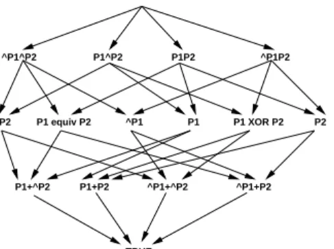
Figure 4: A relaxation lattice over expressions in-volving two boolean variables.
Consider as before relationR⊆O×P; adescriptoroverP is a boolean expression on a set of propertiesV ⊆P. Given a descriptore, we will denote the set of objects for whiche is true (for a presumedR) byO(e). Two descriptorse1and
e2 defined over (resp.) V1 and V2 are distinct (denoted as
e1 6=e2), if one of the following holds: (i)V1 6=V2, or (ii)
there exists someRfor whichO(e1)6=O(e2). Note that this
condition rules out tautologies. For instance, the descriptors P1∩P2andP1−(P1−P2) are not distinct. A descriptore0
is aredescriptionofeif and only ife6=e0andO(e) =O(e0) holds for the givenR. In this case, we say thate⇔e0.
Observe that redescriptions subsume association rules in expressive power, since they generalize implications to equiv-alences. Every (100% confident) association rule can be re-stated as a redescription but not the reverse. For instance, the association ruleP1 →P2 (i.e., objects that have
prop-ertyP1also have propertyP2) is equivalent to the
redescrip-tionP1 ⇔P1∩P2 (i.e., objects that have property P1 are
the same as the objects that have both of propertiesP1and
P2).
Consider the artificial dataset shown in Figure 3 with four objects and three properties. Let us attempt to identify re-descriptions by enumerating all possible boolean expressions and, for simplicity, focus on only the two propertiesP1 and
P2. We know that two properties can induce 22 2
boolean expressions, which can be arranged in a relaxation lattice as shown in Fig. 4. In this lattice, we have an arrow from expression e1 to e2 iff e1 entails e2, i.e., iff ¬e1 ∨ e2 is a
tautology; we then say thate2is arelaxationofe1. Observe
that the relaxation relation is dataset-agnostic, whereas re-descriptions are not.
To mine redescriptions between expressions in Fig. 4, we assess if two or more of them induce the same object set. The reader can verify that, in fact, all 16 boolean expres-sions induce all possible 24 = 16 subsets of objects from Fig. 3, and hence there are no possible redescriptions in this dataset! This is because the two propertiesP1 andP2form
a truth table over the given objects.
We have thus shown, by means of an example, that a dataset that induces a truth table of support 1 (i.e., all bit-wise combinations are present) cannot induce redescriptions. The reader can verify that the balance parameter is not rele-vant for this relationship, as long as it is non-zero. We hence state the following (for a proof, see [11]):
Theorem 5.1. Let R ⊆ O×P be a relation between n
objects and m properties such that each of the possible2m
presence/absence combination of properties is observed inR. Let e be a descriptor overP. Thene has no redescription with any other descriptor defined over P.
To make the analogy more concrete, consider what hap-pens when we delete a single row from the dataset in Fig. 3, say the last row. When we delete rowo4, we see noticeable
changes in the landscape of redescription terrains (Figure 5 (left)). Now, not only do redescriptions happen, every pos-sible expression has a redescription! For instance, we obtain the redescriptionP1⇔P1+P2where the + symbol denotes
logical OR, or union. This redescription states that objects that have eitherP1 orP2(or both) are the same as objects
that haveP1. Observe that this results because we deleted
objecto4, the only object that hadP2but notP1. Similarly,
the redescriptionP1 ANDP2⇔P1 XORP2 results for the
same row deletion.
Theorem 5.2. Let R ⊆ O×P be a relation between n
objects and m properties such that at least one of the pos-sible 2m presence/absence combination of properties is not observed in R. Then every descriptor e over P has a re-descriptione06=e.
As more rows are deleted, we observe a progressive, sys-tematic, halving of the number of equivalence classes, as depicted in Figure 5 (middle, right).
Corollary 5.3. Let R ⊆ O×P be a relation between
n objects and m properties such that κ of the possible 2m
presence/absence combination of properties are not observed in R. Then every descriptor e over P has 2κ−1distinct redescriptions.
The net effect of the above results culminates in:
Theorem 5.4. (Dichotomy Law) Let R ⊆ O×P be a relation between n objects and m properties. Then either no expression e over P has a distinct redescription or all expressionse overP have distinct redescriptions.
(Although this theorem makes mining redescriptions ap-pear to be a fruitless exercise, the task becomes interesting if we restrict the form of e, e.g., to be monotone, or to be conjunctions, in which case the dichotomy law doesn’t hold, and the problem becomes non-trivial.) Returning to the example in Fig. 3, it is clear that, since every pair of columns induces a truth table, no redescriptions are possi-ble between P1 and P2, between P2 and P3, and between
P1 and P3. Nevertheless, there are redescriptions possible
between all three of them, since the set of three properties doesnot induce a truth table. For instance, the redescrip-tion P1∪P2 ⇔ P2∪P3 holds. This suggests that the
al-gorithm presented in this paper can be combined with the one described in [11] (that identifies redescription terrains) to fruitfully complement each other. The truth table miner can suggest to the redescription miner to directly proceed to expressions involving all three variables. Similarly, the re-description miner can suggest to the truth table miner that it is not worthwhile to proceed beyond level 2 in its levelwise search. This helps create a dual mining strategy to model either class of patterns. This approach is akin to algorithms such as Pincer search [8] that maintain two borders of pat-terns.
FALSE ^F2 F1 equiv F2 ^F1 F1 F1 XOR F2 F2 ^F1^F2 F1^F2 F1F2 ^F1F2 F1+^F2 TRUE ^F1+^F2 ^F1+F2 F1+F2 FALSE ^F2 F1 equiv F2 ^F1 F1 F1 XOR F2 F2 ^F1^F2 F1^F2 F1F2 ^F1F2 F1+^F2 TRUE ^F1+^F2 ^F1+F2 F1+F2 FALSE ^F2 F1 equiv F2 ^F1 F1 F1 XOR F2 F2 ^F1^F2 F1^F2 F1F2 ^F1F2 F1+^F2 TRUE ^F1+^F2 ^F1+F2 F1+F2
Figure 5: Redescription terrains form as rows are successively deleted from a truth table. (left) one row deletion, (middle) two row deletions, and (right) three row deletions. The redescription terrains displayed as closed curves are based on the data shown in Fig. 3 restricted to the first two columns F1, F2. The first
figure uses rowso1, o2, o3. The middle figure uses rowso1, o2. The right figure uses o1.
6.
APPLICATIONS
We present our results in three parts. First, we perform a comprehensive analysis of the ability of our algorithm to recover a truth table planted in a random binary matrix. Next, we discuss how our method unravels complex features of the network regulating gene expression in a cell. Finally, we mine voting patterns of U.S. senators to detect patterns of independence among them. Due to space constraints, we chose to highlight different aspects of our algorithm in these case studies: (i) synthetic data: scalability and the effect of dataset characteristics on algorithm running time; (ii) gene expression regulation: effect of balance and support thresh-olds on running time as well as truthy nuggets of discovered knowledge; (iii) senatorial voting patterns: statistical inde-pendence of properties in a truth table and domain-specific insights.
6.1
Synthetic Data
To systematically study the ability of our algorithm to find truth tables, we planted them in random binary matri-ces and tested the ability of our algorithm to discover the planted truth tables. We first describe our protocol in detail. We constructed random matrices based on three parameters k, r, andp. Note that these values are parameters for the simulation and not for the truth table mining algorithm. For each such triple, we perform the following steps:
1. Generate a binary matrixM withk columns and 2k rows.
2. Select a random integerr, where 2≤r≤k, and plant a truth table with r columns in M. The truth table has balance 1/2r and support 1. The r columns are interspersed randomly among the columns onM. 3. Set every element ofM not belonging to the truth
ta-ble to be a 1 with probabilitypand a 0 with probability 1−p.
4. Execute the truth table finding algorithm onM with b= 1/2r ands= 1.
We executed these steps 10,000 times for the following choices of parameters: k∈ {5,10,15,20,25}, five random values of r, and 11 values of pbetween 0 and 1 in increments of 0.1 For every (k, r, p) triple, we computed the average running time of our algorithm.
Our algorithm successfully recovered the planted truth table in every case. Therefore, in this section, we focus on
presenting various slices of the three-dimensional function defined by the k, r, p and t(denoting time) values. A key feature of these results is the symmetric dependence of the running time onp. Unlike itemset and association rule min-ing algorithms, whose runnmin-ing time increases with p, the performance of our truth table mining algorithm is worst forp= 0.5 and symmetrically reduces around this value.
Dependence on
p.
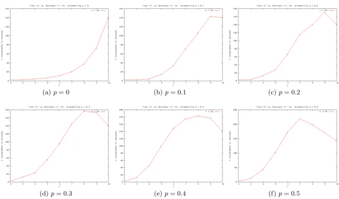
Figure 6 displays how the running timeof our algorithm depends on the probabilityp. Each plot in the figure corresponds to a fixed value ofk. Each curve in a plot represents a fixed value ofr. Due to lack of space, we only plot values for k= 5 andk = 10. As expected, these plots are symmetric around the linep= 0.5. For all values ofk, the plot forr=k is a nearly horizontal line, which is to be expected since the truth table spans the entire matrix. Observe that in Figure 6(a) (wherek= 5), the curve for any value of r dominates the curves for all smaller values ofr. However, the behaviour is subtly different fork = 10 (Figure 6(b)). Whereas the curves for the range r = 2 to r = 7 follow this trend, none of the curves for r = 7,8,9, and 10 dominate each other. In particular, focus onr= 7 and r = 8. The curve for r = 7 dominates the curve for r = 8 for values of p approximately between 0.4 and 0.6. We further examine this apparent discrepancy below.
Dependence on
k.
Next, we examined how the runningtime varied with the number of columnskin the matrix, for fixed values ofp. We fixedk= 10, since this case exemplifies higher values ofkas well. Each plot in Figure 7 corresponds to a fixed value of p. We show the plots only forp≤0.5, because of symmetry. Consider Figure 7(a), wherep = 0. The larger the value of the size of the planted truth table (r), the greater the running time of the algorithm. Now consider the other extremep= 0.5 (Figure 7(f)). The running time has an inflection point atr= 7.
The running time of our algorithm on these synthetic datasets is primarily composed of two factors: 1. the time taken to discover the planted truth table and 2. the time spent in processing properties that do not belong to the planted truth table. The first component monotonically in-creases withr whereas the second component is influenced both byk−rand byp. The second component is not mono-tonic inr. In this case, the contribution of the second
com-(a)k= 5 (b)k= 10
Figure 6: Plots of running time (t) vs. k for fixed values of the probabilityp.
(a)p= 0 (b)p= 0.1 (c)p= 0.2
(d)p= 0.3 (e)p= 0.4 (f)p= 0.5
ponent to the running time starts decreasing dramatically forr≥7. The exact relationship between these components is worth further study.
Scalability.
Finally, we examined the scalability of oural-gorithm as dataset size increases. Recall that askincreases linearly from 5 to 20, the number of rows in the matrix in-creases exponentially ink. We focus on smaller values ofr (in particular two and three) so as to make the dependence of running time on dataset size more explicit. Figure 8(a) and (b) show the dependence on running time forr= 2 and values of p= 0.1 andp = 0.5, respectively. The y-axis in these figures is on a logarithmic scale. Observe thatphas negligible effect and that the running time mirrors the expo-nential growth in dataset size. Figure 8(c) and (d) show the dependence on running time forr= 3 and values ofp= 0.1 and p = 0.5, respectively. Although we observe the same trends in each of the last two graphs, note that forr= 3 and p= 0.5, the algorithm runs an order of magnitude slower (the range of the y-axis in Figure 8(c) is [0,104] while the range in Figure 8(c) is [0,105]). This observation reinforces
the breakdown of running time into two components, in par-ticular the role played by sparsity.
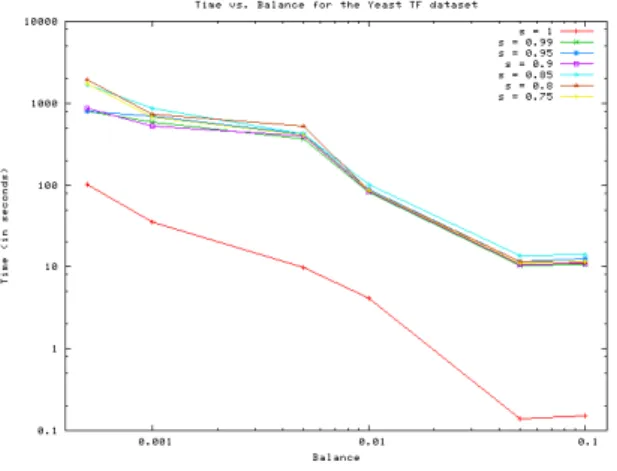
(a) Running timetvs. balance thresholdbfor fixed values of the support thresholds.
(b) Running timetvs. support thresholdsfor fixed values of the balance thresholdb.
Figure 9: Performance of the truth table mining algorithm on theS. cerevisiae TF dataset.
6.2
Combinatorial Regulatory Networks
Gene expression in eukaryotic cells is controlled by the combinatorial interaction of transcription factors (TFs) and their binding motifs in DNA [2]. TFs often operate hi-erarchically: master regulators govern gene expression in multiple conditions, and act combinatorially with tissue- or condition-specific TFs to modulate gene expression. Truth tables representing TFs and the genes they regulate promise to capture the complexity of combinatorial regulation in eu-karyotic cells.To investigate this possibility, we analyzed a dataset of transcriptional regulation inS. cerevisiae[7] (baker’s yeast). The dataset is a binary matrix whose columns represent 112 transcription factors and whose rows represent 4603 genes inS. cerevisiae; the matrix contains 12804 non-zero entries. A matrix entry contains a one if a ChIP-on-chip experiment indicates that the transcription factor binds to the promoter of the gene with a p-value at most 0.001. Although ChIP-on-chip data is noisy and significant effort may be needed to clean it up, the analysis we present next demonstrates that truth tables in such datasets can provide useful biological insights.
We ran our truth table finding algorithm on this dataset for balance values of 0.1,0.05,0.01,0.005,0.001, and 0.0005 and support values of 1,0.99,0.95,0.9,0.85,0.8, and 0.75. Figure 9(a) displays on a log-log plot how the running time of the algorithm depends on the balance threshold we use. Each curve is this plot corresponds to a fixed value of sup-port. We see that the logarithm of the running time is in-versely proportional to the logarithm of the balance, for any given value of support. The plots also indicate that the case s= 1 requires less effort from the algorithm than values of support less than 1. Figure 9(a) displays on a log-log plot how the running time of the algorithm depends on the sup-port threshold we use. As long as the supsup-port is less than 1, changing it does not have an adverse affect on the running time of the algorithm.
We mined truth tables by executing our algorithm on this data withb= 0.001 ands= 0.75. Our algorithm computed 6105 two-TF, 60570 three-TF, 6298 four-TF, and nine five-TF truth tables. We further examined the five-five-TF truth ta-bles. One truth table includes the TFs CIN5, PHD1, RAP1, SKN7, and SWI4. The other eight truth tables involved various combinations of seven TFs: ACE2, FKH2, MBP1, NDD1, SKN7, SWI4, and SWI6. Note that the two sets share the TFs SKN7 and SWI4.
We first discuss the truth table involving RAP1, PHD1, CIN5, SWI4, and SKN7 in detail. PHD1 and SKN7 are TFs that regulate different aspects of cell growth. SWI4 is a key TF regulating the G1/S transition of the mitotic cell cycle. RAP1 is involved in chromatin silencing. SKN7 responds to different types of osmotic and oxidative stress while CIN5 is responsible for inducing the cell’s response to drugs. The presence of all five TFs in a truth table suggests an intricate process of regulation that governs how the cell responds to external agents of stress potentially by shutting down the cell cycle and controlling its growth.
The truth tables that include ACE2, FKH2, MBP1, NDD1, SKN7, SWI4, and SWI6 shed light on other aspects of cellu-lar growth and cell cycle control. FKH2 and NDD1 regulate G2/M-specific transcription in the mitotic cell cycle whereas ACE2 controls G1-specific transcription. MBP1 regulates progression through the cell cycle and is involved in DNA
(a)r= 2, p= 0.1 (b)r= 2, p= 0.5 (c)r= 3, p= 0.1 (d)r= 3, p= 0.5
Figure 8: Plots of running time (t) vs. k for fixed values of the probabilityp.
replication. The shared membership of SKN7 and SWI4 in both groups of truth tables leaves open the possibility that as we discover more relationships between TFs and target genes, we may detect truth tables involving all ten TFs, thus coming closer to a more complete picture of transcriptional regulation in conditions of external stress.
6.3
Voting Dimensions of U.S. Senators
We also applied our truth table finding algorithm to voting patterns of the U.S. Senate. In particular, we obtained the roll call votes for first session of the 102nd Congress in 1991 from the Thomas database at the Library of Congress. This data contains the votes of 101 senators on 280 bills. A roll call vote guarantees that every senator’s vote is recorded. We considered a “yes” vote to be a 1 and “no” vote or an abstension to be a 0.When we used b= 0.01, and s = 1, all truth tables we mined had five or fewer bills. We used theχ2 test to assess the independence of the bills in a truth table. Of the 60481 five-bill truth tables we found, 17976 were significant at the 0.01 level. We selected one of these significant truth tables at random to qualitatively assess the independence of the bills in it. The truth table we chose contained the bills
1 Nunn Resolution Re: Persian Gulf - S.J. Res. 1; A joint resolution regarding United States policy to reverse Iraq’s occupation of Kuwait.
16 Dodd Amdt. No. 11; To amend the Export-Import Bank Act of 1945
39 Motion To Table S. Amdt. 59; To eliminate or reduce certain appropriations.
133 Byrd amdt.; To provide for an equalization in certain rates of pay, to apply the honoria ban and the provi-sions of title V of the Ethics in Government Act of 1978 to Senators and officers and employees of the Senate, and for other purposes
267 Motion To Table D’Amato Amendment No. 1405; To amend the Harmonized Tariff Schedule of the United States to clarify the classification of certain motor ve-hicles
These bills span diverse aspects of the political landscape: war, banking, pork, ethics, and trade.
We also counted the frequency of occurrence of each bill in significant truth tables. Interestingly, the five most fre-quent bills—39, 66, 97, 267, and 279—form a truth table themselves! Notice that we have already encountered bills 39 and 267. The subjects of the other three bills are the following:
66 Moynihan Amdt. No. 249; To amend the Ethics in Government Act of 1978 to apply the limitations on outside earned income to unearned income.
97 Motion To Table Amdt. No. 358; To eliminate lan-guage which lowers the Federal share payable for cer-tain projects
279 Conference Report; Comprehensive Deposit Insurance Reform and Taxpayer Protection Act of 1991
In addition to war (bill 39) and trade (bill 267), these bills pertain to ethics, pork, and insurance reform. Such patterns shed direct light on the weighty deliberations that occupied the members of the 102nd Congress.
7.
RELATED WORK
As stated earlier, truth tables form the anti-pattern to many concepts studied by other researchers. Brin et al. [16] were one of the first groups to find correlated sets of (bi-nary) attributes using theχ2significance test. The TAPER
algorithm [21] uses the Pearsons correlation metric instead; this work employs a upper bound on the correlation coef-ficient (for binary variables) to expose monotonicity con-straints [21] that are useful for conducting all-pairs queries. Truth tables withkproperties, balanceb1/2kc, and sup-port 1 can be viewed as a special case of dense itemsets (de-fined in [15]) where the density is 50%. Observe, however, that, the density is of a particular nature and is more restric-tive than the definition given by Seppanen and Mannila [15]. In particular, the form of density captured by a truth table obeys anti-monotonicity constraints without defining it as a statistic over densities of all its constituent sub-truth tables (as is done with the definition of weak density [15]). In gen-eral, the sparsity constraints of truth tables can be viewed as a sophisticated intersection statistic [14] over all (conjunc-tive) boolean expressions over the truth table’s columns.
Truth tables are inherently also related to approaches that seek to quantify independence in binary datasets, e.g., Pavlov et al. [12] (whose end goal is to approximate answers to complex queries) and those that assess the dimensional-ity of the underlying dataset, e.g., Tatti et al. [17] by count-ing the number of independent columns. In fact, our work can be generalized into yielding graphical models for binary data [18]. One of the critical issues in building such models is identifying subsets of variables that induce conditional in-dependence constraints. To support such analyses, we can generalise our definition of truth tables toconditional truth tablesi.e., a truth table that surfaces only in a subset of the given data.
The partition of the rows of a truth table into distinct blocks with sufficient balance each is reminiscent of the work by Gionis et al. [5] that aims to identify subsets of rows and columns with a certain level of sparsity. Viewed in light of this work, a truth table is a patchwork of combinatorial rect-angles each with a characteristic level of sparsity. However,
as mentioned earlier, by exploiting properties that are satis-fied by truth tables (but not combinatorial tiles in general), we are able to design effective algorithms.
8.
DISCUSSION
We have formulated the novel data mining problem of finding truth tables in a binary matrix. In the continuum of informative patterns, truth tables reside at the end op-posite that where itemsets and association rules lie, since truth tables represent properties that have no depenency patterns between them. The levelwise nature of the pro-posed mining algorithm means that we can employ many optimizations originally defined forApriori-like algorithms, such as bounding the number of possible candidate patterns at a certain level based on the number of frequent patterns at the level below it [4].
The notion of truth tables displaying 50% sparsity in a characteristic manner deserves further study. For instance, the theoretical question of feasibility of identifying truth ta-bles can be posed under given distributional assumptions (e.g., a Zipf distribution of the 0-1 data). We also intend to explore further the relationships between truth table min-ing and redescription minmin-ing toward designmin-ing dual-minmin-ing approaches.
9.
REFERENCES
[1] R. Agrawal and R. Srikant. Fast Algorithms for Mining Association Rules in Large Databases. In
Proceedings of the 20th International Conference on Very Large Data Bases (VLDB’94), pages 487–499, Sep 1994.
[2] L. O. Barrera and B. Ren. The transcriptional regulatory code of eukaryotic cells–insights from genome-wide analysis of chromatin organization and transcription factor binding.Curr Opin Cell Biol, 18(3):291–8, 2006.
[3] J.B. Fitzgerald, B. Schoeberl, U.B. Nielsen, and P.K. Sorger. Systems Biology and Combination Therapy in the Quest for Clinical Efficacy.Nature Chemical Biology, Vol. 2(9):458–466, Sep 2006.
[4] F. Geerts, B. Goethals, and J.V.D. Bussche. Tight Upper Bounds on the Number of Candidate Patterns.
ACM Transactions on Database Systems, Vol. 30(2):pages 333–363, June 2005.
[5] A. Gionis, H. Mannila, and J.K. Seppanen. Geometric and Combinatorial Tiles in 0-1 Data. InProceedings of the 8th European Conference on Principles and Practice of Knowledge Discovery in Databases (PKDD’04), pages 173–184, 2004.
[6] K. Goldberg, T. Roeder, D. Gupta, and C. Perkins. Eigentaste: A Constant Time Collaborative Filtering Algorithm.Information Retrieval, Vol. 4(2):pages 133–151, July 2001.
[7] Tong Ihn Lee, Nicola J. Rinaldi, Francois Robert, Duncan T. Odom, Ziv Bar-Joseph, Georg K. Gerber, Nancy M. Hannett, Christopher T. Harbison, Craig M. Thompson, Itamar Simon, Julia Zeitlinger, Ezra G. Jennings, Heather L. Murray, D. Benjamin Gordon, Bing Ren, John J. Wyrick, Jean-Bosco Tagne, Thomas L. Volkert, Ernest Fraenkel, David K. Gifford, and Richard A. Young. Transcriptional
Regulatory Networks in Saccharomyces cerevisiae.
Science, 298(5594):799–804, 2002.
[8] D.-I. Lin and Z.M. Kedem. Pincer-Search: An Efficient Algorithm for Discovering the Maximum Frequent Set.IEEE Transactions on Knowledge and Data Engineering, Vol. 14(3):553–566, 2002.
[9] S.C. Madeira and A.L. Oliveira. Biclustering Algorithms for Biological Data Analysis: A Survey.
IEEE/ACM Transactions on Computational Biology and Bioinformatics, Vol. 1(1):24–45, Jan 2004. [10] M. Natarajan, K.-M. Lin, R.C. Hsueh, P.C. Sternweis,
and R. Ranganathan. A Global Analysis of Cross-talk in a Mammalian Cellular Signaling Network.Nature Cell Biology, Vol. 8(6):571–580, June 2006.
[11] L. Parida and N. Ramakrishnan. Redescription Mining: Structure Theory and Algorithms. Technical report, Feb 2005.
[12] D. Pavlov, H. Mannila, and P. Smyth. Beyond Independence: Probabilistic Models for Query Approximation on Binary Transaction Data.IEEE Transactions on Knowledge and Data Engineering, Vol. 15(6):pages 149–1421, 2003.
[13] N. Ramakrishnan, D. Kumar, B. Mishra, M. Potts, and R.F. Helm. Turning CARTwheels: An
Alternating Algorithm for Mining Redescriptions. In
Proceedings of the Tenth ACM SIGKDD International Conference on Knowledge Discovery and Data Mining (KDD’04), pages 266–275, Aug 2004.
[14] J.K. Seppanen.Using and Extending Itemsets in Data Mining. PhD thesis, 2006.
[15] J.K. Seppanen and H. Mannila. Dense Itemsets. In
Proceedings of the Tenth ACM SIGKDD International Conference on Knowledge Discovery and Data Mining (KDD’04), pages 683–688, Aug 2004.
[16] C. Silverstein, S. Brin, and R. Motwani. Beyond Market Baskets: Generalizing Association Rules to Dependence Rules.Data Mining and Knowledge Discovery, Vol. 2(1):pages 39–68, 1998.
[17] N. Tatti, T. Mielikainen, A. Gionis, and H. Mannila. What is the Dimension of your Binary Data? In
Proceedings of the 6th IEEE International Conference on Data Mining (ICDM’06), pages 603–612, 2006. [18] J.L. Tuegels and J.V. Horebeek. Generalized
Graphical Models for Discrete Data.Statistics and Probability Letters, Vol. 38:41–47, May 1998. [19] List of newspeak words. Wikipedia. http://en.
wikipedia.org/wiki/List of Newspeak words #Bellyfeel.
[20] Truthiness. Wikipedia. http://en.wikipedia.org/wiki/ Truthiness.
[21] H. Xiong, S. Shekhar, P.-N. Tan, and V. Kumar. TAPER: A Two-Step Approach for All-Strong-Pairs Correlation Query in Large Databases.IEEE Transactions on Knowledge and Data Engineering, Vol. 18(4):pages 493–508, 2006.
[22] M.J. Zaki and N. Ramakrishnan. Reasoning about Sets using Redescription Mining. InProceedings of the Eleventh ACM SIGKDD International Conference on Knowledge Discovery and Data Mining (KDD’05), pages 364–373, Aug 2005.