A Multivariate Framework for Variable Selection and Identification of Biomarkers in High-Dimensional Omics Data

for Variable Selection and Identification of Biomarkers

in High-Dimensional Omics Data

Von der Fakultät für Mathematik und Informatik der Universität Leipzig

angenommene

D I S S E R T A T I O N

zur Erlangung des akademischen Grades

DOCTOR RERUM NATURALIUM

im Fachgebiet Informatik

vorgelegt

von M.Sc. Verena Zuber

geboren am 6. Juni 1983 in Donauwörth

Die Annahme der Dissertation wurde empfohlen von 1. Professor Dr. Jörg Rahnenführer (Dortmund)

2. Professor Dr. Peter F. Stadler (Leipzig)

Die Verleihung des akademischen Grades erfolgt mit Bestehen

Mein größter Dank geht an Korbinian Strimmer für die ausgezeichnete Betreuung. Im Besonderen möchte ich mich vielmals bedanken, dass seine Tür jederzeit für jegliche erdenkliche Frage offen stand. Nicht vergessen möchte ich zudem die äußerst hilfreichen Anregungen und Förderung zum kreativen und selbstständigen Arbeiten.

Darüber hinaus geht mein Dank an Professor Peter Stadler und an Pro-fessor Jörg Rahnenführer für die Korrektur der Arbeit.

Moreover, a huge "dankeschön" goes to my research group and its visi-tors for support, discussion, and advice. Thank you Bernd, Carsten, Miika, and Sebastian. Des Weiteren möchte ich meinen Kollegen am IMISE danken. Insbesondere geht mein Dank an Professor Markus Löffler für die Unter-stützung, Cornelia Will für die aufbauenden Worte, Dirk Hasenclever für seine statistische Expertise, Holger Kirsten und Peter Ahnert für den biolo-gischen Rat und Katja Rösch für den mathematischen Rat.

Meinen Eltern möchte ich danken für ihre anhaltende Unterstützung. Finally, big hugs to Deb and Yasmine for their support, advice, good vibes, and enthusiasm for science.

Und zu guter Letzt ein großes Dankeschön an den wunderschönen Kater Justus, der so lieb war, sein Fell für den Umschlag photographieren zu lassen, und natürlich an Ben, den stolzen Katzen-Besitzer.

In this thesis, we address the identification of biomarkers in high-dimensional omics data. The identification of valid biomarkers is especially relevant for personalized medicine that depends on accurate prediction rules. Moreover, biomarkers elucidate the provenance of disease, or molecular changes related to disease. From a statistical point of view the identification of biomarkers is best cast as variable selection. In particular, we refer to variables as the molecular attributes under investigation, e.g. genes, ge-netic variation, or metabolites; and we refer to observations as the specific samples whose attributes we investigate, e.g. patients and controls. Vari-able selection in high-dimensional omics data is a complicated challenge due to the characteristic structure of omics data. For one, omics data is high-dimensional, comprising cellular information in unprecedented details. Moreover, there is an intricate correlation structure among the variables due to e.g internal cellular regulation, or external, latent factors. Variable selection for uncorrelated data is well established. In contrast, there is no consensus on how to approach variable selection under correlation.

Here, we introduce a multivariate framework for variable selection that ex-plicitly accounts for the correlation among markers. In particular, we present two novel quantities for variable importance: the correlation-adjusted t

(CAT) score for classification, and the correlation-adjusted (marginal) correla-tion (CAR) score for regression. The CAT score is defined as the Mahalanobis-decorrelatedt-score vector, and the CAR score as the Mahalanobis-decorre-lated correlation between the predictor variables and the outcome. We derive the CAT and CAR score from a predictive point of view in linear discriminant analysis and regression; both quantities assess the weight of a decorrelated and standardized variable on the prediction rule. Furthermore, we discuss properties of both scores and relations to established quantities. Above all, the CAT score decomposes Hotelling’s T2 and the CAR score the proportion of variance explained. Notably, the decomposition of total variance into explained and unexplained variance in the linear model can be rewritten in terms of CAR scores.

To render our approach applicable on high-dimensional omics data we de-vise an efficient algorithm for shrinkage estimates of the CAT and CAR score. Subsequently, we conduct extensive simulation studies to investigate the performance of our novel approaches in ranking and prediction under correlation. Here, CAT and CAR scores consistently improve over marginal approaches in terms of more true positives selected and a lower model error. Finally, we illustrate the application of CAT and CAR score on real omics data. In particular, we analyze genomics, transcriptomics, and metabolomics data. We ascertain that CAT and CAR score are competitive or outperform state of the art techniques in terms of true positives detected and prediction error.

1 Introduction 1

1.1 Biomarkers and personalized medicine . . . 1

1.2 The search for biomarkers as statistical problem . . . 2

1.3 Contributions . . . 2

1.4 Outline . . . 3

2 Background 5 2.1 The biological background of omics data . . . 5

2.1.1 Genomics . . . 7

2.1.2 Transcriptomics . . . 9

2.1.3 Metabolomics . . . 10

2.2 The statistical background on variable selection . . . 11

2.2.1 Prediction . . . 12

2.2.2 Ranking . . . 16

3 Variable selection in classification 19 3.1 Prediction . . . 19

3.1.1 Discriminant analysis . . . 20

3.1.2 Logistic regression . . . 23

3.2 Variable ranking . . . 25

3.2.1 Quantities for variable importance . . . 25

3.2.2 Regularized estimates . . . 27

3.3 Decorrelation: The correlation-adjustedt-score . . . 30

3.3.1 Definition of the CAT score . . . 30

3.3.2 Derivation from linear discriminant analysis . . . 31

3.3.3 Properties of the CAT score . . . 33

3.3.4 Estimation . . . 35

3.4 Simulation studies . . . 36

3.4.1 Correlation scenarios . . . 36

3.4.2 Data generation . . . 38

3.4.3 Competing test statistics . . . 38

3.4.4 Comparison of variable rankings . . . 40

3.5 Summary . . . 41 vii

4 Variable selection in regression 43

4.1 Linear regression revisited . . . 44

4.1.1 The linear regression model and best linear predictor 44 4.1.2 The decomposition of variance . . . 46

4.1.3 Classical strategies for variable selection . . . 47

4.2 Prediction: Penalized regression . . . 49

4.3 Ranking variables by importance . . . 51

4.4 Decorrelation: The CAR score . . . 57

4.4.1 Definition of the CAR score . . . 57

4.4.2 Derivation from the best linear predictor . . . 58

4.4.3 The decomposition of variance in terms of CAR scores 59 4.4.4 The CAR score as quantity for variable importance . 60 4.4.5 More properties of the CAR score . . . 61

4.4.6 Estimation . . . 64

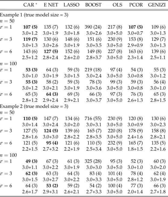
4.5 Simulation studies . . . 65

4.5.1 Design of the simulation study . . . 65

4.5.2 Results from the simulation study . . . 66

4.6 Comparison of CAT and CAR score . . . 70

4.7 Summary . . . 71

5 Computational issues 73 5.1 Special properties of the Mahalanobis transform . . . 73

5.2 Computationally efficient calculation . . . 74

5.3 On determining the model size . . . 76

5.3.1 Distribution under the null hypotheses of CAT and CAR score . . . 76

5.3.2 Penalized residual sum of squares . . . 79

5.3.3 Estimation of the prediction error by cross-validation 80 5.3.4 False (non) discovery rate . . . 81

6 Application to experimental data 83 6.1 Clinical data: Analysis of the diabetes data . . . 83

6.2 Genomics data: Analysis of SNP data . . . 85

6.2.1 GAW 17 unrelated data and preprocessing . . . 86

6.2.2 Relative performance of the rankings generated by the investigated methods . . . 87

6.3 Transcriptomics data . . . 93

6.3.1 Classification of prostate cancer . . . 93

6.3.2 Classification of lymphoma . . . 95

6.3.3 Classification of small round blue cell tumour . . . . 96

6.3.4 Classification of brain cancer . . . 97

6.3.5 Correlating gene-expression with age . . . 99

6.4 Metabolomics data . . . 101

A Notation 119 A.1 Symbols . . . 119 A.2 Abbreviations . . . 121

B Software 123

B.1 Implementation inR . . . 123 B.2 Step by step analysis

of the benchmark diabetes data . . . 125

Introduction

1.1

Biomarkers and personalized medicine

Personalized medicine is one of the great promises of modern clinical medicine (Hamburg and Collins, 2010). The aim is to tailor therapies to an individual patient, finding "the right drug for the right person" (Allison, 2008). Many diseases, including types of cancers, exhibit heterogeneous characteristics in clinical outcome or responsiveness to drug therapy. A correct diagnosis of such specific subtypes of cancer aids to administer the ideal targeted therapy. For example, scientists identified a molecular pattern in women suffering from breast cancer that can be used to quite accurately predict recurrence of cancer after surgery. This diagnostic test helps to decide whether the patient needs to undergo continuing chemotherapy (Paik et al., 2004). Personalized medicine reduces costs by improving the clinical success rate of the therapy prescribed (Woodcock, 2007) and thus can be beneficial for the patient as well as for the health care system. Moreover, pharmaceuti-cal companies are able to increase the efficiency of their drugs if they can exactly predict which patients respond to the drug. This has prompted some pharmaceutical companies to develop drug/diagnostic pairs (Allison, 2008).

The success of personalized medicine decisively depends on the accu-racy of the diagnosis (Hamburg and Collins, 2010). Thus, the discovery of precisebiomarkers for diseaseis essential. Over the last two decades biotech-nological inventions, like the microarray, sequencing technologies, or mass-spectrometry, have provided unprecedented information on biological and molecular processes. Such techniques enable comprehensive views on all constituents of the cell, ranging from the genetic code, to protein synthesis, and the metabolism. Derived from the Greek word for “all-encompassing”

omicshas been coined as a general term for this emerging data since it can literally comprise all constituents. For example, modern microarrays can measure the activity of all 25, 000 genes known in human. In particular, the microarray technology has stimulated the search for molecular biomarkers. See e.g the reference publications by Golub et al. (1999), Ramaswamy et al.

(2001), or Veer et al. (2002) that propagate molecular cancer diagnosis. Apart from prediction, biomarkers can also provide insight into the heterogeneity and molecular changes of disease states (Schilsky, 2010).

1.2

The search for biomarkers

as statistical problem

From a statistical point of view the discovery of biomarkers is best cast as variable selection. In particular, we refer to variables as the molecular attributes under investigation, e.g. genes, genetic variation, or metabolites; and we refer to observations as the specific samples whose attributes we investigate, e.g. patients and controls.

Variable selection in omics data poses an intricate challenge due to the characteristic data structure of omics data. First, omics data is high-dimensional, literally comprising all constituents. Unfortunately, the limita-tion in omics data is the sample size that has not expanded with the same speed as the dimension of variables. Second, certain processes and elements of the cell are interconnected in complex patterns due to e.g internal cellular regulation or external, latent factors influencing the cell. This results in anintricate correlation structureamong the variables. Variable selection for uncorrelated data is well established. In contrast, there is no consensus on how to approachvariable selection under correlation.

1.3

Contributions

This thesis illustrates our attempt to incorporate knowledge on the corre-lation structure into the selection of variables. Since omics data exhibit an intrinsic correlation structure among variables, we argue that it is beneficial to incorporate this information in the selection of variables. In particular, we propose two novel quantities for variable selection that explicitly model the correlation structure, the correlation-adjustedt(CAT) score in classification and the correlation-adjusted (marginal) correlation (CAR) score in linear regression.

To allow application of CAT and CAR scores in high-dimensional omics data we devise an efficient algorithm to derive estimates of CAT and CAR scores. Hence, we provide two highly competitive approaches for variable selection and biomarker identification in high-dimensional omics data. The CAT and CAR score are implemented in the publicly available packagesst andcarein the free statistical programming languageR (R Development Core Team, 2012).

We compare our approaches with other state-of-the-art techniques in extensive simulation studies, where both the CAT and the CAR score are

on par with or even outperform their competitors in terms of true positives selected and prediction error. Moreover, we illustrate the application of CAT and CAR score in high-dimensional omics data. We analyze the performance of CAT and CAR score in genomics, transcriptomics, and metabolomics data.

This thesis is based on the following publications:

• V. Zuber and K. Strimmer. 2009.Gene ranking and biomarker discovery under correlation.Bioinformatics 25 (20): 2700-2707

• V. Zuber and K. Strimmer. 2009. Correlation-adjusted t-scores in applica-tion to funcapplica-tional magnetic resonance imaging data. Proceedings of the 6th International Workshop on Computational Systems Biology, WCSB 2009 (June 10-12, 2009, Aarhus, Denmark). pp. 163-166.

• V. Zuber and K. Strimmer. 2011. High-Dimensional Regression and Variable Selection Using CAR Scores. Statistical Applications in Genetics and Molecular Biology 10: 34

• V. Zuber, P. Duarte Silva, and K. Strimmer. 2012. A novel algorithm for simultaneous SNP selection in high-dimensional genome-wide association studies. BMC Bioinformatics 13:284

1.4

Outline

This thesis is organized as follows. First, we illustrate background infor-mation on the scope of this thesis. Section2.1describes the biological back-ground of omics data, while Section2.2sketches the statistical background of variable selection. In particular, we distinguish between variable selection with respect to prediction or ranking. Then, Section3and Section4provide detailed information on strategies for variable selection in classification and linear regression, respectively. Both chapters share the same structure; in the beginning existing approaches to variable selection in prediction and ranking are discussed. Then, we present our novel quantities for variable selection, the CAT score is introduced in Section3.3, and the CAR score in Section4.4. Subsequently, we discuss the derivation, properties, connection to different established quantities, and strategies for estimation. To conclude, both chapters report results on extensive simulation studies.

In Section5we illustrate algorithmic details on the estimation of CAT and CAR scores. In particular, we highlight an efficient algorithm that allows to use our approaches even in the case of large dimensional omics data. Finally, Section 6reports comprehensive studies of real omics data. This includes genomics in Section6.2, transcriptomics in Section6.3, and metabolomics in Section6.4.

Background on omics data and

variable selection

This chapter provides introductory information on the scope of this thesis. First the biological background of omics data is provided to motivate the study of variable selection under correlation in statistics. Then, the basics of variable selection are established to introduce the elementary concepts of prediction and ranking.

2.1

The biological background of omics data

The last decade of biological science witnessed revolutionary biological dis-coveries and biotechnological inventions, that allow to investigate processes in the cell on new levels of accuracy.

It has been in the year 1953 that James D. Watson and Francis Crick described a structural model of the genetic code encoded in the deoxyri-bonucleic acid (DNA) by a helix model (Watson and Crick, 1953). This discovery was awarded the Nobel Prize in Physiology or Medicine. In 1958 Francis Crick reported the synthesis of proteins from DNA in two distinct phases: Transcription and translation (Crick (1958) and Crick (1970)). The DNA sequence, given by a specific sequence of nucleotides, is the most elementary part of life and the starting point of the genetic information flow. Genes constitute certain regions of the DNA. In thetranscription phase

DNA is recoded into complementary ribonucleic acid (RNA) that includes messenger RNA (mRNA), ribosomal RNA (rRNA), transfer RNA (tRNA) and micro RNA. The transcription of genes that encode proteins results into mRNA; thus, mRNA is the carrier of protein information that is synthesized in thetranslation phaseunder influence of rRNA and tRNA into proteins, the product of cells. See e.g. Pollard and Earnshaw (2007) for more detailed information of the protein synthesis. With the advent of blotting technolo-gies in the 1970’s it became possible to actually measure the mRNA level, also referred to as expression, of single genes in cells. Twenty years later,

microarrays have turned-over the perspective on how detailed processes in the cell can be observed as they allow to measure the expression of several thousands of genes at once. The development of high-throughput microar-rays was revolutionary since it captured not only the expression of single genes but the expression of the vast majority of all known genes. Thus, it became practicable to actually map the transcriptome, that is all mRNA constituents of the transcription phase.

Moreover, biotechnological inventions have changed the perspective on further components of the genetic information flow. Sequencing techniques allow to explore the genome, the entire genetic code. So far genomes of sev-eral species have been sequenced; most spectacular has been the sequencing of the human genome by the International Human Genome Sequencing Con-sortium (2001). Today also products of the translation phase are explored in great multiplicity and detail. Mass spectrometry and nuclear magnetic resonance spectroscopy provide insights into the proteome and metabolome, that is all proteins, respectively all metabolites in a cell.

Derived from the greek word “ome” referring to all constituents, “omics” describes the study of all constituents. Thus,omicshas become a synonym for the datasets produced by modern high-throughput technologies. Charac-teristic for omics data is for one the large size of observed variables, literally comprising all constituents, and only moderate numbers of observations. Hence, such data sets are described as “smalln, larged”, wherenrefers to the number of observations anddto the number of attributes investigated. Furthermore, there is an intrinsic correlation or dependence structure due to unobserved biological processes that influence the observed data, e.g internal cellular regulation, or external, latent factors. More detail on the respective dependence structures is provided in the following sections.

These decisive changes in data structure demanded new strategies for analysis. While standard statistic tools require that the number of observa-tions is larger than the dimension of variables, i.e. n > d, the new small

n, larged, setting of omics data triggered new innovations in statistics, in particular, regularized regression, the false discovery rate, and a rediscovery of Stein’s shrinkage estimates.

Before delving deeper into statistical modeling the next sections discuss in greater detail the most prominent examples for omics data that are used to discover biomarkers. Section6illustrates the analysis of high-dimensional omics data from the following levels in the protein-synthesis of a cell and beyond:

• Genomics: DNA sequence level

• Transcriptomics: (m)RNA level

2.1.1

Genomics

Genomics refers to the study of the genome of organisms which is encoded in the DNA. In humans, DNA segments are incorporated in two homolo-gous chromosomes, each inherited from a parent. The DNA information is represented by the four DNA bases or nucleotides: Adenin, thymin, gua-nine, and cytosine. Genotype is the term for DNA base pairs observed at a specific location. Specific DNA segments code genes or constitute noncoding-regions.

Genetic association studies focus on genetic variation that is captured by so called single nucleotid polymorphisms (SNPs). A SNP is defined as “a single base pair change that is variable across a certain fraction of the general population” (Foulkes, 2009). Association refers to the relationship of the observed genotype to a phenotype of interest. It is studied either in an hypothesis-driven way in candidate gene or fine mapping studies, where only small parts of the genome are considered, or in an exploratory style in genome-wide association studies (GWAS). GWAS have become feasible by the development of next-generation sequencing techniques that parallelize the sequencing process and thus allow to measure vast parts of the genome (Schuster, 2008). The most prominent sequencing technologies are the 454 pyrosequencer, the Ilumina, and SOLiD sequencing. For detailed information of theses high-throughput sequencing techniques see Shendure and Hanlee (2008).

The aim of GWAS is to detect causal variants that are responsible for the occurrence of certain phenotypes. For example, phenotypes of interest can be categorical, like healthy versus affected, or quantitative, like the body mass index, blood serum measurements, or survival time. For the design of genetic association studies it is essential that the phenotype of interest is heritable. Heritability refers to the variance of the phenotype explained by the genotype relative to the overall variance of the phenotype. Whereas the phenotype structure is well-studied and relatively easy to handle the genotype data exhibits an intricate structure to the analyst. In the raw data each observed SNP is coded by the two alleles that are observed at the corresponding diploid location of the genome. The alleles are referred to as major or minor depending on their frequency in the population under study. Thus, the minor allele frequency (MAF) of a SNP can range in an open interval from 0 to 0.5. Often SNPs are divided into common and rare variants with respect to their MAF.

In statistical analysis it is complicated to consider the categorical nature of SNPs. The use of cross-tables becomes prohibitively complex in high dimensions and is so far only recommended for small sets of SNPs. There-fore, the genetic information on SNPs is often recoded into (pseudo-)metric quantities. For recoding SNPs the analyst usually focuses on a specific allele of interest. As an example, this can be the allele associated with risk or the

minor allele with the smaller frequency. Following coding schemes are used to recode SNP xi(Lewis, 2002). • Additive model: xi =     

2 if there are two alleles of interest 1 if there is one allele of interest 0 if there is no allele of interest

• Recessive model:

xi =

(

1 if there are two alleles of interest 0 if there is at most one allele of interest

• Dominant model:

xi =

(

1 if there is at least one allele of interest 0 if there is no allele of interest

• Heterozygous model:

xi =

(

1 if there are two identic alleles 0 if the two alleles differ

In GWAS, studies that simultaneously analyze all SNPs mostly adopt the additive model, see e.g. Ayers and Cordell (2010) or Hoggart et al. (2008).

Furthermore, there is an intrinsic dependence structure among SNPs, that linkage disequilibrium that describes a non-random association be-tween SNPs. This association is mostly due to mutation and recombination, but various other factors like genetic drift, population growth, migration, population structure, variable recombination rates, variable mutation rates or gene conversions are supposed to influence the association between al-leles (Ardlie et al., 2002). Common measures of linkage disequilibrium between two SNPs are the statistics D0 and r2 (Foulkes, 2009). D0 is the standardized deviation based on the differences in a 3×3 cross-table under independence and the observed distribution of alleles. Pearson’s squared correlation coefficient r2 is only an ad hoc, but computationally efficient measure for association.

Altogether, SNP-selection in association studies aims at finding genetic variation that is associated with a trait of interest. To accommodate for the dependence structure multivariate models that simultaneously analyze all SNPs are appealing. However, the development of such models is hindered by the dimension of the data.

2.1.2

Transcriptomics

Transcriptomics refers to the study of all RNA molecules. Of special interest is messenger RNA (mRNA) that is the carrier of information from the DNA sequence in the transcription phase and initiates the synthesis of proteins. While most DNA studies focusing on sequence variations consider the amount of DNA constant, the magnitude of mRNA varies considerably and depends on inherited as well as environmental influences. From the amount of mRNA in a cell conclusions can be made regarding to the expression of genes.

There exist several techniques to quantify the expression of genes in a cell. RNA microarrays are the most wide-spread high-throughput technology so far that allows to capture the expression of several thousand genes at once. A microarray chip is equipped with gene-specific probes designed from complementary DNA (cDNA). Being single-stranded cDNA binds to complementary build nucleotides. Since the binding of two complementary DNA strands is due to hydrogen it is called hybridization.

There are two dominant designs of microarrays. The first design is based on synthetic probes in a single-channel system that is structured in 16-20 pairs of perfect match and mismatch probes of 25 bases length. Preprocessed mRNA from the cell studied is given on the array and binds to the corresponding probes. Afterwards the measurements are read out by laser technologies and finally the 16-20 pairs need to be combined to one single intensity value. Another approach is competitive hybridization, a two-channel system. Here, two samples are prepared, one with red-fluorescent dye, the other one with green-red-fluorescent dye. Then, the two samples are brought together on a microarray chip and hybridization takes place. Relative intensities are finally determined by scanning the differing wavelength of the fluorescence.

Both techniques are prone to systematic errors and inept design of the microarray chips. Especially, a careful preprocessing of the gene expression data is essential. The first step is calibration or normalization to account for differing levels of intensity in the data. Furthermore variance-stabilizing transformations are applied. For an extensive discussion on preprocessing microarray data see e.g. Huber et al. (2002) and Huber et al. (2003), and for application the Bioconductor packageVSN.

In the context of transcriptomics two more techniques are worth mention-ing. Quantitative polymerase chain reaction (qPCR) is a different technique to quantify accurately the abundance of mRNA in a sample. In contrast to RNA microarrays where several thousands of gene expression profile can be captured, qPCR is a cheap (per experiment, not per gene) low-throughput technique measuring the expression of only up to 20 genes in a single reac-tion.

RNA-Seq is a brand new tool based on deep-sequencing that has the potential to replace the RNA microarray in future (Wang et al., 2009). Still under development, it promises several advantages over the microarray technology. Whereas microarrays are only able to capture pre-specified DNA sequences, RNA-Seq can record unexpected genomic sequences and -at the same time - identifies these sequences. Moreover, in RNA-Seq there is no upper limit to measure mRNA, and thus it provides a more dynamic range of expression profiling. In contrast, microarray chips are only able to capture mRNA abundance up to a certain threshold due to the design of the microarray chips. Finally, using qPCR it has been illustrated that RNA-Seq can provide more accurate measurements than microarrays.

Nevertheless, data from DNA microarrays is the most established way to quantify the transcriptome today. There are two striking characteristics of microarray data. First, it is high-dimensional, capturing the expression of ten thousands of genes (e.g. Affymetrix GeneChip with almost 30 000 gene probes). But the number of observations is only a minor fraction of the variables. Thus, this kind of data is described as “small n, large d”. Second, there is a complicated correlation structure among genes that is partly due to common regulation in a joint pathway. There exist several methods to elucidate the correlation structure among genes, e.g. singular value decomposition and eigengenes (e.g. Alter et al., 2000), gene-networks (e.g. Schäfer and Strimmer, 2005), clustering techniques (e.g. Eisen et al., 1998), or independent component analysis (Liebermeister, 2002). A collection of pathways is provided in the Kyoto Encyclopedia of Genes and Genomes (KEGG)http://www.genome.jp/kegg/.

2.1.3

Metabolomics

Metabolomics refers to the analysis of all endogenous low-molecular-weight-components in a biological sample (Holmes et al., 2008). It describes a snapshot of end products of chemical processes in the cell. In contrast to the genome the metabolome is not fixed, but depends on various compo-nents. The primary metabolome is controlled by the host genome, while the co-metabolome is controlled by different microorganisms, like bacteria, protozoa, or fungi that populate the host. Additionally, the metabolome depends on environmental influences and physical demands on the host. For example, Stella et al. (2006) show that the personal diet leads to differing patterns in the metabolome. The authors report characteristic signatures in the metabolome depending on meat consumption. Due to these latent external factors and interactions among the cell components there is an intrinsic correlation structure among metabolites.

Quantification of the metabolome is mostly performed using nuclear magnetic resonance spectroscopy or mass spectrometry-based techniques, resulting in high-throughput data in form of metabolite levels or digitized

spectra. The Human Metabolome Database (Wishart et al., 2007) is the first effort to inventory knowledge on existing metabolites.

The aim of metabolomic studies comprises a wide range. It includes toxicological tests, studies of environmental effects on the cell process, or the detection of molecular patterns of disease. For example, Sreekumar et al. (2009) investigate the metabolic signature inherent in the progression of prostate cancer.

2.2

The statistical background on variable

selec-tion

Variable selection is ubiquitous in applied statistics. Although most methods promise good performance in selecting variables, the analyst must consider that methods for variable selection are designed with respect to different aims: Prediction or ranking according to importance. Depending on the aim, this results in possibly different optimal subsets of variables to select; in machine learning these subsets are referred to as “minimal-optimal” and “all-relevant” (Nilsson et al., 2007). Especially in highly correlated data, the “minimal-optimal” and “all-relevant” sets include different variables. For example, in microarray data, there are genes with a highly correlated expression profile due to the regulation in a joint pathway. To predict the outcome it is enough to choose one gene as a representative for this group, whereas in a ranking the whole group should be included on similar positions in the gene-list. Another example is the intricate case of spurious correlation, when one variable is useful to predict the outcome, though it is only indirectly related with the outcome through another variable (Strobl et al., 2008), like in the following illustration, whereXandYare only indirectly linked by a third variableZ.

X = Z Z Z Z Z ~ Y

In case of uncorrelated predictor variables, optimal criteria exist and the “minimal-optimal” set is equal to the top of the “all-relevant” list. It is the correlation among predictors that complicates the analysis. Thus, correlation is often disregarded as e.g in the naive Bayes classifier (Bickel and Levina, 2004) or sure independence screening (Fan and Lv, 2008). The aim of this thesis is to show how correlation among predictors can be incorporated to improve variable selection.

This chapter introduces general aspects of prediction and ranking, es-pecially motivation, structure of the problem and criteria to assess the per-formance. Particular strategies are presented in the following Section3and Section4.

The following notation is used throughout this thesis:

• Y denotes the one-dimensional variable of interest, also referred to as outcome, output, response, or dependent variable. Depending on the level of measurement different analysis schemes are used: IfYis categorical this is a classification task (Section3), while withYmetric this falls into the regression set-up (Section4).

• Xdenotes thed-dimensional explanatory variables, also referred to as input, features, predictors, or independent variables. In machine learn-ing features are “variables constructed for input variables” (Guyon and Elisseeff, 2003). Here, feature and variable are interchangeable.

2.2.1

Prediction

Variable selection for prediction aims at finding a “minimal-optimal” subset of variables. “Minimal” denotes the size of the variable-set; “optimal” refers to accuracy of prediction. The pivotal element of prediction is theprediction rule that is derived from training data, where X as well as Y are known. Generally, the prediction rule is a function of predictor variables ˆf(x). For example, in linear regression the prediction rule is given by a linear combina-tion of the estimated regression coefficients ˆβand the explanatory variables

x

ˆ

f(x) = βˆx.

Applying the prediction rule it is possible to assign a prediction ˆyl = fˆ(xl)

for the observationl ∈ 1, ...,nof explanatory variablesxl.

Furthermore, a loss function is needed to quantify the divergence be-tween the true valueYand the prediction ˆY = fˆ(x). The squared error loss function is most commonly used in regression

L(Y, ˆf(x)) = (Y− fˆ(x))2

and the zero-one loss function in classification

L(G, ˆG(x)) = I(G6=Gˆ(x))

where G represents the true class and ˆG(x)the class estimate inferred by the prediction rule ˆf(x). I is an indicator-function that penalizes each misclassification with one unit.

It is essential in prediction to derive a prediction rule that does not fit the training data too closely so that it can generalize to new data. Here, the selection of variables with good predictive effects plays a vital part. Intuitively, the performance of a predictor is evaluated by the prediction error that is quantified by a prespecified loss function. In estimating the prediction error it is essential to distinguish on which data the prediction error is observed. Optimally the data can be divided into three parts (Hastie et al., 2009):

• Training data to fit the models.

• Validation data to estimate extra parameters of the prediction rule.

• Test data to assess the generalization properties.

Thetraining erroris defined as the average loss over the specific training samplextrof sizenthat is also used to fit the prediction rule

err= 1

n_l

∑

tr

[L(yl, ˆf(xl))]. (2.1)

But the training error is not adequate to assess the performance of a pre-diction rule since it is overoptimistic in how good the prepre-diction rule can generalize to new data. In particular, prediction rules with a low training error tend to overfit, i.e. when the bias is minimized by a too complex model that includes too many redundant variables. Thetest error, also known as generalization error, over an independent test sample, denoted byY0and X0, is defined as the expected loss of an independent test sample with re-spect to the specific training setxtrthat was used to generate the prediction rule ˆf(x)

Errxtr =EY0_,X0[L(Y0, ˆf(x0))| x_tr].

Then, theexpected test erroreliminates the randomness of the training set by taking the expectation

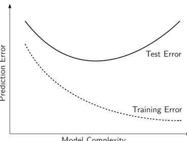
Err =ExtrEY0_,X0[L(Y0, ˆf(x0))| x_tr] =E_xtr[Err_xtr]. (2.2) An idealized illustration of the test and training error with respect to increasing model complexity is given in Figure 2.1. To assess the quality of a prediction rule the expected test error is the decisive quantity since it reflects best the performance of the prediction rule on future observations. In the following, we continue referring to the test error simply asprediction error. In practice it is often not possible to split the observations given into different data sets since there are too few observations. Then the prediction error can be estimated by cross-validation as we will discuss in Section5.3.3.

    Pr ed ic tio n Er ro r Model Complexity Test Error Training Error

Figure 2.1: Illustration of a model test and training error depending on the model complexity.

According to Hastie et al. (2009), under the weak assumption that

Y = f(x) +e

wheree, with E(e) =0 and Var(e) = σ2, represents the error term, residuum,

or noise, the expected prediction error of a prediction rule ˆf(x)at an input pointX= x0can be decomposed into

Err(x0) = E[(Y− fˆ(x0))2 | X= x0]

= σ2+ [E ˆf(x0)− f(x0)]2+E[fˆ(x0)−E ˆf(x0)]2

= σ2+ Bias2(fˆ(x0)) + Var(fˆ(x0)).

σ2is called the irreducible error since it is the variance around the true mean

f(x0)and thus independent of the prediction rule. To minimize the expected prediction error bias and variance of ˆf(x0)need to be traded-off:

• Bias2(fˆ(x0)) = [E ˆf(x0)− f(x0)]2:

The bias can be reduced including more variables.

• Var(fˆ(x0)) = E[fˆ(x0)−E ˆf(x0)]2:

The variance is increased if more variables are added, since more parameters need to be estimated and each estimation contributes more variance to the overall variance.

As mentioned before the main aim of prediction is to select a set of variables that minimize the expected prediction error. The variables selected

are not necessary optimal for interpretation. First, the “minimal-optimal” set does not include all variables related to the outcome. When two variables are highly correlated and have equal effects on the outcome, a good prediction rule needs to include only one of them and discard the other, because the second one does not add any new information. Furthermore, due to spurious correlation, a variable might be useful for prediction, though it is not related to the outcome. Ranking procedures that provide an “all-relevant” subset of variables are more suitable for interpretation.

Accurate prediction rules are especially important in the classification of cancer subtypes based on gene expression signatures. In clinical practice, some subtypes of cancer are difficult to discriminate in standard histology. Still, exact classification is vital to design and to employ the best fitting therapy. For example, Khan et al. (2001) discuss classification of the small, round blue cell tumors of childhood which can be divided in four subtypes, including neuroblastoma, rhabdomyosarcoma, non-Hodgkin lymphoma, and the Ewing family of tumors. The four subtypes are hard to distinguish in light microscopy. Other techniques for diagnosis, like immunohistochem-istry for the analysis of proteins or molecular markers based on PCR, fail to provide secure classification due to technical difficulties or too variable measurements (Khan et al., 2001). Using an artificial neural network, the authors are able to construct a classification rule based on gene-expression data of 63 training samples that correctly classifies 25 test samples. In Sec-tion6.3we illustrate in more detail that there exist clear genetic signatures that allow to discriminate between the subtypes with high precision.

Prediction can also be used to identify subtypes of cancer that exhibit distinct expression signatures. Diffuse large B-cell lymphoma are character-ized by heterogeneous clinical outcomes. Less than every second patient responds well to the given therapy and exhibits durable remission. More than half of the patients die of the lymphoma. Alizadeh et al. (2000) illus-trate different gene expression patterns depending on the malignancy of the tumor. Additionally, the authors suggest the definition of prognostic groups on the gene expression patterns and important clinical indicators. Depending on the prognostic group the course of therapeutic actions should be adapted. While standard treatment starts with chemotherapy and in case of failed complete remission takes up bone marrow transplantation, a specific prognostic group of patients should receive early bone marrow transplantation.

To sum up, prediction rules constructed on omics data may provide a valuable tool in clinical diagnostics if they can generalize to new data and predict accurately future cases. The central quantity to assess the perfor-mance of a prediction rule is the prediction error estimated on an indepen-dent test data set or by cross-validation. Variable selection in prediction aims at finding variables with good predictive effects that minimize the prediction error.

2.2.2

Ranking

In contrast, ranking procedures aim at selecting all relevant variables, the “all-relevant” set. These rankings are mainly used for interpretation and provide a “short-list” of interesting orimportantfeatures. Such a short list is especially relevant if the analysis is not hypothesis driven. This is the case when there is only scarce or no a priori information on the true effects and an abundance of possible variables is to be taken into account. Then, a ranking provides an explanatory tool for interpretation.

First, it is essential to define when a variable is important and how this notion of importance can be quantified by a score. For example, in the two group case, whereY is binary, predictor variables are important that discriminate well between the two groups. Thus, importance is often defined as the standardized mean difference which is quantified by the well-known t-score. An extensive discussion on the notion of importance can be found in Section3.2and Section4.3. Then, all variables are ordered according to decreasing importance. Finally, a cut-off is set to distinguish between variables of interest ornon-null or nonzero variables at the top of the list and uninteresting variables or nullor zero variables at the bottom of the list. It is recommended to fix the cut-off in a way to control the number of false positives included in the variables selected. If the number of variables is small standard hypothesis tests with significance levels adjusted for multiple testing can be used. For high-dimensional settings control of the false-discovery rate is wide-spread (Benjamini and Hochberg, 1995). More details on how to determine a cut-off are given in Section5.3. In practice, it is desirable to validate the top-listed variables. Constraints in financial resources or constraints of the techniques used in the follow-up experiments lead to ad-hoc determinations of the cut-offs. For example, qPCR is often used as cheap low-throughput technique for validation of high-throughput gene-expression experiments. Since qPCR captures the expression of only few genes, e.g. 20 genes, the top 20 genes of the ranking are considered for follow-up experiments.

To assess the performance of a ranking quantities are used that are based on:

• True positives (TP):

Non-null variables correctly identified as non-null variables.

• False positives (FP):

Null variables incorrectly labeled as non-null variables.

• True negatives (TN):

Null variables correctly identified as null variables.

• False negatives (FN):

The use of the true positive rate (Sensitivity: _TPTP_+FN) and the true negative rate (Specificity: _TNTN_+FP) is widespread. A combination of those is repre-sented in the receiver operating characteristic (ROC). In case of skewed classes, i.e. when there is only a small fraction of either non-null or null variables, the use of ROC-curves is discouraged in favor of precision (True discovery rate) and recall (True positive rate, sensitivity, power):

• Precision = _TPTP_+FP

• Recall= _TPTP_+FN

Ranking is especially popular in the analysis of transcriptomics, where gene-lists often present the genes highly associated with the outcome of interest. For example, Pomeroy et al. (2002) analyze the differences in gene expression depending on the outcome of central nervous system embryonal tumor. Since there is little knowledge on the molecular basis of the tumor, the analysis is conducted in an explanatory fashion to elucidate markers related to the outcome. Thus, the authors compile two lists of genes, one with genetic markers for survival and one with genetic markers for treatment failure. In a similar fashion Singh et al. (2002) investigate gene expression profiles of patients suffering from prostate cancer. The authors compile a list of 29 genes correlated to the Gleason score that quantifies the degree of tumor cell differentiation.

To conclude, ranking procedures are valuable tools in explanatory studies that facilitate interpretation. Variable selection in ranking aims at finding all variables related to the variable of interest, the true positive effects, while controlling the number of false positives contained in the list.

Variable selection in classification

Classification is the general term for methods that model a categorical out-come Ythat represents the membership to one of K classes or groups. It is important that the number of possible classes K is limited, classes are disjoint, and the membership to a class is unambiguous. For illustration, this thesis focuses on the two-group case where K = 2. i.e. Y is a factor variable with only two possible realizations:

Y=

(

1 if the observation belongs to group 1 2 if the observation belongs to group 2

A generalization to K > 2 is straightforward (Ahdesmäki and Strimmer, 2010), thus this thesis gives only a short sketch of multi-class classification. First, strategies for prediction are discussed. These include discriminant analysis and logistic regression. Then, quantities for variable ranking are presented. Here, variants of thet-score are widespread. After presenting established methods we introduce a novel approach to variable selection under correlation, correlation-adjustedt(CAT) scores. We show that CAT scores are the natural approach to ranking variables under correlation since they are motivated from linear discriminant analysis which is the classical approach to prediction in case of correlated predictors. Furthermore, we discuss the most important properties of the CAT score, point at relations to other quantities, and present strategies to estimate them in high-dimensional data. Finally, the performance of prediction and ranking strategies is exam-ined in simulations. For application of CAT scores on real omics data we refer to Section6.3and Section6.4.

3.1

Prediction

For prediction this thesis focuses on linear models for classification, (linear) discriminant analysis and logistic regression. Linear refers to the decision

boundary that is modeled to discriminate between the groups. There exist various techniques that provide more flexible solutions, like nearest neighbor classifiers, support vector machines, or neural networks. For an extensive overview see Hastie et al. (2009). Although linear models might seem to be of dusted quality compared to modern computer-intensive techniques, they are highly popular in practice. The popularity of linear models is due to the well-established statistical framework, interpretable results, and efficient performance (Hand, 2006).

3.1.1

Discriminant analysis

Discriminant analysis is based on the assumption that the d predictor or explaining variablesX follow the gaussian distribution with differing pa-rameters depending on the class-membershipY =k. Each classk ∈1, ...,K

is represented by a multivariate normal distribution

f(x|k) = (2π)−d/2|Σk|−1/2 × exp{−1 2(x−µk) T_Σ−1 k (x−µk)} with

• the vector of expectationsµ_kof lengthd, and

• the covariance matrixΣk of sized×dthat has the variancesσ_i2, with

i ∈1, ...,d, on its diagonal.

The multivariate normal distribution is solely determined by these two pa-rameters. There are three different types of discriminant analysis depending on the restrictions on the covariance matrixΣk:

• Diagonal discriminant analysis (DDA):Σk =diag(σ₁2, ...,σ_d2)

assumes no correlation among the predictor variables X, but differ-ing variances σ2. In machine learning DDA is often referred to as

‘independence rule’ or ‘naive Bayes’ (Bickel and Levina, 2004).

• Linear discriminant analysis (LDA):Σk =Σ

relaxes the assumption of DDA to the presence of correlation among the predictor variablesX. But there isno difference in covariance structure between the groups. That is allKgroups have the same covarianceΣ.

• Quadratic discriminant analysis:

further eases the restriction of equal covariances and allows different covariancesΣkin all Kgroups. Nonetheless, quadratic discriminant analysis is seldom used in practice since K covariance matrices of sized×dneed to be estimated. The remainder of this thesis neglects

quadratic discriminant analysis since it is impracticable in the analysis of high-dimensional data.

For classification the probability of belonging to classkconditional on the predictorsX is decisive. In discriminant analysis this conditional proba-bility for classkgiven the data is derived using Bayes’ theorem. The joint distribution ofX is given by a mixture of allKconditional distributions with a priori mixing weightsπk

f(x) =

K

∑

k=1

πkf(x|k).

Using the conditional distribution f(x|k)and the joint mixture density f(x)

Bayes’ theorem gives the posteriori probability of groupkgiven the data,

Pr(k|x) = πkf(x|k)

f(x) .

In turn the conditional probability defines the discriminant scoredk(x) =

log{Pr(k|x)}. Thediscriminant scoreis the pivotal element of discriminant analysis as it is the basis for classification. In LDA it is possible to drop terms constant across groups to simplify the discriminant scoredLDA_k (x)to

dLDA_k (x) = µT_kΣ−1x−1 2µ T kΣ −1 µ_k+log(πk). (3.1)

Due to the common covariancedLDA_k (x)is linear inx, hence the name of the procedure. For DDA the discriminant score reduces to

dDDA_k (x) = µT_kV−1x−1 2µ T kV −1 µ_k+log(πk) (3.2)

where V = diag(σ₁2, ...,σ_d2)is a d×d matrix with the variances ofX on its

diagonal.

In the two group case (K =2) the prediction rule is given by the differ-ence between the two discriminant scores

∆(x) = d1(x)−d2(x) = log{Pr(k =1|x)} −log{Pr(k=2|x)}. (3.3) The assignment to class 1 or 2 depends on the sign of the prediction rule; if

∆(x) ≥0 the observation is classified to group 1, for∆(x) <0 it is classified to group 2. In classification of more than two classes an observation is assigned to the classkwith the highest a posteriori probability Pr(k|x) or discriminant scoredk(x).

A different representation for multi-class classification is given by the pooled centroid formulation. Here, the pooled mean over allK classes is

given by µ_pool = K

∑

Following Equation3.1the pooled discriminant score is given as

dLDA_pool(x) = µT_poolΣ−1x−1

2µ

T poolΣ

−1

µ_pool.

Then, the centered prediction score for classkis

∆k(x) = dk(x)−dpool(x).

For prediction, this centered prediction score is equivalent todLDA_k (x)and analogously an observation is assigned to the classkwith the highest cen-tered prediction score.

In practice, the mixing probabilities πk, the expectations µk, and the

covarianceΣneed to be estimated and plugged into the discriminant score.

• The mixing weightsπk represent the a priori probability of belonging

to groupk. It is estimated by the relative frequency of groupkin the sample. In the two group case 1=π1+π2holds.

• If there are more observations than variables (n > d) empirical esti-mates can be used, like the arithmetic mean for the expectation and the covariance estimate

ˆ µ(x) = x¯ = 1 n n

∑

∑

• In settings with small n, large d, the estimation of the covariance matrix is intricate since the dimension of the d×d matrix becomes prohibitively large. There are two strategies, the first is to apply regu-larized estimates on the covariance matrix, like shrinkage estimates (Schäfer and Strimmer, 2005) orL1 penalties (Witten and Tibshirani, 2011). Otherwise it is possible to discard the correlation among the predictor variables which is equal to a diagonal covariance matrix, i.e. restrict to DDA (Bickel and Levina, 2004).

• The widely-used prediction analysis for microarrays (PAM) algorithm (Tibshirani et al., 2002) is based on the independence assumption from DDA. Moreover, it applies shrunken centroids to perform an inherent selection of variables by a soft threshold. The standard centroid defini-tionckwith regularization for the standard deviation for classkwith

expectationµ_kis given as the standardized difference

ck =

µ_k−µ_pool

σ+s0

wheres0is a positive constant to stabilize the estimation of the variance since too small values in the denominator can lead to large values in ck. This is equivalent to

µ_k =µ_pool+ (σ+s0)ck.

PAM replaces the centroidsck by shrunken centroidscλ_k that are

de-fined by a soft threshold with a constantλ

cλ

k =sign(ck)(| ck | −λ)+

where + denotes the positive part and zero otherwise. The penalization parameterλis determined by cross-validation. Using these shrunken

centroids PAM applies the following expectations for classk

µλ_k =µ_pool+ (σ+s0)cλk .

Thus, any variableXiwith(| cik | −λ) <0 for allkdoes not contribute

to the prediction, sinceµλ_k =µ_pool. Finally, the discriminant score of

PAM is defined as

d_kPAM(x) = (x−µλ_k)TV−_PAM1 (x−µλ_k)−log(πk)

whereVPAMis a diagonal matrix with(σ+s0)2on its diagonal. PAM is implemented in theR-packagepamr.

3.1.2

Logistic regression

Generalized linear models allow to model responses that follow distribu-tions different from the gaussian distribution. IfY follows a distribution that can be expressed as an exponential family, it is possible to define a link functiongthat allows to model a linear relationship between the response

Y and the linear predictor η = β0+βTX (Fahrmeir and Tutz, 2001). In

particular, for classification in the two group case the logit link is the most popular one. Using the logit link the probability of membership to class 1 given the data yields the linear predictorη

g(Pr(k=1| x)) =log{ Pr(k =1| x)

In turn Pr(k=1| x)can be expressed by the inverse transformation

Pr(k =1| x) = g−1(η) = exp(η)

1+exp(η).

Using the notation of the regression coefficients the probabilities of belong-ing to class 1, respectively class 2, dependbelong-ing onX are given as

Pr(k =1|x) = exp(β0+β T x) 1+exp(β0+βTx) , Pr(k =2|x) = 1 1+exp(β0+βTx) .

Like in the linear discriminant analysis, thedpredictor variablesX follow a mixture of two normal distributions with different expectationsµ1andµ2 but common covariance matrixΣ. The a priori mixing weights are given asπ1andπ2 =1−π1, respectively. Then, the intercept β0and regression coefficients βcan be expressed as (Efron, 1975)

β0 =logπ1 π2 −1 2 µT₁Σ−1µ₁−µT₂Σ−1µ₂ , βT = (µ₁−µ₂)TΣ−1. (3.5)

There is a close connection between LDA in the two group case and logistic regression: The discriminant function in LDA in Equation3.3corresponds to the logit link model in Equation3.4

∆(x) (=3.3)d1(x)−d2(x) =log{Pr(k=1|x)} −log{Pr(k =2|x)}=

=log{ Pr(k =1| x)

1−Pr(k =1| x)}

( 3.4)

= g(Pr(k =1| x)).

Still, the estimation of coefficients differs in the approach and its efficiency (Efron, 1975). In contrast to LDA, where only estimates of covariance and expectation are plugged in to derive estimates for the discriminant function, in logistic regression the estimatesb0andbof the regression coefficients are obtained by maximizing the conditional likelihood with respect tob0andb

fb0,b(y1, ...,yn | x1, ...,xn) = n

∏

Maximum likelihood estimation is only possible if there are more obser-vations than variables. Otherwise regularized approaches are needed. A detailed overview of regularized regression is presented in Section4.2.

3.2

Variable ranking

The ranking of variables in classification is based on measures of variable importance. A variable is considered as important ifit helps to discriminate between the K classes. As in the previous chapter the focus is on the two-group case. First, the t-score is introduced as a standard criterion for variable importance to compare two groups. Furthermore, the relation of t-score and diagonal discriminant analysis is discussed. Since thet-score suffers from unstable estimates in the analysis of high-dimensional microarray data regularization strategies are presented in the following section, including the well-established strategies SAM (Tusher et al., 2001), shrinkaget (Opgen-Rhein and Strimmer, 2007c), and moderatedt(Smyth, 2004).

3.2.1

Quantities for variable importance

In classification a (explanatory) variableXi inX is considered as important if it discriminates between the groups defined by the variable of interestY. The dominant quantity of importance in the two-group case is thet-score. The empiricalt-score for variablexi is defined as the difference between the

mean ¯x1(i)in group 1 and the mean ¯x2(i)in group 2, standardized with the sample sizen1in group 1, respectively the sample size n2in group 2, and the sample variances2(i)

t(i) = ( 1 n1 + 1 n2 )s2(i) −1/2 (x¯1(i)−x¯2(i)). (3.6) Depending on the assumptions on the variance different estimates are ap-plied. For equal variances in the groups the following estimate is used

s2(i) = (n1−1)s 2 1(i) + (n2−1)s22(i) n1+n2−2 with s2₁(i) = 1 n1−1 n1

∑

∑

t-test checks if there is a difference in means of one metric variableX in two groups defined by a binary factorY. The (two-sided) null hypothesis is given as µ1 = µ2, i.e. there is no difference in means between the two groups. Under the null hypothesis thet-score follows thet-distribution with

A special case of the t-score is the assumption that all variances are equal, that is σ₁2 = ... = σ_d2. Then, the t-score is proportional to the fold

change defined as the mean differences between the two groups. A different definition for the fold change is the ratio of the two mean differences; in this thesis, the definition of mean differences is used. Since microarray data is often log-transformed in the preprocessing step it holds that log(µ1

µ₂) =

logµ₁−logµ₂.

Interestingly, there is a close connection between thet-score and diag-onal discriminant analysis. Let τ be a multivariate representation of the

d-dimensionalt-score vector, where the estimated variance S =diag(s2(1), ...,s2(d))is replaced by the population variance V =diag(σ₁2, ...,σ_d2),(_n1

1 + 1

n2)by a constantcn and the means by the expec-tationsµ₁, respectivelyµ₂

τ ={cnV}−1/2(µ₁−µ₂). (3.7)

The constantcn is a scale factor inherent in thet-score that depends only on the sample size in the two groups and is constant for alldvariables. Thus, it is negligible in ranking thedvariables. In the following, this thesis discrimi-nates betweenτ, thet-score on thepopulation level, andt, the definition of

theempirical t-score.

Recalling the prediction rule in DDA as difference in discriminant scores (Equation3.2) we decompose the prediction rule into a weight vectorωDDA,

independent ofX, and a vector-valued distance functionδ(x)

∆DDA_{(x) = d}DDA 1 (x)−dDDA2 (x) = µT₁V−1x−1 2µ T 1V −1 µ₁+log(π1) − µT₂V−1x−1 2µ T 2V −1 µ₂+log(π2) = (µT₁ −µ₂T)V−1x−1 2 (µT₁ −µ₂T)V−1(µ₁+µ₂) +log(π1 π2 ) = (µT₁ −µ₂T) | {z } 1×d V−1 |{z} d×d x−1 2(µ1+µ2) | {z } d×1 +log(π1 π2 ) = (µT₁ −µ₂T)V−1/2 | {z } ωDDAT · V−1/2 x−1 2(µ1+µ2) | {z } δ(x)DDA +log(π1 π2 ) = ωDDAT | {z } 1×d δ(x)DDA | {z } d×1 +log(π1 π2 ). (3.8)

This decomposition illustrates the main constituents of the DDA prediction rule:

• A constant governed by the a priori mixing properties, log(π1 π2),

• the vector-valued distance function δ(x)DDA that quantifies the

dis-tance of the variables X to the overall mean µ1+µ2

2 corrected for the variances

δ(x)DDA =V−1/2(x− µ1+µ2

2 ),

• a weight vector, independent ofX

ωDDA =V−1/2(µ₁−µ₂).

Thus, the weight vector ωDDA controls the influence of a standardized

variableδ(x)on the prediction rule. Here, the weight vector ωDDA is

pro-portional up to the constant cn to the t-score vector τ as defined on the

population level in Equation3.7. In the following,ωDDA is interpreted as an

unscaled version of the populationt-scoreτ. Moreover, this decomposition

shows that thet-score is the natural quantity to measure the importance of a variable on the prediction rule in case of uncorrelated explanatory variables. Hence, thet-score is theoptimal criterionto select variables for prediction if there isno correlationamong predictors (Fan and Fan, 2008).

3.2.2

Regularized estimates

The previous section has introduced the standard definition of thet-score, that may suffer from a severe defect in practice due to the presence of small variances near zero. Then, the standard deviation tends even more to zero and the t-score from Equation3.6as ratio of mean difference to standard deviation tends to infinity even for small to moderate differences in mean. Thus, the standardt-score is prone to high values due to small variances that are usually considered as unimportant for biological interpretation. For interpretation the mean difference is much more important. To overcome this instability in estimation regularized versions of thet-score have been introduced. The first publication on a regularizedt-score is by Kerr et al. (2001). Since then several versions oft-scores have been introduced. Reg-ularizedt-scores modify Equation3.6by adding a small constants0to the denominator treg(i) = (x¯1(i)−x¯2(i)) √ cn(s(i) +s0) . (3.9)

All regularizedt-scores share the same generalized definition from Equa-tion 3.9 but they differ in how to derive the denominator, especially the

constants0. The following section gives a short introduction to three estab-lished regularizedt-scores: SAM (Tusher et al., 2001), moderatedt(Smyth, 2004) and shrinkaget(Opgen-Rhein and Strimmer, 2007c).

• SAM is the abbreviation for significance analysis of microarrays and is implemented in theR-packagesamr. Here, the constants0in Equa-tion3.9is set to minimize the coefficient of variation.

• The moderatedtis derived from a hierarchical model, where prior in-formation on the variances(i)is modeled by an inverseχ2-distribution

with d0degrees of freedom 1

s2_(i) ∼ 1

d0s2₀

χ2(d0).

This prior is incorporated into the posterior variances2(i)mod that is

represented by a mixture of the sample variance s(i) and the prior variances0 s2(i)_mod = dg dg+d0 s2(i) + d0 dg+d0 s2₀.

The amount of mixture is governed by the a priori degrees of free-domd0and the sample degrees of freedomdg. Finally, this posteriori variance is plugged into the denominator of Equation3.9. Thus, the moderated t is proportional to an ordinary t-score by the constant

cn but instead of using the sample variance a mixture of sample and prior variance is used to stabilize thet-score. The prior parameters

d0ands0are estimated from the data in an empirical Bayes approach. Moderatedtis implemented in theR-packagelimma.

• In contrast to the moderatedtthe shrinkagetmakes no assumptions on the distribution of the variance. The shrinkagetis derived from the James-Stein rule. A generalized illustration of a James-Stein ensemble estimateθshrinkfor an unknown parameter vectorθof lengthdis based

only on three components

θshrink = (1−λ)θˆ+λθtarget (3.10)

with

– θˆ as an unregularized estimate forθ,

– θtarget as the target estimate, and

– λas the parameter to govern the amount of shrinkage.

The target estimateθtarget is specified using a priori information. E.g.