Outlier Identification in Spatio-Temporal Processes

(1)

Outlier Identification

in

Spatio-Temporal Processes

by

Shrijita Bhattacharya

A dissertation submitted in partial fulfillment of the requirements for the degree of

Doctor of Philosophy (Statistics)

in The University of Michigan 2018

Doctoral Committee:

Professor Stilian Stoev, Co-Chair Professor George Michailidis, Co-Chair Professor Veronica Berrocal

Research Scientist Michael Kallitsis Assistant Professor Gongjun Xu

(2)

Shrijita Bhattacharya [email protected]

ORCID iD: 0000-0001-6958-8613

c

(3)

(4)

ACKNOWLEDGEMENTS

I would like to express my heartfelt thanks to my adviser Professor Stilian Stoev for his constant guidance, valuable expert suggestions and encouragement. I would like to thank him for giving me the opportunity to work with him at the Department of Statistics, University of Michigan, and providing my research with financial support. I would also like to thank Professor George Michailidis and Dr. Michalis Kallitsis for their guidance and financial support on two of my projects closely related to the domain of engineering. I would like to thank Merit Network Inc for providing me with data on Internet traffic flows and Electricity consumption on power grids, an indispensable part of the work on anomaly detection in networks.

I would also like to thank all my friends in Ann Arbor and East Lansing, Michigan, especially Raka Mandal, Pramita Bagchi, Sebanti Sengupta, Anwesha Bhattacharya, Diptavo Dutta and Aritra Guha. Without their support and camaraderie, Phd life would have been a lot more difficult to cope up with.

Last, but not the least, I would also like to express my intense gratitude to my parents, Rita and Mrityunjoy Bhattacharya and my husband, Abir Chatterjee for their constant encouragement and motivation all along my Phd Career.

(5)

LIST OF FIGURES

Figure

2.1 Left: Power prediction (with 95-percentile bounds). Right: Model validation (real-data) . . . 7 2.2 Left: Detection alerts (red) over a two-day period. The vertical red

stripe denotes an hour-long period of injected anomalies. We study the behavior of each building; the building under study is consider as unobserved (unsecure) and we use observations from the remaining ones. An EWMA control chart was used with w = 1, L = 3.719. Right: The effect of clustering in detection performance. (Due to sorting, the building orderings in the top and bottom panels differ.) 14 2.3 High-level architecture of AMON. . . 19 2.4 Sketch data blocks are used as the basic input structures for our

detec-tion algorithms. The databrick matrix; notice the horizontal stripes that signify traffic from multiple destinations to multiple sources. Note also the bold column at source bin 100 that depicts heavy source(s) activity. . . 22 2.5 Left: View of source array, constructed by aggregating over the columns

of the matrix. Note the heavy source(s) at bin 100.Right: Destina-tions array; observe how heavy destinaDestina-tions appears as heavy bins. In all cases volume is in bytes in log scale. . . 23 2.6 Time-series of Source hash-binned arrays (Top) and its zoomed-in

version. (Bottom right), computed over 10-second windows. The max-spectrum of the entire time series is plotted on the bottom-left. Merit Network: 17:30-18:30 EST, July 22, 2015. . . 24

(9)

2.7 Merit Network 16:00-17:00 EST, Aug 1, 2015 – the ‘Tor’ event in Section refsubsec:tor. (Top left) Ingress connectivity for the top

N = 3000 hash-binned flows per 10-second windows over 1-hour. (Top-right) QQ-plots demonstrating accuracy of the Normal approx-imation of typical in-degree distributions. (Bottom plots) QQ-plots for anomalous bins. . . 32 2.8 Case Study of ‘Library’ event. Evaluation of our detection algorithm. 37 2.9 ‘Tor’ case study: Nature of the attacks. . . 38 2.10 ‘Tor’ case study: Attacks detected by community detection. . . 38 2.11 Visualizations readily available by our data products. Top:

Adja-cency matrices of co-connectivity graphs (node indices sorted by de-gree - black corresponds to locations of 1’s). Bottom: Size of max cliques over time during the ‘Tor’ case study (Section 2.2.7.2). By observing clique size changes in Dashboards like this, coupled with the detection method of Section 2.2.5, such seemingly innocuous low-volume events are captured. . . 40 3.1 Trimmed Hill Plot for 5 outliers and sample size 100. The first

knee occurs around k0 = 5. Left: Pareto(1,1) with k = 99. Right: Burr(1,0.5,1) with k = 30 (see (3.30)). . . 53 3.2 Performance for varying values of tail exponent ξ. Left and right

panels correspond to n= 100 and n= 500, respectively. . . 63 3.3 Performance for varying amount of outliers. Left and right panels

correspond to the number k0 and the proportion k0/k of outliers respectively. . . 64 3.4 Performance of robust estimators for 0.9P(α,1) + 0.1P(α,1000) at

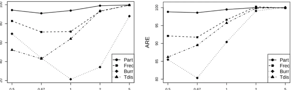
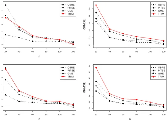
ARE=78%. Top left and right correspond to RB and RRMSE values for α = 1. Bottom left and right correspond to RB and RRMSE values for α= 3. . . 71 3.5 Performance of robust estimators where 5% observations of P(α,1)

are inflated by 10 at ARE=78%. Top left and right correspond to RB and RRMSE values forα = 1. Bottom left and right correspond to RB and RRMSE values forα = 3. . . 72

(10)

3.6 Performance of robust estimators for 0.9P(α,1) + 0.1P(α,1000) at ARE=94%. Top left and right correspond to RB and RRMSE values for α = 1. Bottom left and right correspond to RB and RRMSE values for α= 3. . . 73 3.7 Performance of robust estimators for 0.95P(α,1) + 0.05P(α,1000) at

ARE= 94%. Top left and right correspond to RB and RRMSE values for α = 1. Bottom left and right correspond to RB and RRMSE values for α= 3. . . 74 3.8 Performance of robust estimators at ARE=78%. Top left and right

correspond to RB and RRMSE values. . . 76 3.9 Performance of robust estimators at ARE=94%. Top left and right

correspond to RB and RRMSE values. . . 77 4.1 Spline basis functions evaluated. Left panel corresponds to the

peri-odic splines for seasonal activity, middle panel corresponds to splines for global activity and right panel corresponds to splines for ENSO activity . . . 86 4.2 Seasonal and trend components for historical temperature mean (top

panel) and standard error (bottom panel) curves over the period 1911-2010 for Ann Arbor, MI. . . 88 4.3 Standardized daily time series for Ann Arbor, MI. Left and right

pan-els indicate the standardized time series, Yt(s) and its corresponding

auto-covariance function. . . 89 4.4 Normal quantile-quantile plots for standardized weekly min Yt(s). Left

panel . . . 90 4.5 Distribution of the time seriesQk(u0) for varying values of the

quan-tile level u0 for the period 1911-2010. Extreme events in the series have been marked with red. . . 92 4.6 Thin spline interpolated time series Zk(s) for s ∈ D on time points

corresponding to extreme values of Qk(s) . . . 93

4.7 Histogram of the seasonal distribution of Qk > p for varying values of proportion p. . . 93 4.8 Extremal index for the time series Qk for varying declustering

(11)

4.9 Model Diagnostic Plot. . . 101 4.10 Scale parameter and shape parameters as a function ofk andx.. . . 103 4.11 Return level ˆrm for m= 10×365 as a function of Day and the ENSO.106

4.12 Return levels ˆrm form = 10×365 as a function of ENSO on various days of the year. . . 107 4.13 Return levels ˆrm for m= 10×365 as a function of year for different

levels of ENSO. . . 107 4.14 Return levels ˆrm for m= 10×365 as a function of year for different

levels of ENSO for u0 = 0.92,0.97 . . . 110 4.15 Quantiles for the distribution of Zk,∆(s) for varying values of ∆. The

gray lines represent different stations . . . 112 4.16 Return levels ˆrm for m = 10×365. Left panel: for ∆ = 2, ˆrm is a

function of day in year. Right panel: For ∆ = 14, ˆrm is a function of

the ENSO value. . . 114 4.17 Return levels ˆrm for m = 10 ×365 for ∆ = 7 at varying values of

the ENSO level. Left panel: ENSO=-1.5, Middle panel: ENSO=0, Right panel: ENSO=1.5. . . 115 4.18 Return levels ˆrm for m = 10×365 as function of window size ∆. . . 117

(12)

LIST OF TABLES

Table

2.1 Evaluation of detection performance (meter 1). . . 14

2.2 Silhouette values for cluster number selection. . . 15

2.3 Evaluation of detection Algorithm 2 in Section 2.2.3. . . 35

2.4 Evaluation of detection Algorithm 3 in Section 2.2.4. . . 36

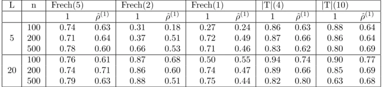
3.1 ARE of the adaptive trimmed Hill with respect to the classic Hill, k0 = 0 and ξ= 1. . . 60

3.2 ARE of the adaptive trimmed Hill k0 = 10, ξ = 1 and L > 1. For each distribution, top row corresponds to ARETRIM and bottom row indicates AREHILL. . . 61

3.3 ARE of the adaptive trimmed Hill k0 = 10, ξ = 1 and C > 1. For each distribution, top row corresponds to ARETRIM and bottom row indicates AREHILL. . . 61

3.4 ARE of the adaptive trimmed Hill relative to trimmed Hill for k0 = 10, ξ = andL <1. . . 65

3.5 ARE of the adaptive trimmed Hill relative to trimmed Hill for k0 = 10, ξ=1 andC < 1. . . 66

3.6 ARE of the adaptive trimmed Hill relative to trimmed Hill fork0 = 10. 69 3.7 Ratio of mean squared errors: adaptive trimmed Hill to trimmed Hill for k0 = 10. . . 70

4.1 AIC values for varying models M_i(σ)_,j(σ)_,i(ξ)_,j(ξ) with c (σ) 1 = c (σ) 2 = c(₁ξ)=c(₂ξ)= 3. . . 101

(13)

4.2 Estimates and their standard errors . . . 102

4.3 For u0 = 0.92, AIC values for varying models in (4.15) with c (σ) 1 = c₂(σ) =c₁(ξ) =c(₂ξ) = 3. . . 108

4.4 For u0 = 0.97, AIC values for varying models in (4.15) with c (σ) 1 = c₂(σ) =c₁(ξ) =c(₂ξ) = 3. . . 108

4.5 For ∆ = 2, AIC values for varying models in (4.15). . . 111

4.10 AIC values for varying models in (4.28) forc(₁σ) =c(₂σ) = 3 for different seasons. . . 119

(14)

LIST OF ALGORITHMS

Algorithm

1 Kriging for detection of data injection attacks. . . 12 2 Detection of heavy-hitter bins in traffic volume hash-arrays. . . 27 3 Flagging significant peaks in the relative volume of the top-k hash-bins. 30 4 Exponentially weighted sequential testing . . . 56 5 Joint estimation of k0 and k. . . 69

(15)

LIST OF APPENDICES

Appendix

A. AMON . . . 126 B. Robust Hill . . . 128 C. Spatial Extremes . . . 152

(16)

ABSTRACT

This dissertation answers some of the statistical challenges arising in spatio-temporal data from Internet traffic, electricity grids and climate models. It begins with methodological contributions to the problem of anomaly detection in communi-cation networks. Using electricity consumption patterns for University of Michigan campus, the well known spatial prediction method kriginghas been adapted for iden-tification of false data injections into the system. Events like Distributed Denial of Service (DDoS), Botnet/Malware attacks, Port Scanning etc. call for methods which can identify unusual activity in Internet traffic patterns. Storing information on the entire network though feasible cannot be done at the time scale at which data ar-rives. In this work, hashing techniques which can produce summary statistics for the network have been used. The hashed data so obtained indeed preserves the heavy tailed nature of traffic payloads, thereby providing a platform for the application of extreme value theory (EVT) to identify heavy hitters in volumetric attacks. These methods based on EVT require the estimation of the tail index of a heavy tailed dis-tribution. The traditional estimators (Hill (1975)) for the tail index tend to be biased in the presence of outliers. To circumvent this issue, a trimmed version of the classic Hill estimator has been proposed and studied from a theoretical perspective. For the Pareto domain of attraction, the optimality and asymptotic normality of the estima-tor has been established. Additionally, a data driven strategy to detect the number of extreme outliers in heavy tailed data has also been presented. The dissertation

(17)

concludes with the statistical formulation of m-year return levels of extreme climatic events (heat/cold waves). The Generalized Pareto distribution (GPD) serves as good fit for modeling peaks over threshold of a distribution. Allowing the parameters of the GPD to vary as a function of covariates such as time of the year, El-Ni˜no and location in the US, extremes of the areal impact of heat waves have been well modeled and inferred.

(18)

CHAPTER I

Introduction

Research on modeling, analysis and inference of spatio-temporal processes has been gaining pace over the last century owing to their predominance in many ap-plication domains such as Internet traffic, communication networks, climatic events, time evolving social networks, the stock market etc. In this dissertation, we analyze a pool of techniques for the detection of anomalous events in multivariate time series, each of which is contingent on the nature of data at hand. For example, electric-ity consumption patterns are naturally modeled by Gaussian distributions, whereas heavy tailed or power law distributions are prevalent in data arising from the stock markets or Internet traffic. Therefore this dissertation has developed a wide range of methods ranging from kriging, community detection to extreme value theory.

Chapter II. The first part discusses statistical tools for detecting intrusions and failures in the electric smart gridin order to prevent widespread power outages and/or breakdown of the electrical system in an area. A smart grid is composed of a multitude of components, each with its own functionality such as power generation, transmission and distribution. These components exchange information through the so called Advanced Meter Infrastructure (AMI), which facilitates efficient operation of the grid by allowing for near-real time adaptation to changes in demand. The AMI is often

(19)

vulnerable to attacks from malicious users especially from those with access to the state or topology of the electric grids. An example of this includes tampering of meter readings by introducing attack patterns which evade standard detection algorithms. An added disadvantage is the scarcity of resources or physical access needed for securing all the meters in the network. Kriging is a spatial prediction technique which allows for optimal estimation of unobserved quantities from available closely correlated observations. Therefore if a small subset of nodes in the network is secured, kriging may used to curb false data injections on the remaining untrusted nodes. If the size of the network is large, clustering based techniques may be used to obtain a subset of nodes with similar energy patterns and thus reduce the dimensionality of the problem. In Section 2.1.5, this method has been adapted for application to real-world building data from a large university campus.

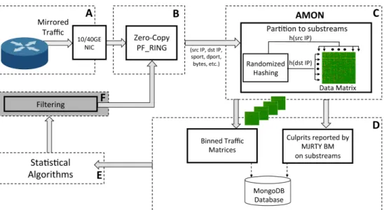
The second part of Chapter II involves a rather different spatio-temporal data arising from the monitoring of Internet traffic at a large regional Internet Service Provider (ISP). The predominance of Internet in every day life has made it all the more susceptible to attacks from a multitude of sources. Bank frauds, cyber threats, password hacks etc. have made the reliability of information transferred via Internet questionable. Many companies like Akamai are constantly updating their Content Delivery Network (CDN), to prevent Distributed denial of service (DDoS) attacks on their client networks. Network monitoring is essential to network engineering, capacity planning and prevention / mitigation of threats. Section 2.2 describes an open source architecture AMON (All-packet MONitor) deployed at Merit Network1 which is currently processing 10Gbps+ live Internet traffic. The main challenge in the analysis of network traffic is the shortage of memory resources for the storage of

(20)

information exchange for such a large network. Also most of the existing methods for anomaly detection are not scalable to the rate of flow for incoming traffic. To circumvent the issue of memory constraint, AMON partitions traffic into sub-streams by using rapid hashing and keeps track of heavy hitter2 IPs by employing a Boyer-Moore majority algorithm.

Application of optimally chosen hashing techniques preserve most of the important statistical properties of the underlying network traffic flows. These rapidly (online) computed hash-summaries may be thus used for identification of anomalous events in the network such as heavy hitters, DDoS, scanning or outrages. From statistical perspective, this can be cast into the problem of identifying outliers or change-points in multivariate, heavy-tailed time series. Volumetric attacks are identified as extreme outliers in the data and are best detected by the application of Extreme Value Theory. Specifically, robust and adaptive estimates of the heavy-tail exponent of the data are utilized to calibrate an anomaly detection threshold. On the other hand, the stealthier attacks arising from scanning or low-value DDoS are identified as high-connectivity events from a graphical data structure that quantifies the source-destination commu-nication patterns. This calls for other sophisticated techniques like the ones based on community-detection type statistics. These themes are addressed in Sections 2.2.3, 2.2.4 and 2.2.5.

Chapter III. Most of the detection algorithms of Section 2.2 in Chapter II require the estimation of the tail exponent of a heavy-tailed distribution. However, in the presence of outliers, the classic Hill estimator is biased and its variance also compromised. In Chapter III, we thereby introduce and study a trimmed version of the Hill estimator for the index of a heavy-tailed distribution, which is robust

(21)

to perturbations in the extreme order statistics. In the ideal Pareto setting, the estimator is shown to be finite-sample efficient among all unbiased estimators with a given strict upper break-down point. For general heavy-tailed models, the asymptotic normality of the estimator under second order regular variation conditions has been established. The estimator is shown to achieve the minimax optimal rate in the Hall class of distributions. A trimmed Hill plot to visually select the number of top order statistics has been proposed. The main contribution is the development of an automatic, data-driven procedure for the choice of trimming based on exponentially weighted sequential testing. This yields a new type of robust estimator that can adapt itself to the unknown level of contamination in the extremes. As a by-product we also obtain a methodology for identifying extreme outliers in heavy tailed data. The competitive performance of the trimmed Hill and adaptive trimmed Hill estimators is illustrated with simulations against several established robust estimators.

Chapter IV. Extremes of weather conditions, be it high or low, may have a devastating impact on the agricultural and industrial production of a country. As stated by Christopher R. Adams3:“In the US, the 1976 - 1977 winter freeze and drought is estimated to have cost $36.6 billion in 1980. In 1980 the nation saw a devastating heat wave and drought that claimed at least 1700 lives and had estimated economic costs $15 - $19 billion in dollars”. In Chapter IV, we develop a statistical framework for prediction of areal impact of heat waves. The methodology applies to cold waves as well. The approach adopted is the quantification of the area in US under profound heat wave activity at given time point. The Pickands-Balkema-de Haan theorem as well as extensive model diagnostic plots reveal that the generalized Pareto distribution, GPD serves as an efficient tool in modeling the peaks over threshold for

(22)

the so-obtained time series. Several other factors like intensity level of the heat wave, grid network of the US, season of the year and duration of heat wave events have been explored in connection to the analysis of heat wave distribution. As a main contribution, we obtain estimates for the out-of-sample return levels for a variety of heat wave events as a function of the season (time of the year), ENSO index and location in US. These estimates are based on the analysis of daily temperature records for a period of 100 years for 424 stations spread across the continental US.

In summary, the dissertation is organized as follows. Chapter II presents two different methodological contributions to anomaly detection in smart grids and com-puter networks, respectively. These methods motivate the study of robust estimators of heavy tail index in Chapter III. Chapter IV focuses on spatio-temporal infer-ence in the context of extreme heat wave events over the continental US. Finally the dissertation is concluded with the scope of each chapter.

(23)

CHAPTER II

Anomaly Detection In Networks

2.1 Security Of Smard Grid Electrical Units

Contributions and due credit: Much of the material in this section is a col-laborative work based onKallitsis et al.(2016c). As the author of the thesis, we have contributed primarily to the statistical aspects in Sections 2.1.2, 2.1.3 and 2.1.4 and the proof of Proposition II.1.

2.1.1 Introduction

Smart grid meters were developed to overcome some of the drawbacks of tradi-tional electric grids. For example, accurate estimation of the state of grid, incorpora-tion of renewable energy sources etc. are some of the features specific only to smart grids. The efficient communication between the various components of the smart grid is facilitated by advanced metering infrastructure (AMI). Engineers are mostly inter-ested in the security of AMI in order to ensure that the network can recover itself in the presence of anomalies/ power outages etcFarhangi (2010).

The susceptibility of the smart grids to attacks has increased only very recently. The smart grid infrastructure is often jeopardized by individuals who can manipulate

(24)

the meter readings or inject unwanted load into the system. Some such activities which have resulted in the breakdown of the grid include the Stuxnet worm and the attacks against Iranian nuclear facilities Falliere et al. (2011), the compromise of a steel mill in GermanyLee et al.(2014), and the cyber attacks on the Ukrainian power gird Lee et al. (2016).

In order to control for these malicious behavior, AMI meters are often accessed remotely. This however does not put an end to network changes caused by spoofed message payloads that carry power demand / supply values. Since the power con-sumption in an electric grid is usually determined by the state or topology matrix

H Liu et al. (2009), adversaries with access to it can severely compromise the meter readings. Over the past few years, a lot of research has been done on attack which can evade the security protocols of AMI (seeMcDaniel and McLaughlin(2009);Metke and Ekl (2010); Bed and DOE (2009); Yu (2015)).

0 1000 2000 3000 4000 5000 Time (2 minutes) 0 20 40 60 80 100 120 Po we r ( KW ) Ground Truth Prediction P values Frequency 0.0 0.2 0.4 0.6 0.8 1.0 0 50 100 150

Figure 2.1: Left: Power prediction (with 95-percentile bounds). Right: Model vali-dation (real-data)

.

In this section, a statistical methodology for the detection of bad data injection into wide-area smart grid networks has been proposed. We however make a crucial assumption that the attackers can access only a subset of the total number of avail-able meters. The other meters are however secure and can be used to predict the

(25)

energy consumption patterns of the remaining ones. Since in an electric network, a large number of meters are closely related in space (e.g., within the same residential neighborhood, university campus, town, etc.), the spatial algorithms which borrow strength from highly correlated observations may be used. Kriging is one such method and is suitable for the data at hand subject to some modifications.

For Section 2.1, we assume that trusted readings involve nodes that transmit encrypted data and whose identity is authenticatedBi and Zhang (2014). The set of these trusted nodes shall be referred to as the observed set and the remaining ones are categorized into the unobserved set. The rest of the work is organized as follows: Section 2.1.2 discusses clustering algorithms to group buildings with high correlation index in terms of electricity consumption, Section 2.1.3 details a factor model which illustrates the energy patterns in the network can be explained by just a few factor variables, Section 2.1.4 explains an adaptation of the kriging technique to allow for detection of anomalous observation in the system. Section 2.1.5 finally evaluates the proposed methodology when applied to real world electricity data from University of Michigan campus.

2.1.2 Building grouping

Let Y(t) = (Yi(t))i∈B be the time series of electricity usage for a set of B =

{1,· · · , B} buildings recorded over the time t= 1,2,· · ·,. For a monitoring window of size m, we define them×B as

(26)

Next the data Y(t)t=1,2,···, is partitioned into windows of size m and the mean

con-sumption for each window is considered as as

µ(t0, m) = 1 M M−1 X w=0 D(t0 −wm, m).

Treating each vectorµ(t0, m) as one observation, buildings with similar usage patterns can be identified by applying standard clustering techniques (K-means Kaufman and Rousseeuw (1990)) to µ(t0, m) for varying values of m.

2.1.3 Modeling power consumption via linear factors

Usingreal-world AMI building data (see Section 2.1.5), we observed that much of the variability in theY(t)’s can be explained by only few principal components of the matrix Q =PN

n=1Y(n)Y(n)

>_{. We therefore consider the eigen value decomposition}

of Q

Q=VΛV>

where V = [v1,· · · , vB] is a matrix with B orthonormal columns and Λ is a diagonal

matrix with entries λ1 ≥λ2 ≥. . .≥λB≥0 and propose the following factor model,

Y(t) = µY(t) +Z(t) := Fβ(t) +Z(t), (2.2)

whereFis a matrixB×k of factors,β(t)∈_Rk_{is a parameter estimable from data and} Z(t) is the measurement noise which follows multivariate normal distribution with zero mean and variance-covariance matrixΣ. The matrix Fconsidered is constructed from the firstkcolumns ofV which correspond to the eigen vectors forklargest eigen values. The factor model (2.2) serves as an adequate model for capturing the temporal variability of theY(t)’s (see Vaughan et al.(2013), Prop. 1). Since the factors Fand

(27)

Σremain constant only over shorter time scales, these are dynamically updated over moving time windows (see Algorithm 1).

2.1.4 Kriging-based prediction and detection

Using the factor model in (2.2), we next propose an anomaly detection methodol-ogy. Let Y(t) = (Yi1(t),· · ·, Yib(t)), {i1,· · · , ib} ⊂ B denote the electricity

consump-tion of buildings within the same cluster. We particonsump-tion meters into observed (trusted) nodes, O ⊂ {i1,· · · , ib}, and unobserved U = {i1,· · · , ib}\O. Let Yo = (Yj)j∈O and

Yu = (Yj)j∈U denote the partitioned vector Y (for notation simplicity we drop t).

Thus, from (2.2),    Yu Yo   ∼N    Fuβ Foβ   ,    Σuu Σuo Σou Σoo    ! . (2.3)

Given the limited set of observed nodes O, and if the true parameterβ is known, the minimum variance unbiased predictor ofYuis the kriging estimateCressie (1993a);

Vaughan et al. (2013):

ˆ

Yu(Yo, β) :=Fuβ+ΣuoΣ−oo1(Yo−Foβ). (2.4)

In practice, the parameter β is unknown, but can be estimated from data on the observed nodes using either a generalized least square regression :

ˆ

β= (F>_oΣ−_oo1Fo)−1F>oΣ

−1

(28)

or ordinary least squares as:

ˆ

β = (F>_oFo)−1F>oYo

For predictions for the unobserved nodesU, ˆβis used as the plug in estimator forβ

in (2.4). This also simplifies the expression for ˆYuto ˆYu =FuPYo+ΣuoΣ−oo1(I−FoP)Yo.

For detecting anomalies in the set of unobserved meters, we need the distribu-tion of the predicdistribu-tion errors (residuals) between the actual meter readings and their predictions, i.e., Ye =Yu−Yˆu.

Proposition II.1. Under the Null hypothesis of no anomalies and the model of (2.2), the prediction residualsYefollow a multivariate normal distributionYe ∼N(0,Σerr), with

Σerr=Σuu−CΣou−ΣuoC>+CΣooC> (2.6)

and C=FuP+ΣuoΣoo−1(I−FoP).

Proof. Observe that Ye = Yu −CYo is a linear transformation of Y, and therefore

Ye has a multivariate normal distribution. The expected error, µerr = E[Yu −CYo],

becomes µerr = FuE[ ˆβ]− CFoE[ ˆβ] from (2.2). PFo = I, which implies CFo =

FuPFo +ΣuoΣ−oo1(I−FoP)Fo = Fu, and, thus, µerr = 0. For the error variance,

Var(Yu−CYo) =_E(Yu−CYo)(Yu−CYo)>, and the result follows using (2.3). The prediction error Ye is used for identification of anomalies on the unobserved

meters. In this direction, we define the test statistic r2 ₌ _Y>

e Σ

−1

errYe, which

corre-sponds to the Mahalanobis distance whose p values can be obtained using Proposition (II.1) as

(29)

Algorithm 1Kriging for detection of data injection attacks.

Input: Training data D(t0) :={Yi(t), i∈ {1, . . . , b}, t0−N ≤t≤t0 };

Input: Set of “observed” nodes O;

Input: Set of “unobserved” nodes U ={1, . . . , b}\O;

Output: Sequence ofp-values for prediction errors.

1: Obtainb×k factor matrix Fusing PCA on data D(t0) 2: Estimate covariance matrixΣ using data D(t0)

3: for each new observation Y =Y(t), t=t0+ 1, . . . do 4: Partition vector Y into Yo and Yu

5: Estimation of ˆβ = (F>_oΣ−1

ooFo)−1F>oΣ

−1

ooYo =PYo.

6: Prediction: Yˆu =Fuβˆ+ΣuoΣoo−1(Yo−Foβˆ)

7: Calculate the error covariance matrix Σerr (see Eq. (2.6)) 8: With prediction error Ye:=Yu−Yˆu, get test statistic

r2 =Y_e>Σ−_err1Ye (Mahalanobis distance)

9: output p=1-F(r2_),_F₍_x_{) is a chi-squared cdf (d.f.=} _{|U |).} 10: end for

where F(x) is the chi-squared cumulative distribution function with degrees of free-dom equal to rank(Σerr). Algorithm 1 explains this entire methodology. To tame the false alarm rate, we apply an exponential weighted moving average (EWMA) control chart to the standardized z-scores z = Φ−1₍₁₋_p_{) (see also} _{Lambert and Liu} _(2006a); Kallitsis et al.(2015)), where Φ(x) is the cumulative distribution for standard normal.

2.1.5 Performance evaluation

This section uses the electricity consumption data from University of Michigan campus for evaluation purposes. The data set comprises of 163 buildings with obser-vations recorded at the time scale of every 2 minutes. The data is available for almost one year with a wide range of buildings such as health services, parking lots, student housing, laboratories etc.

Fig. 2.1 gives a plot for p values are generated by Algorithm 1 for observations from (2.2). As expected, behavior under true model is uniform. Fig 2.1 plots the p values generated from Algorithm 1 but with observations from the data set described

(30)

above. The uniformity in the p-value consolidates the model assumptions on the real data.

We next describe the simulation setting used for the evaluation of the proposed methodology. In these experiments, the factors and variance covariance matrix are obtained from a two week training period using Algorithm 1. For each building, the next 48 hours (720×48 observations) are predicted using observations from the remaining buildings. Finally EWMA control charts as described in Section 2.1.4 are used for determining out of control values. A simulated attack is injected at a randomly chosen epoch (lasting 1 hour or 30 observations) in the 48 hours span for the building under study. The detection accuracy of Algorithm 1 is determined in terms of the precision and recall (see Kallitsis et al. (2015)). We also evaluate the prediction accuracy for the building under study by the root mean square (rMSE) defined as rMSE = v u u t 1 T T X t=1 (Yi(t)−Yˆi(t))2

. For building 1, Table 2.1 reports these values for different pairs (w, L) when averaged over 50 independent realizations. The shift σ denotes the magnitude of the attack injected. As the value ofσ grows, the precision and recall improve thereby indicating the successful detection of the false attacks. The false positive rate may be further reduced considering the two-in-a-row rule Lucas and Saccucci (1990) or additional values for the EWMA pairs (w, L).

To get a unified picture of what happens to all buildings, we first fix a time point to inject attacks. Next a building is chosen and an attack is injected stretching for an hour from that point. The remaining observations are used for predicting the building under study and detecting the occurrence of an attack. This experiment is

(31)

w L Shift (×σ) Precision Recall rMSE (KW) 1.00 3.719 1 0.07 0.08 12.6 1.00 3.719 2 0.43 0.72 13.5 1.00 3.719 3 0.53 0.99 15.0 0.53 3.714 1 0.05 0.21 12.6 0.53 3.714 2 0.18 0.94 13.6 0.53 3.714 3 0.19 1.00 15.1 0.84 3.719 1 0.07 0.11 12.6 0.84 3.719 2 0.37 0.84 13.6 0.84 3.719 3 0.42 1.00 15.0

Table 2.1: Evaluation of detection performance (meter 1).

0 200 400 600 800 1000 1200 1400 Time (2 minutes) 0 50 100 150 Bu ild . N um . (so rte d b y a vg . c on su mp tio n) 0 20 40 60 80 100 120 140 160 −1.0 −0.5 0.0 0.5 1.0

Avg P ec. (Clust) - Avg Prec. (All Builds)

0 20 40 60 80 100 120 140 160 Building Number −1.0 −0.5 0.0 0.5 1.0

Avg Rec. (Clust) - Avg Rec. (All Builds)

De te ct io n A cc ur ac y: C lu st er in g Ev al ua ti on

Figure 2.2: Left: Detection alerts (red) over a two-day period. The vertical red stripe denotes an hour-long period of injected anomalies. We study the behav-ior of each building; the building under study is consider as unobserved (unsecure) and we use observations from the remaining ones. An EWMA control chart was used with w= 1, L= 3.719. Right: The effect of clus-tering in detection performance. (Due to sorting, the building orderings in the top and bottom panels differ.)

repeated for all building and the results are reported in Fig. 2.2 left. In vast majority of cases our methods detect the injected attacks, and that the false positive rate is relatively low in all tests. With increase in the number of observed nodes, the prediction accuracy improves but not substantially (results not reported here).

(32)

Cluster number 2 3 4 5 6 7 8 9 Silhouette score .81 .59 .60 .56 .52 .47 .43 .45

Table 2.2: Silhouette values for cluster number selection.

right examines the detection accuracy with and without clustering. The number of K-means clusters was selected by looking at the silhouette Rousseeuw (1987) scores (see Table 2.2); two main classes were identified. For a large number of buildings, clustering provided better detection accuracy in terms of the precision and recall values.

2.1.6 Conclusions

We have proposed an adaptation of the kriging model wherein the observations from a few trusted nodes are used to predict the energy patterns of the remaining ones. This naturally provides a method for the detection of bad data injection into a smart grid by recording predicted values which go outside the control chart limits. We verified these results in context of data from a wide area network, University of Michigan campus. To handle the issue of dimension when the number of buildings is large, clustering methodology has also been proposed.

Anomaly detection in smart grids can be broadly classified into three main cat-egories signature-, specification- and anomaly-based methods Berthier et al. (2010); Cleveland (2008); Wang and Lu (2013). Each of these methods has its own set of challenges. For example whereas new attacks with signatures agnostic to signature-based intrusion detection system (e.g., Snort) evade detection, specification-based systems Carcano et al.(2010) are difficult to tune. Our method primarily falls under the third category of anomaly detection. Other works in this direction include Kallit-sis et al. (2015); et al. (2013); Bi and Zhang (2014); Yu (2015). The idea of using a

(33)

few trusted node stems from Bi and Zhang (2014) which proposes a graph theoretic method for securing an optimal set of meter measurements so that state estimation is not compromised.

The main advantage of our method over the works inLiu et al.(2009);et al.(2010, 2013); Bi and Zhang (2014); Yu (2015), is that a prior of the system’s topology DC power flow model Liu et al. (2009); et al. (2010) is not needed and the the power consumption patterns suffice as an input variables. As a part of the future work we wish to incorporate the temporal variations in the data via autoregressive (both univariate and multivariate) processes. In addition, we wish to model the prediction patterns where the set of unobserved and observed nodes is unknown. Predicting the mean consumption patterns by known factors like building type, location, time of the day etc. may be an interesting extension to this work.

Acknowledgements: This work is supported by NSF grant CNS-1422078.

2.2 Online Monitoring Of Internet Traffic: Challenges And

Solutions

Contributions and due credit: Much of the material in Sections 2.2.2, 2.2.3, 2.2.4, 2.2.5, 2.2.6, 2.2.7 is based on the collaborative work Kallitsis et al. (2016a), done under the leadership of Dr. Michalis Kallitsis. As a author of the thesis, we have contributed primarily to the statistical aspects in 2.2.3, 2.2.4, 2.2.5, which would not have been possible without the real-world Internet data provided by the AMON infrastructure Kallitsis et al. (2016a,b) developed by Dr. Kallitsis’ team at Merit Network1_.

1_{Merit Network, Inc. operates Michigan’s research and education network. It serves a population}

(34)

2.2.1 Introduction

Over the years, Internet infrastructure has become more accessible but at the same time more vulnerable to security threats. Cyber attacks like Distributed Denial of Service (DDoS), port scanning, outages which are becoming increasingly common; can overwhelm the network rendering it completely dysfunctional. Czyz et al.(2014) presents a recent example of a large DDoS attack which was the outcome of mis configured NTP (network time protocol) servers. Other examples include reflection and amplification attacks from K¨uhrer et al. (2014); Rossow (2014) where multiple small requests are sent to several mis-configured NTP servers (or other UDP-based services).

The predominance of Internet in all spheres (banks, universities, industries) calls for the development of sophisticated tools which can help protect the system against malicious users. Some methods such as Snort (see, snort.org), Bro (bro.org) and Suricata(suricata-ids.org) which do exist are easily beguiled by malware existing in varying forms by encryption (polymorphic).Thus the problem of anomaly detection in Internet traffic requires a basic understanding of the network features in terms of traffic flows, its composition, capacity, quality of service etc. In the past a lot of sta-tistical work has been done in the direction of analyzing data from Internet, streaming algorithms Gilbert et al. (2001);Muthukrishnan (2005), tomography Xi et al.(2006); Lawrence et al. (2006) and analysis of heavy tails and long range dependence Stoev et al. (2005, 2006); Stoev and Michailidis (2010).

A communication network like Internet involves information exchange across a vast number of IP addresses. Storing information on traffic flows for all nodes is often a challenging task if not impossible. Sketch based algorithms developed in Krishnamurthy et al.(2003);Gilbert et al.(2007);Stoev et al.(2007) provide a solution

(35)

to this by constructing small summary structures which capture all essential features of the network. However, the amount of time taken in producing these sketches is quite large when compared to the rate of flow of incoming traffic. Another alternative to handling the storage constraint is using information available only through the packet headers like source/destination addresses, application ports, payload size etc. Tools like Netflow, sFlow etc. have been developed to facilitate the compression of packet data by grouping them into flows. However, their compression mechanism does not scale to the order at which packets arrive.

Even if it is possible to bypass the storage issue, there are relatively few algorithms which can detect anomalous events from sketches or Netflows. Such algorithms, if available are mostly sequential in nature and not deployable at shorter time scales. Thus even with the best practices like (e.g., BCP38 recommendation Senie (1998)), the identification and mitigation of events like Distributed Denial of Service (DDoS) still seems a distant goal. In this chapter, we thereby develop the statistical framework for AMON; a software which can read packet data from Netflows, compute real time statistical summaries and flag alarms on the onset of any unusual activity in the network (see Figure 2.3). In AMON, data is collected efficiently using a PF RING ZC module employed at Merit Network (see Section II C inKallitsis et al. (2016b)). The packet data so obtained is then summarized using optimal hashing techniques implementable at the time scale of routing (see Section II A inKallitsis et al.(2016b)). Our main contribution to this work has been the development of statistical al-gorithms which when applied to the hashed outputs can detect the onset of both volumetric and low lying DDoS. Some of the statistical approaches for detection of heavy hitters or frequent items in a stream have been developed inKarp et al.(2003); Cormode and Muthukrishnan (2005b); Cormode et al. (2003); Estan and Varghese

(36)

Figure 2.3: High-level architecture of AMON.

(2002); Gilbert et al. (2006); Krishnamurthy et al. (2003); Schweller et al. (2006); Cormode and Muthukrishnan (2004, 2005a); Porat and Strauss (2012); Gilbert et al. (2012). However most of these algorithms provide efficient solutions to the problem data storage rather than modeling the distribution of statistical flows. In this chapter, we show that the summary structures obtained from hashing are indeed heavy tailed and share most of the statistical properties of raw traffic. Thereby techniques from extreme value theory may be used for detection of heavy hitters, i.e. IPs contributing to unusually large traffic in the network. Sometimes smaller magnitude attacks may be launched by a large number of IPs working together in which case a rather differ-ent approach needs to be adopted. One such approach relies on recording of sudden appearances communities and cliques, etc.(see Ranshous et al. (2015)) in the graph of network flows. With a slight modification, this approach has been extensively used in the paper for identification of low lying attacks.

Once the onset of an anomalous event is recorded, the true IPs associated with it are traced back by using a extended version of the Boyer Moore majority algorithm

(37)

(see Section II B in Kallitsis et al. (2016b)). The rest of the Section is organized as follows: Section 2.2.2 describes how the synopsis data structures are constructed from by application of hashing. It also serves as the link between groups C and D in the architecture of AMON (see Figure 2.3) where the raw data in form of packets is summarized to a form which can be used by the statistical algorithms for anomaly detection. Sections 2.2.3 and 2.2.4 describes two detection algorithms based on the heavy tailed nature of the Internet data; a property which is preserved even after the application of hashing. These algorithm intend at identifying high volumetric attacks. These methods successfully identified the case where a DDoS attack was targeted at a public library of University of Michigan traffic (see Section 2.2.7.1). Section 2.2.5 presents an algorithm for detection of high frequency low magnitude attacks. This method which involves the source destination interaction matrix successfully identified low volume attacks targeted to Michigan servers from an autonomous system in Asia-Pacific (see Section 2.2.7.2). Finally a comparative performance of the methods. The detection accuracy of these proposed methods has been studied under simulation setting of Section 2.2.8.

2.2.2 Hashed binned data matrix and its visualization.

This section describes the construction of source destination flow matrix from the packet header information of payload transfer across the network. Every packet captured at the monitoring station can be viewed as a tuple (wn, vn) where wn is

the key and vn is the payload. In the context of Internet traffic, the key wn can

either denote an individual source/destination address or a source destination pair. The payload vn can represent file sizes in bytes, packets or network ports. Using

(38)

function f

f : Ω→V

for every incoming data point where Ω usually denotes the space of IPv4 addresses (Ω∈ {0,1}32_{) or their cross product (Ω}_{∈ {0}_,_1}64_{for source destination pair). Storage} of the signalf even for a small interval of time is practically impossible owing to the high speed of incoming traffic and large dimension of Ω. Therefore hashing techniques which can the distribute the space of IP addresses to a smaller number of bins have been employed. Precisely, a hash function h is represented as

h: [N]→[m] (2.7)

where [N] is the cardinality of Ω and [m] is the cardinality of the space over which the keys are distributed. Extensive details on the choice of the hash function are covered under Kallitsis et al.(2014) and Cormode and Muthukrishnan (2005b).

When a packet arrives for the key (s, d), one computes i=h(d) andj =h(s) and updates the sketch matrix as

X[i, j] =X[i, j] +v (2.8)

This sketch matrix is stored at the time scale of every 10s. Direct products of this matrix are the source and destination hashed arrays defined as

Source : Xt(i) = m X j=1 Xt[j, i] (2.9) Destination : Xt(i) = m X j=1 Xt[i, j] (2.10)

(39)

Source bin Dest bin 20 40 60 80 100 120 20 40 60 80 100 120 0 5 10 15 20

Figure 2.4: Sketch data blocks are used as the basic input structures for our detec-tion algorithms. The databrick matrix; notice the horizontal stripes that signify traffic from multiple destinations to multiple sources. Note also the bold column at source bin 100 that depicts heavy source(s) activity. The hash binned arrays (Xt(i))i=1,···,m will serve as the input to the statistical

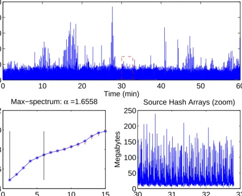
detec-tion algorithm of Secdetec-tions 2.2.3, 2.2.4 and 2.2.5. We next explore their distribudetec-tion properties for outgoing (Source) traffic at Merit Network for the period 17:30-18:30 EST on July 22, 2015. Figure 2.6 top panel shows a plot of the 360 hashed desti-nation arrays collected for a span of 60 minutes and then stacked one after another. The data reveals a few extreme peaks some of which may be attributed an attack event (see the ‘Library’ case study, Section 2.2.7.1). A zoomed in version on a short 3-minute period (bottom right panel) show that the extreme peaks, although of lower magnitude, persist. Apparent periodicities in extreme peaks may be attributed to data concatenation.

Data arising from Internet traffic such as file sizes, web page counts etc. are well modeled by heavy tailed or power law distributionsLeland et al.(1994);Crovella and Bestavros (1997); Faloutsos et al. (1999). This heavy tailed property is preserved even after the application of hashing (provided the hash function in (2.7) distributes

(40)

20 40 60 80 100 120 14 16 18 20 22 24 26 28 Sources bin

Bytes (log scale)

20 40 60 80 100 120 21.35 21.4 21.45 21.5 21.55 21.6 21.65 21.7 Destinations bin

Bytes (log scale)

Figure 2.5: Left: View of source array, constructed by aggregating over the columns of the matrix. Note the heavy source(s) at bin 100.Right: Destinations array; observe how heavy destinations appears as heavy bins. In all cases volume is in bytes in log scale.

the IP space uniformly). We thereby assume that X =Xt(i) satisfies

P(X > x)∼c/xα, asx→ ∞, (2.11)

where ∼ indicates asymptotic convergence and c, αare the parameters of power law distribution. Smaller values of α correspond to heavier tails. Indeed for α < 2, the mean does not exist and for α <1 both mean and variance are both undefined.

To validate the assumption in (2.11), we consider the max spectrum plot of an hour long time series of hash binned source traffic collected at Merit. The max spectrum is a plot of the mean log block maxima versus the log block sizes of the data. A linear trend indicates the presence of power-law tails with slope giving an estimate for 1/α. The linearity in the bottom panel of Figure 2.6 shows that power law is a fairly reasonable assumption for the time series of hash binned traffic. Steep slopes in the max spectrum plot correspond to heavier tails (low α). An advantage of the max spectrum plot is its ability to examine various log block sizes thereby allowing

(41)

0 10 20 30 40 50 60 0 200 400 600 800 1000

Source Hash Array Time Series (1 hour)

Time (min) Megabytes 30 31 32 33 0 50 100 150 200 250 Time (min) Megabytes

Source Hash Arrays (zoom)

0 5 10 15 24 26 28 30 32 Max−spectrum: α =1.6558 Log 2(block−size) Log 2 (block−maxima)

Figure 2.6: Time-series of Source hash-binned arrays (Top) and its zoomed-in version. (Bottom right), computed over 10-second windows. Themax-spectrumof the entire time series is plotted on the bottom-left. Merit Network: 17:30-18:30 EST, July 22, 2015.

for examination power law behavior in date varying time scales (see Stoev et al. (2011)). Extensive experimentation showed that the power-law behavior (linearity in the spectrum) extends over a wide range of time-scales from seconds to minutes with

α≈1.6 andα≈2.5 for shorter and intermediate time scales respectively (results not reported here). For larger time-scales (hours) complex intermittent non-stationarity and diurnal trends dominate and the heavy tailed characteristic of the data starts to breakdown.

Remark II.2. The hash-array is obtained from the PF RING-based methodology at the time scale of 10 seconds so that we do not run into the issue of empty bins and algorithms of Sections 2.2.3, 2.2.4 and 2.2.5 can be suitably applied. For higher traffic

(42)

rates, the methodology can be applied at an even shorter, sub-second time-scale.

2.2.3 Detection of heavy hitters

There has been a lot of work on the estimation of heavy hitters in fast network traffic streams Karp et al. (2003); Cormode and Muthukrishnan (2005b); Cormode et al. (2003); Estan and Varghese (2002); Gilbert et al. (2006); Krishnamurthy et al. (2003); Schweller et al. (2006); Cormode and Muthukrishnan (2004, 2005a); Porat and Strauss (2012); Gilbert et al. (2012). The definition of a heavy hitters is not explicit and is often open to interpretations. In this section, we introduce a rather new terminology in connection to the hash array inputs (2.9) where hash bins with abnormally large traffic are identified as heavy hitters. By abnormally large we mean observations which lie well above the quantile threshold for the baseline probability distribution of hashed inputs. Since the nature of traffic changes quite frequently, the baseline model needs to be dynamically updated while accounting for robustness and adaptivity issues (see last paragraph under Section 2.2.3). Lastly the type I error for the proposed test based algorithm is controlled by the choice of the quantile threshold. In Section 2.2.2, we showed the heavy tailed nature of the hash binned arrays defined in (2.9) (see Figure 2.7). For the source arrays, Xt(i) corresponds to the

number of bytes originating from all source IPs ω hashed to bin i, i.e. h(ω) =i over the time-window t. Optimal hashing techniques Kallitsis et al. (2014) and Cormode and Muthukrishnan (2005b) randomly distributes the IP addresses which more or less ensures that Xt(i), i= 1, . . . , m are independent and identically distributed (i.i.d.).

Abnormally large values of Xt(i)s, forsomei’s correspond anomalous events such

(43)

hash-array:

Dm(Xt) := max

i=1,...,mXt(i). (2.12)

Proposition II.3. Let X(i), i= 1, . . . , mbe i.i.d. random variables with heavy tails as in (2.11). Then, as m→ ∞, we have that

1 m1/αDm(X)≡ 1 m1/α_i₌₁max_,...,mX(i) d −→c1/αZα, (2.13)

where P(Zα ≤ x) = e−1/xα has the standard α-Fr´echet distribution and c is the asymptotic parameter in (2.11).

The proof is included in Section A.

A bin i∈ {1, . . . , m} is a heavy hitter, if its value is large, relative to the asymp-totic approximation of Proposition II.3. Section 2.2.6 shows that the asymptotic approximation kicks in even at values of m close to 128. We next define a heavy hitter formally as:

Xt(i)≥Tp0(m, α, c) :=m 1/α_c1/α_Φ−1 α (p0) = c log(1/p0)) 1/α , (2.14)

where the sensitivity levelp0controls the type I error rate and Φ−α1(p) = (log(1/p))

−1/α_, p ∈ (0,1) is the inverse of the standard α-Fr´echet cumulative distribution function Φα(x) = e−1/x

α

, x >0. By increasing p0 one can indeed reduce the number of false alarms (see Section 2.2.6). The methodology is summarized in the formal algorithm (Algorithm 2).

Several methods exist for the estimation of the parameters α and c (Embrechts et al. (1997),Hill (1975)). We however use the max-spectrum method in Stoev et al. (2011) since it is computationally efficient and easier to tune. In order to reduced the

(44)

Algorithm 2Detection of heavy-hitter bins in traffic volume hash-arrays.

Input: Stream of hash-arrays Xt ={Xt(i)}mi=1; probability level p0 ∈(0,1); smooth-ing coefficient λ∈(0,1).

Output: Stream of significant heavy-hitter bins Ht ⊂ {1, . . . , m} and their counts kt=|Ht|.

1: for each stream item Xt do

2: Estimate the tail exponent ˆα:=α(Xt) and scale coefficient ˆc:=c(Xt) from the

sample Xt={Xt(i)}mi=1 based on the max-spectrum. 3: if (t= 1) then

4: Set αt := ˆα and ct:= ˆc

5: else

6: Perform EWMA smoothing: αt :=λαˆ+ (1−λ)αt−1 and ct :=λˆc+ (1− λ)ct−1.

7: end if

8: Compute the significance threshold Tt:=Tp0(m, αt, ct) using (2.14).

9: Estimate the set of heavy hitter binsHtat windowtasHt:=

n i∈ {1, . . . , m} : Xt(i)≥Tt o . 10: return Ht and kt:=|Ht|. 11: end for

susceptibility of estimates to outliers, we apply an EWMA smoothing to the values of ˆα and ˆc (see Step 6 in Algorithm 2). The choice of the smoothing parameter is described in details under Section 2.2.6.

2.2.4 Relative volume

In the previous section we discussed heavy hitters from an absolute threshold standpoint (2.14). In this section, we analyze the scenarios where a small proportion IPs generate abnormally large traffic relative to the remaining ones. In this direction, consider the hash binned arrays in (2.9) and sort them in decreasing order as

(45)

Then for a fixed integer k ∈ {1, . . . , m}, we consider the relative volume of traffic contributed by the top-k bins:

Vt(k) := Pk j=1Xt(ij) Pm j=1Xt(ij) . (2.15)

These top-k bins may easily change from one time-window to another. High volu-metric attacks launched by a small subset of k IPs relative to the rest produce large values ofVt(k). In order to obtain significantly large values of Vt(k), we determine its

distribution using the heavy tailed property of the Xt(i)0s (see Section 2.2.2). This

baseline distribution is updated periodically similar to the previous section.

The following fundamental representation results for the joint distribution of the order statistics (see, e.g., p. 189 in Embrechts et al. (1997)).

Theorem II.4 (R´enyi representation). LetU(1), . . . , U(m)be independent and iden-tically distributed Uniform(0,1)random variables. Consider the sorted sample (order statistics) U(i1;m) ≤ · · · ≤U(ik;m)≤ · · · ≤U(im;m). Then, we have the following

stochastic representation: U(i1;m),· · · , U(ik;m),· · · , U(im;m) _d = Γ1 Γm+1 ,· · · , Γk Γm+1 ,· · · , Γm Γm+1 ,

where =d means equality in distribution and Γi =E1 +· · ·+Ei, i= 1, . . . , m+ 1 are Gamma(i,1)-distributed random variables, represented as cumulative sums of a fixed set of independent standard Exponential random variables.

In the previous section we argued that Xt(i), i = 1, . . . , m be i.i.d. with dis-tribution as in (2.11). For a continuous disdis-tribution function (cdf) F is U(i) :=

(46)

complementary cdf. Therefore, by Theorem II.4, F(X(i1)),· · · , F(X(ik)),· · · , F(X(im)) _d = Γ1 Γm+1 ,· · ·, Γk Γm+1 ,· · · , Γm Γm+1 .

By applying the inverse function F−1 to all components of the above relation, we obtain X(i1),· · · , X(ik),· · · , X(im) _d =F−1 Γ1 Γm+1 ,· · ·, F−1 Γk Γm+1 ,· · · , F−1 Γm Γm+1 . (2.16) This yields the following result about the distribution of the relative volume.

Proposition II.5. (i) Under the above assumptions, we have

{V(k;m), k= 1, . . . , m}=d nPk_j₌₁F −1 (Γj/Γm+1) Pm j=1F −1 (Γj/Γm+1) , k = 1, . . . , m o . (2.17)

(ii) Under (2.11), for fixed 1≤k < `, we have, as m → ∞,

V(k;m) V(`;m) d −→Wα(k, `) := Pk j=1Γ −1/α j P` j=1Γ −1/α j . (2.18)

The proof is given in Section A.

Remark II.6. Proposition II.5.(i) is remains valid even for discontinuous and also non-invertible cumulative distribution functions withF−1 replaced by the left-continuous generalized inverse F←(p) := inf{x : F(x)≤ p} (see, e.g. Lemma 4.1.9 on p. 188 of Embrechts et al. (1997)).

With the asymptotic distribution of V(k;`) available, the occurrence of unusually large values are flagged if

(47)

Algorithm 3Flagging significant peaks in the relative volume of the top-khash-bins.

Input: Stream of hash-arrays Xt = {Xt(i)}mi=1; probability level p0 ∈ (0,1); candi-date valuek ∈ {1, . . . , m} (preferably m); smoothing parameter λ∈(0,1).

Output: Binary stream of alarm-flags ft∈ {0,1}.

1: for each stream item Xt do

2: Estimate the tail exponent ˆα:=α(Xt) from the sample Xt ={Xt(i)}mi=1. 3: if (t= 1) then

4: Set αt := ˆα

5: else

6: Perform EWMA smoothing: αt:=λαˆ+ (1−λ)αt−1. 7: end if

8: Compute the relative volume of of the top–k bins Vt(k) as in (2.15).

9: Using Monte Carlo simulations, compute numerically the significance threshold

qt =qt(p0;k, αt, m), such that

P(Wαt(k, m)≤qt)≈p0.

10: return ft :=I{Vt(k)> qt}, i.e., flag Vt(k) as significantly large (at levelp0) if

Vt(k)> qt.

11: end for

whereqtis thepth0 quantile for the distributionWα(k;`). For application to data from

network traffic `=m was found to be an adequate choice. This implies the left and right hand side in (2.18) gets replaced byV(k;m) (sinceV(m;m) = 1) and Wα(k, m)

respectively.

The methodology is formally described under Algorithm 3.

Remark II.7. When Pareto approximation is not as accurate, lower values of ` < m

need to be used in Algorithm 3. However the choice of` =mandV(k, m) = 1 worked well enough with the data explored in this chapter.

Similar to Section 2.2.3, the parameter αt is estimated using the max spectrum

of Stoev et al. (2011). In order to reduce the susceptibility of the parameters to the presence of outliers, we perform an EWMA smoothing on ˆαas in Step 6 of Algorithm 3. High values of λ≈1 imply greater dependence on current estimate whereas small valuesλ ≈ 0 tend to borrow strength from past observations. Whereas the prior is

(48)

more adaptive to changing nature of the traffic, the later is more robust to outliers (see Section 2.2.6 for more details).

We next propose a slight modification to the Algorithm 3 so that false alarm rates can be further controlled. This especially useful when anomalies persist over a long period of time. The pvalues are considered based on (2.18) have the form

pt :=P(Vt(k) > Wαt(k, m)). Following Lambert and Liu (2006b), one considers the

EWMA on the z-scoresas

zt :=λpΦ−1(1−pt) + (1−λp)zt−1,

for some λp ∈ (0,1). An alarm is raised if zt/σz > L, for a given level parameter L >0. Section 2.2.6 describes the performance of the Algorithm 3 for choices of the tuning parameter (λp, L).

2.2.5 Community detection

In this section we demonstrate a methodology which is more effective in identifying low volume attacks which escape the detection by Algorithm 2.2.3 and 2.2.4 (see Section 2.2.7.2). In order to identify subtle changes in the traffic patterns, we go back to the original hashed matrix Xt = {Xt(i, j)}mi,j=1 in (2.8) which records the byte payloads, obtained over a certain period of time t. Most of the information on community structure is hidden in the top source-destination flows. We thus construct a binary matrix Atfrom Xt(i, j) such thatat(i, j) = 1 if and only if bin (i, j) belongs

to the top N entries Xt[i, j].

The binary matrix At may be viewed as the adjacency matrix for a graph Gt

(49)

pairs. An event like DDoS would cause the matrix At to show multiple 1 entries for

the row index equal to the hash value of the targeted IP (see Section 2.2.7.2 and Figure 2.9). Thus we shall use the matrix At for detecting structural changes in the

graph Gt. A rather simple approach to do this is to consider row/column indices with unusually large in/out degree. Next we only discuss the case where a particular destination is under attack from a multiple sources but each with a comparatively small magnitude.

Time (min)

Bin

In−degrees for top N = 3000 hash−binned flows

0 20 40 20 40 60 80 100 120 20 40 60 80 100 120 −2 −1 0 1 2 10 20 30 40 50 60

Standard Normal Quantiles

Sample Quantiles

Normal QQ−plot for 5 bins

−2 −1 0 1 2 90 100 110 120 130 140

Sample Quantiles

QQ−plot for Anomalous Bin#22

−2 −1 0 1 2

−100 0 100 200

Sample Quantiles

QQ−plot for Anomalous Bin#53

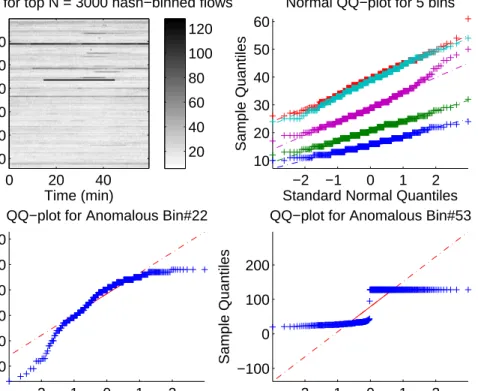
Figure 2.7: Merit Network 16:00-17:00 EST, Aug 1, 2015 – the ‘Tor’ event in Section refsubsec:tor. (Top left) Ingress connectivity for the topN = 3000 hash-binned flows per 10-second windows over 1-hour. (Top-right) QQ-plots demonstrating accuracy of the Normal approximation of typical in-degree distributions. (Bottom plots) QQ-plots for anomalous bins.

LetIt(i) := Pm_j₌₁at(i, j), i= 1, . . . , mbe the in-degree of nodeifor the graphGt.

We wish to find extreme peaks in the values of It(i). Since the hash functions from

(50)

be independent. However in contrast to Sections 2.2.3 and 2.2.4, the counts It(i) are

no longer heavy-tailed but follow normal distribution. This for fixedi randomization by hashing guarantees the independence ofat(i, j)’s inj. The normal approximation

is a direct consequence of CLT when applied to Pm

j=1at(i, j) form sufficiently large. Indeed, Figure 2.6 (top-right plot) shows Normal quantile-quantile plots of It(i), t= 1, . . . , T for 5 typical (non-anomalous) bins i. The linearity in plot supports the assumption of normality. The heatmap shows the entire array (It(i))m×T of in-degrees

computed over 10-second time windows over the duration of 1 hour for N = 3000. The bottom plots in this figure show the QQ-plots corresponding to anomalous bins with high in-degree corresponding to the higher intensity lines in the top-left plot. Clearly these bins are quite off from the normal approximation which suggests that extreme peaks inIt(i) can be used to detect the onset of attacks. Note thatN needs to be large to ensure that CLT works but very large values may meddle with the sparse nature of the matrix At.

We have thus shown that the in degrees It(i), i = 1, . . . , m are independent and identically distributed observations from N(µt, σ_t2). Thus for identifying unusually large in degree values we consider

Dt := max i=1,...,mIt(i),

by the independence of the It(i)’s follows:

P(Dt≤x) = Φ

x−µ_t

σt

m

,

(51)

bin It(i) as anomalous if its values exceeds the threshold

ut(p0)≡u(p0, m, µt, σt) :=µt+σt×p

1/m

0 .

where p0 is the sensitivity parameter controlling for the type I error rate. The em-pirical means and variances of the data serve as reasonably good estimates for the quantities µt and σt. However to reduce their susceptibility to outliers, we use the

EWMA smoothing on the parameters ˆµand ˆσ similar to Step 6 of Algorithm 2.

2.2.6 Detection accuracy

We next describe the detection accuracy of Algorithms 2 and 3 for artificially constructed attacks. Table 2.3 and 2.4 report two metrics, namelyprecision andrecall (Kallitsis et al.(2015)). The data comprises of sketch matrices (databricks) collected at Merit’s Detroit monitoring station usingAMON from an anomaly-free period (one hour during a holiday weekend in July). Attack vectors of varying magnitude (see column three in Tables 2.3 and 2.4) are injected at five randomly chosen points. Three different scenarios are considered: 1) many sources sending traffic to one destination; 2) one source sending traffic to many destinations, and 3) many to many. Each individual experiment is repeated 50 times and we report the average performance in terms of precision and recall. For scenario (3), the input comprises of both destination and source hash binned arrays (see Figure 2.5). The other two scenarios are different where one of destination and source arrays are provided for (1) and (2) respectively. For all situations we allow a grace period of 3 minutes for detection.

Table 2.3 shows the detection accuracy for algorithm 2 for varying values of the pair (p0, λ) = (p, λα) where the best performance was recorded for p = 0.95 and

(52)

p λα Gbps P_d(1) R(1)_d Ps(2) R(2)s Ps(3) R(3)s P_d(3) R(3)_d 0.95 0.50 0.50 0.74 1.00 1.00 0.96 1.00 1.00 0.74 1.00 0.95 0.50 1.50 0.73 1.00 1.00 1.00 1.00 1.00 0.74 1.00 0.95 0.50 2.50 0.73 1.00 1.00 0.98 1.00 1.00 0.74 1.00 0.95 0.60 0.50 0.72 0.93 1.00 0.61 1.00 1.00 0.85 1.00 0.95 0.60 1.50 0.74 0.99 1.00 0.88 1.00 0.99 0.85 0.99 0.95 0.60 2.50 0.73 1.00 1.00 0.92 1.00 1.00 0.85 1.00 0.99 0.50 0.50 1.00 0.73 0.74 0.22 1.00 1.00 1.00 0.99 0.99 0.50 1.50 1.00 0.94 0.98 0.50 1.00 1.00 1.00 1.00 0.99 0.50 2.50 1.00 0.97 1.00 0.71 1.00 0.99 1.00 0.99 0.99 0.60 0.50 0.76 0.24 0.36 0.09 1.00 1.00 1.00 1.00 0.99 0.60 1.50 0.92 0.40 0.08 0.02 1.00 1.00 1.00 1.00 0.99 0.60 2.50 1.00 0.55 0.16 0.04 1.00 1.00 1.00 0.99

Table 2.3: Evaluation of detection Algorithm 2 in Section 2.2.3.

λα = 0.50. The parameterp0 controls for the false alarm rate. The tuning parameter

λis used to robustify the estimation of the tail exponentα (see Algorithm 2). Values of λ close to 1 imply that greater trust is placed on the current estimate of α over the historic ones. This may be disadvantageous when outliers/big spikes are indeed present in the data (large order statistic produce smaller α values). However too much reliability on the past (λ close to 0) makes the algorithm less adaptable to the changes in the traffic.

Table 2.4 illustrates the detection performance of a modification of Algorithm 3, which utilizes EWMA control charts on z-scores, as explained at the end of Section 2.2.4. We employ our methodology for different EWMA pairs (λp, L) =

{(2,0.5),(2,0.6),(3,0.5)} and λ = λα = 0.5. The simulation settings are the same

as that described in the previous paragraph. Best results are obtained for (λp, L) =

(0.60,2). False alarm rates may be controlled with a higherLand/or decrease further