Statistical efficiency in distance sampling

Research Online

Faculty of Engineering and Information Sciences

-Papers: Part A

Faculty of Engineering and Information Sciences

2016

Statistical efficiency in distance sampling

Robert Graham Clark

University of Wollongong, [email protected]

Research Online is the open access institutional repository for the University of Wollongong. For further information contact the UOW Library: [email protected]

Publication Details

Abstract

Distance sampling is a technique for estimating the abundance of animals or other objects in a region, allowing for imperfect detection. This paper evaluates the statistical efficiency of the method when its assumptions are met, both theoretically and by simulation. The theoretical component of the paper is a derivation of the asymptotic variance penalty for the distance sampling estimator arising from uncertainty about the unknown detection parameters. This asymptotic penalty factor is tabulated for several detection functions. It is typically at least 2 but can be much higher, particularly for steeply declining detection rates. The asymptotic result relies on a model which makes the strong assumption that objects are uniformly distributed across the region. The simulation study relaxes this assumption by incorporating over-dispersion when generating object locations. Distance sampling and strip transect estimators are calculated for simulated data, for a variety of overdispersion factors, detection functions, sample sizes and strip widths. The simulation results confirm the theoretical asymptotic penalty in the non-overdispersed case. For a more realistic

overdispersion factor of 2, distance sampling estimation outperforms strip transect estimation when a half-normal distance function is correctly assumed, confirming previous literature. When the hazard rate model is correctly assumed, strip transect estimators have lower mean squared error than the usual distance sampling estimator when the strip width is close enough to its optimal value (± 75% when there are 100 detections; ± 50% when there are 200 detections). Whether the ecologist can set the strip width sufficiently accurately will depend on the circumstances of each particular study.

Disciplines

Engineering | Science and Technology Studies

Publication Details

Clark, R. Graham. (2016). Statistical efficiency in distance sampling. PLoS One, 11 (3), e01492981 -e0149298-24.

Statistical Efficiency in Distance Sampling

National Institute for Applied Statistics Research Australia (NIASRA), University of Wollongong, Wollongong, Australia

*[email protected]

Abstract

Distance sampling is a technique for estimating the abundance of animals or other objects in a region, allowing for imperfect detection. This paper evaluates the statistical efficiency of the method when its assumptions are met, both theoretically and by simulation. The theoret-ical component of the paper is a derivation of the asymptotic variance penalty for the dis-tance sampling estimator arising from uncertainty about the unknown detection parameters. This asymptotic penalty factor is tabulated for several detection functions. It is typically at least 2 but can be much higher, particularly for steeply declining detection rates. The asymptotic result relies on a model which makes the strong assumption that objects are uni-formly distributed across the region. The simulation study relaxes this assumption by incor-porating over-dispersion when generating object locations. Distance sampling and strip transect estimators are calculated for simulated data, for a variety of overdispersion factors, detection functions, sample sizes and strip widths. The simulation results confirm the theo-retical asymptotic penalty in the non-overdispersed case. For a more realistic overdisper-sion factor of 2, distance sampling estimation outperforms strip transect estimation when a half-normal distance function is correctly assumed, confirming previous literature. When the hazard rate model is correctly assumed, strip transect estimators have lower mean squared error than the usual distance sampling estimator when the strip width is close enough to its optimal value (±75% when there are 100 detections;±50% when there are 200 detections). Whether the ecologist can set the strip width sufficiently accurately will depend on the cir-cumstances of each particular study.

1 Introduction

The number of animals in a region is often of ecological importance. This paper considers the distance sampling approach to estimating abundance, in its usual conjunction with line tran-sect sampling. Trantran-sect lines are laid down across a region, often parallel and equally spaced but not necessarily so. Observers move along the transects, and record observations of animals (or plants, or groups of animals, or other objects) and their perpendicular distances from the transect. Empirically, more objects are detected near to transect lines than far from them in many studies, suggesting that detectability is a decreasing function of distance. The distance sampling methodology exploits this phenomenon, by modelling the detection rate as a function OPEN ACCESS

Citation:Clark RG (2016) Statistical Efficiency in Distance Sampling. PLoS ONE 11(3): e0149298. doi:10.1371/journal.pone.0149298

Editor:Shyamal D Peddada, National Institute of Environmental and Health Sciences, UNITED STATES

Received:November 29, 2015

Accepted:January 29, 2016

Published:March 7, 2016

Copyright:© 2016 Robert Graham Clark. This is an open access article distributed under the terms of the

Creative Commons Attribution License, which permits unrestricted use, distribution, and reproduction in any medium, provided the original author and source are credited.

Data Availability Statement:Data are based on simulations. Code to generate the simulated data and figures, etc. is included as supplementary material and is deposited into GitHub (https://github.com/ rgcstats/distance.simulation).

Funding:The author has no support or funding to report.

Competing Interests:The author has declared that no competing interests exist.

of distance. The number of detected objects can then be scaled to estimate the abundanceN

allowing for imperfect detection. Provided the assumptions of the method are met, the maxi-mum range can be made fairly large, thereby increasing the sample size, while avoiding or reducing bias due to declining detection rate. Distance sampling is widely used in ecology: a Web of Science search found 276 articles on distance sampling in ecology journals in 2014 alone. The wide range of applications includes wild horses in the Australian Alps [1], large her-bivores in South Africa’s Kruger National Park [2] and odonata (dragonflies) in a rainforest locality in Papua New Guinea [3]. For a detailed description of the approach, see [4].

The major assumptions of the method are 1. Detection is perfect at zero distance.

2. The detection function is of known form, with some unknown parameters requiring estima-tion. Alternatively, model-averaging may be used provided the detection function is assumed to be one of a known set of alternatives.

3. Animals’distances to the nearest transect line are (at least approximately) uniformly distributed.

It is also assumed that there is no measurement error (for example, false positive detections, or mis-measurement of distances), that there is no movement of objects in response to the observer which could lead to multiple chances of detection, that detection events are indepen-dent, that there are sufficient transects for reliable estimation, and that transect lines are a good representation of the study area. This paper will consider the conventional distance sampling (CDS) scenario where there is only one observer. The same methodology can be used with mul-tiple observers by pooling their detections. Mark recapture and mark recapture distance sam-pling (MRDS) are methods which more fully use data from multiple observers by matching their detections; MRDS, in particular, can be used to relax assumption (i). More recent approaches combine a spatial model with the detection model (see for example [5–7] and [8]). Spatial models allow abundances to be estimated for subregions, and can exploit spatial trends in estimation, however inference may be sensitive to the assumed spatial model which must therefore be carefully constructed. This paper focuses on CDS, as most applications of line transect sampling remain single observer. The use of spatial models in distance sampling is an important advance, but some researchers may decide that the extra effort and complication required to develop an adequate spatial model are not warranted for some studies, particularly when the number of detections is relatively small.

Robustness to the 3 assumptions above is explored in the literature. For example, MRDS can be used to achieve some level of robustness to (i). Assumption (ii) is dealt with by the use of flexible families of detection functions with two or more parameters, and the use of model averaging. [9] argue that (iii) is approximately satisfied provided transect lines are placed ran-domly or systematically from a random starting point. However, [10] question the uniformity assumption and find that CDS estimators are biased in a design-based framework, that is, under repeated random placement of transect lines. The matter remains in contention [11–13]. [11] suggest an alternative approach where the detection function is estimated from a separate calibration study, and [14] propose estimating detection probabilities using multiple observer data and possibly but not necessarily distance data.

A natural alternative to distance sampling is the simple scaling up of observations in a strip about the transect. When strips are too wide, this strip transect estimator is severely negatively biased due to non-detections, particularly of the more distant animals in the strip. When strips are sufficiently narrow, this bias becomes negligible, but the variance of the estimated abun-dance becomes large. Distance sampling aims to achieve lower variance by including

observations at greater distances, while reducing bias by adjusting for non-detection. But there is a hidden cost—the effect of unknown detection parameters on the precision of the estimated abundance—which reverses at least some of the benefit due to wider strips. This paper illumi-nates this cost both asymptotically and in small samples. This existence of a penalty due to unknown detection parameters is known, but no asymptotic expression has been derived in the literature, and the penalty has not been quantified except in a simulation of the half-normal and negative exponential detection functions [15]. A number of authors have compared CDS and strip transect estimators in particular applications (e.g. [1,16]) but typically with only one or two options for strip width. [17] also suggested strip transects as an alternative to CDS but did not make a numerical comparison.

An example of the variability of CDS estimators may be found in [1], which compares strip transect estimates with two different strip widths to CDS estimates with various detection func-tions, and to mark-recapture and MRDS estimates of abundance. Detections of groups of wild horses are attempted up to 200m from a helicopter traversing 91 parallel transect lines in south-eastern Australia, resulting in 52 group detections (pooled from two observers).Table 1

here reproduces results from page 1145 of [1]. The strip transect estimates of abundance are the number of observed groups within 50m or 200m multiplied by the total area divided by the area lying within either 50m or 200m of a transect line, with no allowance for undercount. The values of the Akaike Information Criterion (AIC) are also shown for each detection model. Model averaged estimates are calculated using weights calculated from the AICs as described in [18]. Mark recapture and MRDS results are not reproduced here as they are outside the scope of the current paper. The CDS estimator shown inTable 1corresponds toformula (6)in the next section of the current paper.

Table 1shows that the CDS abundance estimators have high coefficients of variation (CV), with the two-parameter hazard rate model leading to a much higher CV (about 57%) than the other detection models which are one-parameter (CVs between 19% and 25%). The model-averaged estimator has a CV of 30%. The strip transect estimator using detections up to 200m has much lower CV, but is much lower than the CDS estimators, suggesting that it is negatively biased due to undetected groups. The strip transect estimator based on detections up to 50m is more plausible. It is close to the model-averaged CDS estimator, suggesting that its bias is small, presumably because the detection rate would decline relatively little over this shorter range. Surprisingly, the 0–50m strip transect estimator gives similar CVs to the 0–200m model-averaged CDS method, even though it only uses one quarter of the distance range and 44% of the detected groups. This motivated the research in the current paper on the efficiency of CDS estimators.

Section 2 proves for the first time that the usual CDS estimator ofNis also a maximum like-lihood estimator (MLE) ofNunder a particular model provided the likelihood is approximated using Stirling’s Rule. Its asymptotic variance under the model is derived using this result. The asymptotic variance is identical to that of [19], but the use of the Stirling approximation allows a simpler derivation. The limiting variance ofN^is expressed as the variance when the detection function is known multiplied by a penalty for unknownθ. This asymptotic penalty is tabulated for various detection models. It can be substantial, and for many situations arising in practice is between 2 and 6. Section 3 summarizes a simulation study to evaluate the small sample per-formance of CDS estimators for various detection functions and strip transect estimators with differing strip widths. Unlike the theoretical result in Section 2, the simulation allows for over-dispersion in the counts of animals falling in any given range. Section 4 contains conclusions about the magnitude of the penalty due to unknown detection parameters in CDS, and the rela-tive performance of CDS and strip transect estimators.

2 Theoretical results on maximum likelihood estimation of

N

2.1 Notation and background

The aim is to estimate the number of objects, which may be animals, groups of animals or other objects, in a region. LetNbe the number of objects in a defined study area andnbe the number of detections made by an observer moving along predefined line transects. Observa-tion may either be one-sided (only objects to the right, or only objects to the left, are observed) or two-sided. Only objects with perpendicular distance up to a pre-chosen limitwfrom a tran-sect line have a chance of being observed (thecovered region); letNcbe the number of such

objects. Two-sided observation is the more common case, but one-sided observation is some-times necessary, for example if the observer can only see out one side of a vehicle. It is assumed that the probability of observing an object at perpendicular distancedifrom a transect line is

g(di,θ) when 0diw, whereθis a vector ofpparameters specifying the function within a

family. It is assumed thatg(0,θ) = 1 and thatgis a non-increasing function of distance. The

Distancesoftware [20], which implements both CDS and MRDS, allows four possible func-tional forms forg(), including the half-normal model,gðdiÞ ¼ exp

d2_i

y2

, and the hazard rate function,gðdiÞ ¼1 expððdi=y1Þ

y2_{Þ. Both of these functions satisfy theshoulder condition}

thatg0(0) = 0, with the hazard rate model giving greaterflexibility in modelling theshoulder width(i.e. the range near 0 over whichgis relativelyflat). The use of“robust models”, which have enoughflexibility to model a range of typical shapes, is recommended on pages 46–49 of [9], with the hazard rate model given as a particularly useful example.

It is also possible to include other covariates affecting the detectability of objects in the dis-tance function, such as characteristics of the animal or plant (see [21] and [22]).

Letdi,i= 1,. . .,N, be the perpendicular distances from the objects to the nearest transect

line, and letδi= 1 for observed objects andδi= 0 for the rest. Under model assumption (iii)

stated in the Introduction,diare independent and identically distributed uniformU(0,M) for

i= 1,. . .,N, whereMis the maximum possible distance from a transect line. The distribution ofdigivenδi= 1 is easily derived as

gcondðdi;θÞ ¼g dð i;θÞ= Z w

0

g uð ;θÞdu ð1Þ

LetgðθÞ ¼w1R₀wgðu;θÞdube the unconditional probability of detection. (This is the proba-bility that an animal in the covered region is detected, unconditional on its distance, denoted byPain equation (2) of [23]. The notationgðθÞis used here to emphasise that it is the mean

Table 1. Estimates of Density (abundance/area) of Horse Groups obtained from [1].CV is the estimated coefficient of variation of the estimate, given by the square root of the estimated variance divided by the estimate.

Method Detection Function AIC _{Densityd ðN}^_{=AÞ(groups/km}2

) CV%ðN^Þ Strip Width estimated average detection probability

CDS neg. exponential 0.00 0.36 24.8 200m 0.50

CDS uniform (cosine) 0.96 0.28 18.8 200m 0.64

CDS half-normal 1.35 0.28 19.9 200m 0.64

CDS hazard rate 1.87 0.36 57.2 200m 0.50

CDS model-averaged n/a 0.33 30.3 200m 0.55

Strip n/a n/a 0.31 22.1 50m 1.00

Strip n/a n/a 0.18 16.1 200m 1.00

value ofg(di;θ) overdiw.) The conditional likelihood ofds= (d1,. . .,dn)Tgivennis Ld ¼ Yn i¼1 gcondðdi;θÞ ¼ Yn i¼1 g dð i;θÞ ! Z w 0 g u;θ ð Þdu n ¼ Yn i¼1 g dð i;θÞ ! wn_{gð Þθ} n _ð2Þ

and the corresponding conditional log-likelihood givennis

ld ¼ Xn

i¼1

logg dð i;θÞ nlogðgð Þθ Þ nlogw: ð3Þ

The parametersθcan be obtained by setting the derivative ofldwith respect toθto 0. Prior to

this, it is convenient to define

hðu;θÞ ¼ @

@θg uð ;θÞ ð4Þ

andhðθÞ ¼w1R₀whðu;θÞdu. Notice thath(u;θ) is a p-vector wherepis the number of param-eters inθ. The partial derivative ofgðθÞwith respect toθishðθÞ, subject to regularity condi-tions allowing the derivative operator to be taken within the integral. Setting the derivative ofld

to 0 gives the following estimating equation forθ:

0¼X n

i¼1

g dð i;θÞ1hðdi;θÞ ngðθÞ1_hðθÞ ð5Þ

The most commonly used estimator ofNin CDS is: ^

NCDS¼

n Pg ^θ_CML

: _ð6Þ

wherePis the proportion of the area falling within perpendicular distance ofwof a transect line, andθ^_CMLis the solution toEq (5)(CML stands for conditional maximum likelihood, as the likelihoodLdinEq (2)is conditional onn). In CDS, the estimation ofθis model-based and

maximises the likelihood conditional onn, while the estimation ofNinEq (6)is design-based and motivated by the fact thatE½n ¼NPgðθÞ. See equation 1.4 of [9]. See also [23] for a recent discussion of CDS and extensions. The value ofPis assumed to be known, and is approximated in practice by the total length of all transects multiplied byw(and multiplied by 2 for two-sided observation) divided by the region’s area.

Another alternative that has been proposed is maximum likelihood estimation ofN, which is the minimum variance unbiased estimator for large samples subject to regularity conditions. Section 7.2 of [24] derives the likelihood forNandθ. The conditional density ofdsgivennis

LdinEq (2). Under the assumed model,δiare independent Bernoulli random variables with

expected valuegðθÞ. Hence

The likelihood is the product of the probability function ofnandLd: L¼ N n ! fPgðθÞgnf1PgðθÞgnLd ð8Þ ¼ N n ! fPgðθÞgnf1PgðθÞgNn

Y

Y

(See equation 2.33 of [4]).Lcan be maximised with respect toNandθto obtain a maximum likelihood estimator ofN. In this approach, bothNandθare treated as unknown parameters. On pages 16–17, [4] recommend against this approach because in practicenis likely to be over-dispersed and so to have higher variance than implied byEq (7). For example, this would occur if there were positive correlations between the values ofdi. It is worth noting that any such

overdispersion is likely to also invalidateEq (2)and soθ^_CMLandN^CDSto some extent, asEq (2) assumes thatdiare independent conditional onn.

Whenθis known, the MLE ofNis the integer part ofn=ðPgðθÞÞ(see pages 17–19 and 138 of [24]). The same reference also shows that if the factorial terms inEq (10)are approximated using Stirling’s rule andNis treated as a continuous parameter, the MLE is then

^

Nknowny¼n=ðPgð ÞÞθ : ð11Þ

It is straightforward to derive the variance ofN^knownyusing the fact thatnbinðN;PgðθÞÞ:

var N^knowny

¼P2gð Þθ 2varðnÞ ¼NP1gð Þθ 1ð1Pgð Þθ Þ ð12Þ

Whenθis unknown, [19] note that the MLE ofNis the integer part ofn=ðPg θ^ Þwhereθ^is the MLE of these parameters. The next subsection of this paper extends this result by showing thatθ^_CMLandN^CDSmaximise a Stirling approximation to the full likelihoodL. This enables a theoretical result on the large sample variance ofN^_CDS, albeit under the strong assumptionEq (7). The simulation study in Section 3 relaxes this assumption by including overdispersion.

2.2 Derivations of the MLE and its variance based on Stirling

’

s

approximation

The maximum likelihood estimator ofNunder Stirling’s approximation for factorials is

derived in this subsection, where the likelihoodLis given byEq (10). (Note that in section 3.3.1, [9] consider maximization ofLd, notL, to estimateθ, whereLd, defined inEq (2), is the

conditional likelihood givenn). Stirling’s rule log(x!)xlog(x)−ximplies that log N

n

!

¼logfN!=n!ðNnÞ!g ð13Þ

Nlogð Þ N NðnlogðnÞ nÞ fðNnÞlogðNnÞ ðNnÞg ð14Þ

There is a positive probability thatnis equal to 0 orN, in which case log(n) or log(N−n) are not defined. The limit of the right hand side ofEq (15)can easily be shown to equal 0 in these cases, so the following refinement ofEq (15)is used:

log

N n

!

Nlogð Þ N ðNnÞlogðNnÞ nlogðnÞ if 0<n<N

0 if n¼0 or n¼N

( )

:ð16Þ

Lwill be maximised with respect toNandθtreatingNas a continuous parameter. Stirling’s

approximation for log(x!) is very accurate even for smallxas long asxis at least 2 or 3, and bothN−nandnwould be well above this in practice. Theorem 1 states the MLEs and the approximate Fisher information.

Theorem 1The model defined by Eqs (1) and (7) is assumed, and it is assumed that the log of the likelihoodEq (10)can be approximated usingEq (16), leading to

l ¼ Nlogð Þ N ðNnÞlogðNnÞ nlogðnÞ þnlogðPÞ nlogðwÞ

þðNnÞlogð1Pgð ÞθÞ þX

n

i¼1

logðg dð i;θÞÞ ð17Þ

LetObe an open set defining the set of feasible values ofθ. If there is a uniqueθ^_CMLsatisfying

Eq (5)then it is the maximum likelihood estimator, and the MLE of N on(0,1)isN^CDSin

Eq (6).

Let D be a random variable with density gðdÞ=R₀wgðuÞdu for0dw,which is also the dis-tribution of diconditional on detection. The Fisher Information of(N,θT)Tis approximately

equal to IðN;θÞ INN I T Ny INy Iyy 2 4 3 5 ð18Þ

for large N, where

INN ¼ N1ð1Pgð Þθ Þ 1_{Pgð Þθ ð19Þ} Iyy ¼ NPw1 Rw 0 hðu;θÞhðu;θÞ T g uð ;θÞ1duþNPhð Þθ hð Þθ Tð1Pgð Þθ Þ1 ð20Þ ¼ NPgð Þθ varDðhðD;θÞ=g Dð ;θÞÞ þNPhð Þθhð Þθ T gð Þθ 1ð1Pgð Þθ Þ1 ð21Þ INy ¼ ð1PgðyÞÞ 1 PhðyÞ ð22Þ

Surprisingly,θ^_CMLandN^CDSmaximise the Stirling approximation to the full likelihoodL, even thoughθ^_CMLwas defined as the maximizer of the conditional likelihoodLdgivenn(notL),

andN^CDSwas motivated by a design-based argument.

LetVbe the inverse of the Fisher Information matrix inEq (18). Subject to regularity condi-tions, maximum likelihood estimators are asymptotically normal with expectation equal to the true parameter values and variance-covariance matrix equal to the inverse of the Fisher Infor-mation matrix. Unfortunately these regularity conditions do not hold here, for example condi-tion (M3) of the Central Limit Theorem on pages 499–500 of [25] is not met, becausenandds

are dependent. Moreover,Eq (18)is only the approximate Fisher information based on a Taylor Series expansion, whereas the usual Central Limit Theorem requires the exact Fisher

information. [26] uses an alternative method of proof to derive a Central Limit Theorem for the MLE. It is shown in this working paper thatVis indeed the limiting variance ofðN^;θ^TÞT_. The proof in [26] is essentially a simplified version of the proof of the result in [19] which does not use the Stirling approximation. Theorem 1 is an advance on the result in [19], because it shows thatN^CDSis the full maximum likelihood estimator (subject to the Stirling approxima-tion), and also provides a simpler derivation ofV. Theorem 1 helps explain thefinding of [19] that the difference betweenN^CDSand the exact maximum likelihood estimator (i.e. the MLE when the Stirling approximation is not made) is small asymptotically. The theorem also sug-gests that there is no need for the calculation of the exact MLE in practice, even when the model assumptions are justified, sinceN^CDSmaximises an excellent approximation to the full likelihood.

It is convenient to expressVin block form. We will henceforth mostly writeg(u),h(u),g

andhfor readability, rather thang(u;θ) etc. Using a standard result on the inverse of a matrix in block form (e.g. 5.16a of [27]),Vis equal to

V¼ V₁₁ VT 21 V₂₁ V₂₂ " # ð23Þ where V22 ¼ IyyINyI 1 NNI T Ny 1 ¼N1P1D1g1 V11 ¼ Iyy1þIyy1ITNyV22INy ¼ Nð1PgÞP1g1þNP1g3hT_D1_h V₂₁ ¼ VT 21¼ V22INyINN1 ¼ g2P1D1h 9 > > > > > > > > > > > = > > > > > > > > > > > ; ð24Þ

andΔis thepbypmatrix defined by

D¼varD½hð ÞD =g Dð Þ: ð25Þ

The limiting variance ofN^CDS,V11fromEq (24), is of primary interest. It can be expanded

by elementary operations as var N^CDS ¼V₁₁¼var N^knowny F ð26Þ

where var N^knowny

is the variance ofN^ whenθis known, as defined byEq (12), and

F¼1þhTD1hg2ð1PgÞ1 ð27Þ

is a penalty term attributable toθrequiring estimation. The penaltyFis always 1 or greater, becauseΔis a variance-covariance matrix, and so is positive semi-definite.

The coefficient of variance (CV) ofN^CDSfollows directly, noting thatE½n ¼NPg:

CV2 ¼ var N^CDS

=N2¼FNP1g1ð1PgÞ=N2 ð28Þ

2.3 Numerical values of the asymptotic variance for selected models

D¼w1 Rw 0 hðuÞhðuÞ T gðuÞ1du g hhT g2 ð30Þ

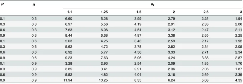
and calculating by quadrature using theintegratefunction in the R Statistical Environment [28].Table 2shows values ofFnumerically calculated for various hazard rate models. The parameterθ2determines the shape of the detection curve, with 1.1 giving a very narrow

shoul-der (i.e. steeply declining for small distances) and 3 giving a very wide shoulshoul-der. Hazard rate detection models for a number of values ofθ2are illustrated in the next section. The parameter

θ1is calculated numerically to give the specifiedg in each row.

Table 2shows thatFincreases asθ2decreases, i.e. as the shoulder becomes narrower. For a

giveng,Fdecreases as the coverage ratePincreases. This is because increasingPimproves the precision ofN^CDS, but it improves the precision ofN^knownyeven faster. For a givenP,Fdecreases

asgincreases whenθ22 (narrow shoulder), but increases asgincreases whenθ2>2. A

pos-sible reason is that whenθ2is small andgis large, the detection function is near 1 for much of

its range but then decreases precipitously. The fact that it remains near 1 for much of the range may mean thatN^is relatively insensitive to^θ. In contrast, whenθ2>2 andgis large, the

detection function declines more smoothly, so thatN^CDSis more sensitive toθ^.

Values ofgof 0.1, 0.3 or 0.6,P= 0.3 andθ21.25 are probably the most representative of

studies in practice.Fvaries from 1.9 to 5.6 in this subset ofTable 2.

Table 3shows similar results for half-normal detection models. The values ofFare gener-ally much closer to 1 than inTable 2, varying from 1.5 to 1.9 in the subset of the table where

g 2 f0:1;0:3;0:6gandP= 0.3.Fincreases withP, as inTable 2.Fincreases withg forfixedP, similar to the wide-shouldered results inTable 2whereθ2>2.

3 Simulation study

3.1 Design of the simulation study

Generation of distancesdifori= 1,. . .,N. Distance data are simulated for abundancesN

such that the expected numbers of detections areE[n] = 50, 100, 200,. . ., 1000, and the fraction of the area covered isP= 0.1. 10,000 simulations are used in every case.

Distancesdiare generated both with and without overdispersion. In the latter case,diare

independentU(0, 10) random variables. The maximum range of observation is set tow= 1, so that objects are only eligible for detection whendi1, and so the probability of any given

object falling within the covered area isP= 0.1. One implication of this model is that the num-ber of objectsn(v) with distance falling into any given interval of lengthvwithin [0, 10] is dis-tributed asn(v)*bin(N,vP), and henceE[n(v)] =NvPandvar[n(v)] =NvP(1−vP). For example,Ncis a special case ofn(v) withv= 1. The assumption of independent uniform

dis-tances has been criticised because in practicen(v) is often observed to be overdispersed, with variance greater thanNvP(1−vP).

Overdisperseddiare generated by firstly replacing theU(0, 10) distribution by the discrete

approximation with probability 0.001 at each of 1000 evenly spaced values between 0 and 10. The probability thatdifalls in any given interval would then be 0.001 in the non-overdispersed

case. Overdisperseddiare assumed to be discrete random variables with the same set of

possi-ble values, with probabilityϕkfor valuek= 1,. . ., 1000. The vectorϕis simulated as coming

from a Dirichlet distribution with vector parameter equal to 0.001α11000where11000is a vec-tor containing 1000 values all equal to 1, andαis a parameter which controls the variance ofϕ.

Whenα! 1,ϕis equal to11000/1000 with probability 1, resulting in the non-overdispersed case. For 0<α<1,ϕare random variables each lying between 0 and 1, withP1000_{k¼1 k}¼1. The parametersϕare generated anew for each simulation, and {di:i= 1,. . .,N} are then generated

as independent discrete random variables with probabilitiesϕat each of the 1000 evenly spaced values between 0 and 10.

The overdisperseddihave the property thatn(v) is beta-binomial distributed with

parame-tersN,αPv, andα(1−Pv). (This follows from the properties of the Dirichlet-multinomial and beta-binomial distributions—see for example [29].) The expected value ofn(v) is thenNvPas before, but the variance is inflated tovar[n(v)] =cNvP(1−vP) wherec= (α+N)/(α+ 1) is an overdispersion factor. Values ofαcorresponding toc= 1, 2 and 3 are used.

The above process is a discrete approximation of a Dirichlet process with base distribution given byU(0, 10). Dirichlet processes are widely used as prior distributions for distribution functions (e.g. chapter 23 of [30]). This also makes them suitable to simulate overdispersed

Table 2. Asymptotic penalty (F) for the hazard rate model for selected values of the coverage rateP, the shape parameter (_θ2) and the mean

detec-tion rateg.The largest distance for which detection is attempted isw= 1 in all cases.

P g θ2 1.1 1.25 1.5 2 2.5 3 0.1 0.3 6.60 5.28 3.99 2.79 2.25 1.94 0.3 0.3 6.97 5.56 4.19 2.91 2.33 2.00 0.6 0.3 7.63 6.06 4.54 3.12 2.47 2.11 0.9 0.3 8.44 6.68 4.97 3.38 2.65 2.25 0.1 0.6 5.03 4.25 3.43 2.59 2.17 1.92 0.3 0.6 5.62 4.72 3.78 2.82 2.34 2.05 0.6 0.6 6.92 5.77 4.56 3.33 2.71 2.34 0.9 0.6 9.23 7.63 5.96 4.24 3.38 2.87 0.1 0.9 3.28 2.93 2.54 2.09 1.85 1.70 0.3 0.9 3.85 3.41 2.91 2.36 2.06 1.87 0.6 0.9 5.52 4.82 4.04 3.16 2.69 2.39 0.9 0.9 11.94 10.25 8.35 6.24 5.08 4.35 doi:10.1371/journal.pone.0149298.t002

Table 3. Asymptotic penalty (F) for the half-normal model for selected values of the coverage rateP and the mean detection rateg.The largest distance for which detection is attempted isw= 1 in all cases.

P g Penalty (F) 0.1 0.3 1.52 0.3 0.3 1.55 0.6 0.3 1.61 0.9 0.3 1.69 0.1 0.6 1.78 0.3 0.6 1.90 0.6 0.6 2.15 0.9 0.6 2.60 0.1 0.9 2.23 0.3 0.9 2.54 0.6 0.9 3.44 0.9 0.9 6.90 doi:10.1371/journal.pone.0149298.t003

data, particularly as the resultingdihave the property that the number of distances falling in

any interval is overdispersed to the same degree.

Simulation of detection process. Objects are detected with probabilityg(di;θ) when

diw= 1 for eachi, with detection independent across objects. Two families of detection

func-tions are used: the hazard rate and the half-normal. Both are among those proposed in [9]. The two-parameter hazard rate function meets the requirement specified on page 41 of [9] of being a flexible model, giving some robustness to mis-specified detection function; in particular, it allows the shoulder to be narrow or wide. The half-normal detection function is less flexible, but is also often used, and would generally be easier to fit from data as it has only one parameter.Fig 1shows the 4 particular distance functions used: hazard rate (hr) functions

gðdi;θÞ ¼1eðdi=y1Þy2_withθ_{= (0.405, 1.25),}θ_{= (0.448, 2) and}θ_{= (0.484, 3) corresponding}

to a very narrow, narrow, and wide shoulder respectively; and a half-normal (hn) function

gðdi;θÞ ¼1eðdi=yÞ2=2_withθ_{= 0.502. This gives a variety of shapes of the detection function,} with all 4 having the same average detection rate ofgðθÞ ¼0:6. This means that the number of detections is approximatelynPgðθÞN ¼0:06N. The values ofg(w) for all three functions are at least 0.11, and all but the wide hazard rate function are at least 0.14, roughly in line with the rule of thumb for choice ofwon page 16 of [9]. Thefigure also shows the asymptotic pen-altyFdue to unknownθfor each detection function. The penalty ranges from 2 to 5.4.

Estimators of abundance. The CDS estimatorN^CDSdefined inEq (6)is calculated using the hazard rate model and the half-normal model. The CDS estimator assuming knownθ, defined inEq (11), is also calculated. This last option is of course unrealistic in practice, but is included to show the impact of uncertainty aboutθ.

An estimate ofNis also calculated using the strip transect estimatorN^ST ¼n=P. This is unbiased under the binomial modeln*bin(N,P), which incorrectly assumes perfect detection up to distancew. The strip transect estimator is also applied to restricted datasets using only those distances up to a range ofw0= 0.01, 0.02,. . ., 1, withN^STðw0Þ ¼n½dw0=ðPw0=wÞ.

Each simulation corresponds to a single detection function, and a single value ofE[n] and of

c. 10,000 populations of distances and detections are generated in each simulation. All compu-tations are carried out in the R statistical environment version 3.0.1 [28]. TheDistance

package [31] is not used because of occasional non-convergence (this would generally not be an issue in practice, but is a problem in a large simulation). The estimatorθ^_CMLis calculated by maximisingldfromEq (3)using theoptimfunction, using the Nelder-Mead method for the

two-parameter hazard rate function and the Brent method for the one-parameter half-normal function. The complete simulation requires approximately 14 hours on a Macbook Pro with a 2.7GHz Intel Core i7 processor and 16GB of RAM. The code to conduct the simulation and produce thefigures and tables is inS1 Code.

The aim of the simulation is to estimate the penalty factor due to unknown detection parameters for finite sample sizes, and to compare the mean squared errors (MSEs) of line transect and strip transect estimators in different scenarios. The focus of the paper is on vari-ances and mean squared errors of abundance estimators, so variance estimators and confidence interval coverage are not reported on.

3.2 Simulation results for the asymptotic penalty

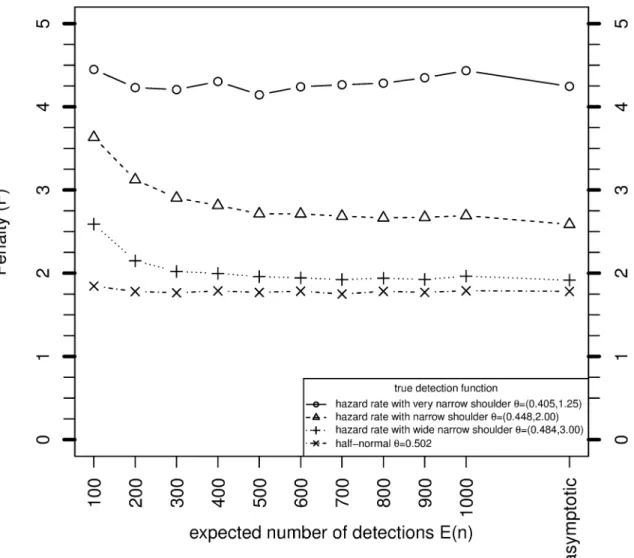
Fig 2shows how the simulation estimates ofFconverge to the asymptotic values asnandN

increase, forc= 1. For the hazard rate with very narrow shoulder and the halfnormal model, the asymptotic approximation is good even forE[n] = 100. For the other two models, the small sample penalties are higher than the asymptotic value forE[n] = 100, but converge to the

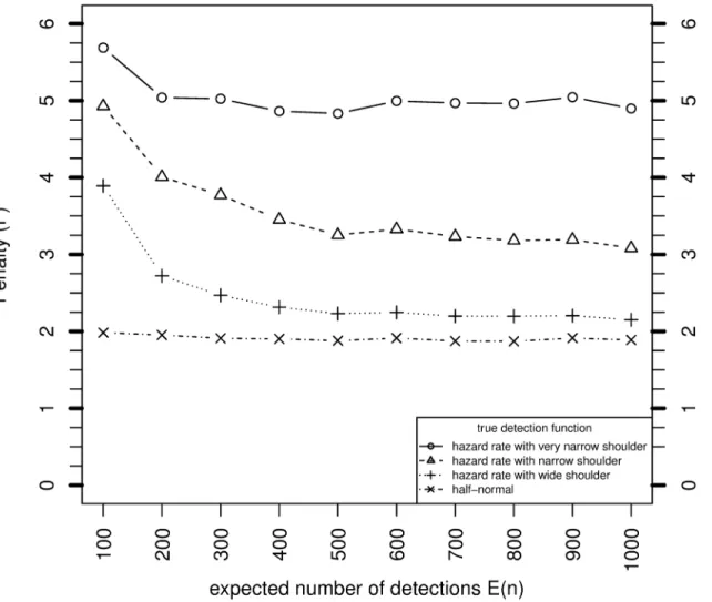
asymptote asE[n] increases. The results provide a computational confirmation of the deriva-tion ofFin Section 3.Fig 3shows the simulation estimates ofFwhen the overdispersion parametercis 2. No asymptotic result forFis available in this case. The values ofFare 0.1–0.7 higher than whenc= 1.

3.3 Simulation MSEs of CDS and strip transect estimators

Fig 4compares the simulation MSEs ofN^CDS, andN^STwith varying strip width, whenE[n] = 50. The 3 horizontal red lines in each plot are the MSEs ofN^CDS, which make use of all detections up to distancew= 1. The 3 lines are for overdispersion values ofc= 1, 2 and 3. The 3 blue curves show the MSEs ofN^STforc= 1, 2 and 3, with strip widths of 0.01, 0.02,. . ., 1.Fig 4(a)shows MSEs for the half-normal detection function.Fig 4(b), 4(c) and 4(d)are results for the hazard rate models with very narrow, narrow and wide shoulders, respectively.

The format ofFig 4is loosely based on Figure 1 in [15]. [15] compared CDS and strip tran-sect estimators for the half-normal and negative exponential detection functions (both one parameter families) forn= 40, 60 and 100, andc= 1, 2 and 3. Here we extend these results to the two-parameter hazard rate function, and we simulate over-dispersed distances correspond-ing toc= 1, 2 and 3, rather than using the approximate formula in [15] to convert results when

c= 1 to other values ofc.

Figs5,6and7are of the same format asFig 4and show results whenE[n] is 100, 200 and 400 respectively.

For the half-normal function, Figs4–7replicate the finding of [15] that CDS dominates strip transect estimators, with the former having lower MSE for almost all values ofc,E[n] and strip width.

Fig 1. Detection Functions used to Generate Simulated Data.The variance penalty factorsFfromEq (26)due to unknownθare also shown.

For the hazard rate function, the picture is quite different, presumably because of the larger value of the penalty (F) due to unknown detection parameters for this model. [15] argue that

c= 2 is the most practically relevant scenario out ofc= 1, 2 and 3, so we concentrate on this case. For this value ofc, and for the narrow shoulder detection function (panel (c) of each fig-ure),N^SThas lower MSE thanN^CDSwhen the strip width is 0.1 and above (whenE[n] = 50), between 0.15 and 0.71 (whenE[n] = 100), 0.19 and 0.54 (whenE[n] = 200) and 0.21 and 0.45 (whenE[n] = 400). The optimal strip widths are 0.47, 0.42, 0.38 and 0.35 forE[n] equal to 50, 100, 200 and 400, respectively.

^

NCDSperforms better relative toN^STthan the above when the hazard rate function has a wide shoulder, and worse than the above when the shoulder is very narrow.

The MSEs of bothN^CDSandN^STincrease ascincreases, particularlyN^ST. So whencincreases,

MSE½N^CDS=MSE½N^STdecreases slightly.

Simulations were also carried out with values ofPother than 0.1. Results forPequal to 0.2, 0.25, 0.3 and 0.5, withE[n] = 100, are inS1,S2,S3andS4Figs, respectively. A comparison of

Fig 2. Variance of MLE ofNwhenθis unknown relative to when it is known, for various sample sizes based on simulation, and asymptotically fromEq (26), whereP= 0.1,c= 1 andg¼0:6.

these figures toFig 4shows that mean squared errors decrease slightly asPincreases. The rela-tive performance of the different methods for the variouscandwis insensitive toP.

4 Conclusions

To achieve a given coefficient of variationCVfor the line transect estimator, the required expected sample size is

E½n ¼ðN1þCV2F1Þ1 ð31Þ

(follows from rearrangingEq (29)). Whennis much smaller thanN, this simplifies to

E½n ¼F=CV2: ð32Þ

The factorFis the inflation due to unknown detection function parameters. Asymptotic values

ofFare made available here for thefirst time (see Tables2and3), albeit under a strong simpli-fying assumption that counts are binomially distributed. The asymptotic values ofFfor typical hazard rate models are between 2 and 6. Simulation confirms the accuracy of the asymptotic result when there is no overdispersion, and shows thatFis larger in the presence of

Fig 3. Variance of MLE ofNwhen_θis unknown relative to when it is known, for various sample sizes based on simulation, and asymptotically fromEq (26), whereP= 0.1,c= 2 andg¼0:6.

overdispersion. TheRpackagedistance.sample.size[32] calculatesFand required sample size using the methods described in the current paper.

Note that the inflation factorFdoes not apply ifgis modelled using mark-recapture data as suggested by [14].

Fig 4. Relative root mean squared errors (RRMSE) (%) of CDS and strip transect estimators estimators (strip widths ranging from 0 to 1) ofN, for 4 detection functions, withE[n] = 50,P= 0.1 andg¼0:6.

The results onFhelp to explain the relative mean squared errors of strip and CDS estima-tors in the simulation. When the number of detectionsnis sufficiently large (e.g. 400), CDS outperforms strip transect estimation unless the strip width is moderately close to its optimal value (within about ± 25%). This is because variances of estimated abundances are then

Fig 5. Relative root mean squared errors (RRMSE) (%) of CDS and strip transect estimators estimators (strip widths ranging from 0 to 1) ofN, for 4 detection functions, withE[n] = 100,P= 0.1 andg¼0:6.

relatively small, so that bias considerations are paramount. For smallern, the variance of the CDS estimator becomes more dominant, partly due to the penaltyF. As a result, when the overdispersion factor is 2 and the hazard rate model applies, we find that strip transects give lower mean squared error (MSE) than CDS when:

Fig 6. Relative root mean squared errors (RRMSE) (%) of CDS and strip transect estimators estimators (strip widths ranging from 0 to 1) ofN, for 4 detection functions, withE[n] = 200,P= 0.1 andg¼0:6.

• n= 50 and the strip width is 0.1 or higher (with an optimal width of about 0.4), where a width of 1 corresponds to a typical detection range for distance sampling;

• n= 100 and the strip width is between 0.2 and 0.7, i.e. within about ± 75% of its optimal value of 0.42; or

Fig 7. Relative root mean squared errors (RRMSE) (%) of CDS and strip transect estimators estimators (strip widths ranging from 0 to 1) ofN, for 4 detection functions, withE[n] = 400,P= 0.1 andg¼0:6.

• n= 200 and the strip width is within about 50% of its optimal value.

A Dirichlet process approach was able to generate non-uniform detections resulting in over-dispersion factors of 1, 2 and 3. This approach has not been used in simulations in statistical ecology to the author’s knowledge. It would be applicable to any simulation where overdisper-sion or robustness relative to an assumed spatial model is of interest.

The simulation settings are more favourable to CDS than to strip transect estimators. In particular, it is assumed that the functional form used in CDS estimation matches the true detection function. This assumption will never be perfectly justified in reality, and its failure will impact on the performance of CDS estimators to some extent. Model selection or model averaging are often used to try to identify the correct model, but uncertainty about the model form will inflate variances and potentially lead to some bias as well. In contrast, strip transect estimators do not require a specification of the detection function. Of course, the properties of strip transect estimators depend on the mean detection rate in the strip, but beyond that there is no particular impact of one functional form rather than another. The simulations withc= 1 are also favourable to both CDS and strip transects as they mean that distances are independent and uniformly distributed. This is relaxed to some extent by the overdispersed simulations withcequal to 2 and 3, however the Dirichlet process used is still centred on the uniform distri-bution. When there is a more severe departure from uniformity, CDS estimators will be biased, and strip transect estimators will also be affected to some degree.

The choice of methodology for assessing abundance, as well as the determination of required sample size, should be informed by consideration of all relevant biases and by the likely achievable precision. The results in this paper will help in this process, by providing a sample size formula reflecting the penalty due to unknown detection parameters, theoretical and simulation results on the size of this penalty, and a comparison of the mean squared errors of strip and line transect estimators in a wide-ranging simulation.

Appendix: Proof of Theorem 1

ApplyingEq (15), we approximatel= log(L) by

l Nlogð Þ N ðNnÞlogðNnÞ nlogðnÞ þðNnÞlogð1Pgð Þθ Þ

þnlogðPÞ nlogðwÞ þX

n

i¼1

logg dð i;θÞ ð33Þ

The next step is to differentiatelto obtain the score function:

@l

@N ¼ NN

1_{þ1 logð Þ N ðNnÞ ðNnÞ}1 _{logðNnÞ þlogð1Pgð Þθ Þ ð34Þ} ¼ logð Þ N logðNnÞ þ logð1Pgð Þθ Þ ð35Þ

@l

@θ ¼

Xn i¼1

g dð i;θÞ1hðdi;θÞ ðNnÞð1Pgð Þθ Þ1Phð Þθ ð36Þ

The MLE is obtained by setting Eqs (35) and (36) to 0. Firstly, setEq (35)to 0 and expo-nentiate both sides:

which leads directly to

^

N ¼n= Pg ^θ

n o

: ð38Þ

SettingEq (36)to 0, and then substituting forN^fromEq (38)gives an estimating equation for

θ: 0 ¼ X n i¼1 g dð i;θÞ 1_{hðdi;θÞ N^nð1Pgð Þθ Þ}1_{Phð Þθ ð39Þ} ¼ X n i¼1 g dð i;θÞ1hðdi;θÞ nP1gð Þθ 1nð1Pgð Þθ Þ1Phð Þθ ð40Þ ¼ X n i¼1 g dð i;θÞ 1 hðdi;θÞ nP1gð Þθ 1ð1Pgð Þθ Þð1Pgð Þθ Þ1Phð Þθ ð41Þ ¼ Xn i¼1 g dð i;θÞ 1_h di;θ ð Þ ngð Þθ 1hð Þθ ð42Þ

Results Eqs (38) and (42) give the Theorem result on the maximum likelihood estimators of

Nandθ.

The Fisher Information is given by the variance of the score vector, the elements of which are given by Eqs (35) and (36). It can be written as

IðN;θÞ ¼ INN I T Ny INy Iyy 2 4 3 5¼ varð@l=@NÞ covð@l=@N; @l=@θÞ T covð@l=@N; @l=@θÞ varð@l=@θÞ 2 4 3 5_: ð43Þ

The block elements ofIare easily derived. Some preliminary notes:

1. LetDbe a random variable with densitygðd;θÞ=R₀wgðu;θÞdufor 0dw. 2. The distancesdifollow the same distribution asD, conditional onn.

For the remainder of the proof, I will writeg(u),h(u),gandhfor readability, rather than

g(u;θ) etc. Using (a), (b) and (c), we obtain:

Iyy ¼ varð@l=@θÞ ¼E varf ð@l=@θjnÞg þvar Ef ð@l=@θjnÞg ð44Þ

¼ Eðnvarðhð ÞD =g Dð ÞÞÞ þvarnhg1ðNnÞð1PgÞ1Ph ð45Þ

¼ E½nvarðhðDÞ=gðDÞÞ þvarnhg1ð1PgÞ1ð1PgþPgÞ þconst:

ð46Þ ¼ E½nvarðhðDÞ=gðDÞÞ þvarnhg1ð1PgÞ1 ð47Þ ¼ NPgvarðhðDÞ=gðDÞÞ þvarð Þn hhTg2ð1PgÞ2 ð48Þ ¼ NPgvarðhðDÞ=gðDÞÞ þNPgð1PgÞhhTg2ð1PgÞ2 ð49Þ ¼ NPgvarðhðDÞ=gðDÞÞ þNPhhTg1ð1PgÞ1 ð50Þ INy ¼ covð@l=@N; @l=@θÞ ð51Þ ¼ Ecovð@l=@N; @l=@θjnÞ þcov Ef ð@l=@NjnÞ;Eð@l=@θjnÞg ð52Þ ¼ 0cov log ðNnÞ;ng1hþnð1gÞ1h ð53Þ ¼ g1ð1gÞ1hcov logf ðNnÞ;ng ð54Þ

AsN! 1n!pNPg, so the right hand side ofEq (54)can be approximated using afirst order Taylor Series ofnaboutE½n ¼NPg:

INy g1ð1PgÞ 1 Ph cov log ðNNPgÞ ðNNPgÞ1ðnNPgÞ;n ð55Þ ¼ g1ð1PgÞ1hN1ð1PgÞ1varðnÞ ð56Þ ¼ g1ð1PgÞ2hN1NPgð1NPgÞ ð57Þ ¼ ð1PgÞ1Ph ð58Þ

n¼Ng:

INN ¼ varð@l=@NÞ ¼var logð ðNnÞÞ ð59Þ varlogðNNPgÞ þðNNPgÞ1ðnNPgÞ ð60Þ

¼ N2ð1PgÞ2varðnÞ ð61Þ

¼ N2ð1PgÞ2NPgð1PgÞ ð62Þ

¼ N1ð1PgÞ1Pg ð63Þ

Supporting Information

S1 Fig. Simulation results for P = 0.2 with E[n] = 100.

(EPS)

S2 Fig. Simulation results for P = 0.25 with E[n] = 100.

(EPS)

S3 Fig. Simulation results for P = 0.3 with E[n] = 100.

(EPS)

S4 Fig. Simulation results for P = 0.5 with E[n] = 100.

(EPS)

S1 Code. R program used to produce simulation results.

(R)

Acknowledgments

I am grateful to Geoff Robertson and Michelle Dawson who provided background on sampling of brumbies and to Alan Welsh for his insights and encouragement. Anonymous referees made comments which improved the paper. All views are the author’s own.

Author Contributions

Conceived and designed the experiments: RC. Performed the experiments: RC. Analyzed the data: RC. Contributed reagents/materials/analysis tools: RC. Wrote the paper: RC.

References

1. Walter MJ, Hone J. A comparison of 3 aerial survey techniques to estimate wild horse abundance in the Australian Alps. Wildlife Society Bulletin. 2003;p. 1138–1149.

2. Kruger J, Reilly B, Whyte I. Application of distance sampling to estimate population densities of large herbivores in Kruger National Park. Wildlife Research. 2008; 35(4):371–376. doi:10.1071/WR07084

3. Oppel S. Using distance sampling to quantify Odonata density in tropical rainforests. International Jour-nal of Odonatology. 2006; 9(1):81_–88. doi:10.1080/13887890.2006.9748265

4. Buckland ST, Anderson DR, Burnham KP, Laake JL, Borchers DL, Thomas L. Advanced Distance Sampling. Oxford: Oxford University Press; 2004.

5. Hedley SL, Buckland ST. Spatial models for line transect sampling. Journal of Agricultural, Biological, and Environmental Statistics. 2004; 9(2):181–199. doi:10.1198/1085711043578

6. Johnson DS, Laake JL, Ver Hoef JM. A model-based approach for making ecological inference from distance sampling data. Biometrics. 2010; 66(1):310–318. doi:10.1111/j.1541-0420.2009.01265.x PMID:19459840

7. Miller DL, Burt ML, Rexstad EA, Thomas L. Spatial models for distance sampling data: recent develop-ments and future directions. Methods in Ecology and Evolution. 2013; 4(11):1001–1010. doi:10.1111/ 2041-210X.12105

8. Oedekoven C, Buckland S, Mackenzie M, King R, Evans K, Burger L Jr. Bayesian methods for hierar-chical distance sampling models. Journal of Agricultural, Biological, and Environmental Statistics. 2014;p. 1–21.

9. Buckland S, Anderson D, Burnham K, Laake J, Borchers D. Introduction to Distance Sampling: Estimat-ing Abundance of Biological Populations. Oxford: Oxford University Press; 2001.

10. Barry SC, Welsh A. Distance sampling methodology. Journal of the Royal Statistical Society: Series B (Statistical Methodology). 2001; 63(1):23_–31. doi:10.1111/1467-9868.00274

11. Melville G, Welsh A. Line transect sampling in small regions. Biometrics. 2001; 57(4):1130–1137. doi: 10.1111/j.0006-341X.2001.01130.xPMID:11764253

12. Fewster RM, Laake JL, Buckland ST. Line transect sampling in small and large regions. Biometrics. 2005; 61(3):856–859. doi:10.1111/j.1541-0420.2005.00413_1.xPMID:16135038

13. Melville GJ, Tracey JP, Fleming PJ, Lukins BS. Aerial surveys of multiple species: critical assumptions and sources of bias in distance and mark–recapture estimators. Wildlife Research. 2008; 35(4):310– 348. doi:10.1071/WR07080

14. Melville GJ, Welsh AH. Model-based prediction In ecological surveys including those with incomplete detection. Australian & New Zealand Journal of Statistics. 2014; 56(3):257–281. doi:10.1111/anzs. 12084

15. Burnham KP, Anderson DR, Laake JL. Efficiency and bias in strip and line transect sampling. The Jour-nal of Wildlife Management. 1985;p. 1012–1018. doi:10.2307/3801387

16. Azhar B, Zakaria M, Yusof E, Leong PC. Efficiency of fixed-width transect and line-transect-based dis-tance sampling to survey red junglefowl (Gallus gallus spadiceus) in Peninsular Malaysia. Journal of Sustainable Development. 2009; 1(2):63–73. doi:10.5539/jsd.v1n2p63

17. Welsh A. Incomplete detection in enumeration surveys: whither distance sampling? Australian & New Zealand Journal of Statistics. 2002; 44(1):13_–22. doi:10.1111/1467-842X.00204

18. Burnham KP, Anderson DR. Model Selection and Multi-Model Inference: A Practical Information-Theo-retic Approach. New York: Springer-Verlag; 2002.

19. Fewster R, Jupp P. Inference on population size in binomial detectability models. Biometrika. 2009; 96 (4):805–820. doi:10.1093/biomet/asp051

20. Thomas L, Buckland ST, Rexstad EA, Laake JL, Strindberg S, Hedley SL, et al. Distance software: design and analysis of distance sampling surveys for estimating population size. Journal of Applied Ecology. 2010; 47(1):5–14. doi:10.1111/j.1365-2664.2009.01737.xPMID:20383262

21. Marques FF, Buckland ST. Incorporating covariates into standard line transect analyses. Biometrics. 2003; 59(4):924–935. doi:10.1111/j.0006-341X.2003.00107.xPMID:14969471

22. Marques TA, Thomas L, Fancy SG, Buckland ST, Handel C. Improving estimates of bird density using multiple-covariate distance sampling. The Auk. 2007; 124(4):1229_–1243. doi:10.1642/0004-8038 (2007)124%5B1229:IEOBDU%5D2.0.CO;2

23. Buckland ST, Oedekoven CS, Borchers DL. Model-based distance sampling. Journal of Agricultural, Biological, and Environmental Statistics. 2015;p. 1_–18.

24. Borchers DL, Buckland ST. Estimating Animal Abundance: Closed Populations. London: Springer-Verlag; 2002.

25. Lehmann EL. Elements of Large-Sample Theory. New York: Springer; 1999.

26. Clark RG. Efficiency and Robustness in Distance Sampling; 2015. National Institute for Applied Statis-tics Research Australia (NIASRA) Working Paper 15_–15. Available from:http://niasra.uow.edu.au/ publications/UOW185981.html.

27. Harville DA. Matrix Algebra from a Statistician’s Perspective. New York: Springer; 1997.

28. R Core Team. R: A Language and Environment for Statistical Computing. Vienna, Austria; 2013.http:// www.R-project.org/.

29. Johnson NL, Kotz S, Balakrishnan N. Discrete Multivariate Distributions. Wiley New York; 1997.

31. Miller DL. Distance: a simple way to fit detection functions to distance sampling data and calculate abundance/density for biological populations; 2014. R package version 0.9. Available from:http:// CRAN.R-project.org/package=Distance.

32. Clark RG. distance.sample.size: Calculates study size required for distance sampling; 2016. R pack-age version 0.0. Available from:http://CRAN.R-project.org/package=distance.sample.size.