Uncovering exceptional predictions using exploratory analysis of second stage machine learning.

(1)

University of Louisville University of Louisville

ThinkIR: The University of Louisville's Institutional Repository

Electronic Theses and Dissertations 5-2017

Uncovering exceptional predictions using exploratory analysis of

second stage machine learning.

Aneseh Alvanpour University of Louisville

Follow this and additional works at: https://ir.library.louisville.edu/etd Part of the Other Computer Engineering Commons

Recommended Citation Recommended Citation

Alvanpour, Aneseh, "Uncovering exceptional predictions using exploratory analysis of second stage machine learning." (2017). Electronic Theses and Dissertations. Paper 2651.

https://doi.org/10.18297/etd/2651

This Master's Thesis is brought to you for free and open access by ThinkIR: The University of Louisville's Institutional Repository. It has been accepted for inclusion in Electronic Theses and Dissertations by an authorized administrator of ThinkIR: The University of Louisville's Institutional Repository. This title appears here courtesy of the author, who has retained all other copyrights. For more information, please contact [email protected].

(2)

UNCOVERING EXCEPTIONAL PREDICTIONS USING

EXPLORATORY ANALYSIS OF SECOND STAGE MACHINE

LEARNING

By

Aneseh Alvanpour

A Thesis

Submitted to the Faculty of the

J.B. Speed School of Engineering of the University of Louisville in Partial Fulfillment of the Requirements

for the Degree of

Master of Science in Computer Science

Department of Computer Engineering and Computer Science University of Louisville

Louisville, Kentucky

May 2017

(3)

(4)

(5)

ii

UNCOVERING EXCEPTIONAL PREDICTIONS USING

EXPLORATORY ANALYSIS OF SECOND STAGE MACHINE

LEARNING

By

Aneseh Alvanpour

A Thesis Approved on

April 25, 2017

by the following Thesis Committee:

_________________________________________ Dr. Olfa Nasraoui, Thesis director

_________________________________________ Dr. Hichem Frigui

_________________________________________ Dr. Amir A. Amini

(6)

iii DEDICATION

This thesis is dedicated to my parents, Moones and Cyruse,

(7)

iv

ACKNOWLEDGMENTS

First and foremost, I want to thank my advisor Dr. Olfa Nasraoui for all her valuable guidance and support. This thesis would not have been possible without her time, ideas and encouragement. Also, I would like to thank other members of my committee Dr. Hichem Frigui and Dr. Amir A. Amini for their knowledge and contribution. My sincere thanks also go to the CECS department, especially Dr. Adel S. Elmaghraby., Dr. Mehmed Kantardzic and Dr. Ibrahim Imam for all their supports during my M.S. degree.

Last but not the least, I would like to thank my family and friends for their love and attentions. Special thanks to my parents, Moones and Cyruse, my lovely sister and brother-in-law, Anahita and Kamran and my little princess Artemis, and my beloved brothers, Arash and Arman, who gave me their unconditional support, love and encouragement through all this process. I will be grateful forever for their love.

(8)

v ABSTRACT

UNCOVERING EXCEPTIONAL PREDICTIONS USING EXPLORATORY ANALYSIS OF SECOND STAGE MACHINE LEARNING

Aneseh Alvanpour

April 25, 2017

Nowadays, algorithmic systems for making decisions are widely used to facilitate decisions in a variety of fields such as medicine, banking, applying for universities or network security. However, many machine learning algorithms are well-known for their complex mathematical internal workings which turn them into black boxes and makes their decision-making process usually difficult to understand even for experts.

In this thesis, we try to develop a methodology to explain why a certain exceptional machine learned decision was made incorrectly by using the interpretability of the decision tree classifier. Our approach can provide insights about potential flaws in feature definition or completeness, as well as potential incorrect training data and outliers. It also promises to help find the stereotypes learned by machine learning algorithms which lead to incorrect predictions and especially, to prevent discrimination in making socially sensitive decisions, such as credit decisions as well as crime-related and policing predictions.

(9)

vi

LIST OF TABLES

Table 2. 1 Pseudocode for C4.5 algorithm... 9

Table 4. 1 Summary of the Student Alcohol Consumption Data Set information[55]. ... 21

Table 4. 2 Student Alcohol Consumption Data Set’s Attribute Definition ... 21

Table 4. 3 Phase 1’s D.T. Classifier, Finding the Optimal Depth and Best Accuracy Score ... 23

Table 4. 4 Phase 1’s D.T. Classifier, Comparing Classification Results with different Depths .... 24

Table 4. 5 Phase 1’s D.T. Classifier’s Classification results with Max_depth=2 ... 24

Table 4. 6 Phase 1’s D.T. Classifier’s Important Features... 25

Table 4. 7 Phase 1’s D.T. Classifier’s rules with Max-depth=2 ... 26

Table 4. 8 Number of misclassified data for testing data set in Phase 1 ... 27

Table 4. 9 Number of test records that go through each node * in the model. ... 27

Table 4. 10 Phase 1’s D.T. Classifier’s paths and rules that lead to misclassification. ... 28

Table 4. 11 Misclassified records which end at node 2 (“goout” <= 3.5 and “absences” <= 26.5) ... 29

Table 4. 12 Misclassified records which end at node 5(“goout” > 3.5 and “sex_M” <= 0.5) ... 29

Table 4. 13 Misclassified records which end at node 6(“goout” > 3.5 and “sex_M” > 0.5) ... 30

Table 4. 14 Phase 1’s Prediction results for Testing data set. ... 31

Table 4. 15 Phase 1’s Prediction results as “drinker” for Testing data set. ... 31

Table 4. 16 Phase 1’s Prediction results as “nondrinker” for Testing data set ... 31

Table 4. 17 Splitting the Subset of data that was Predicted as “nondrinker” to training and testing data set ... 32

Table 4. 18 Phase 2’s D.T. Classifier, Finding the Optimal Depth and Best Accuracy Score for the subset of data that was predicted as “nondrinker” in Phase 1 ... 32

Table 4. 19 Phase 2’s D.T. Classifier, Comparing Classification Results with different Depths for the subset that was predicted as “nondrinker” in Phase 1 ... 33

Table 4. 20 Phase 2’s D.T. Classifier’s Important features for the subset of data that was predicted as “nondrinker” in Phase 1 with max_depth= 2 ... 34

Table 4. 21 Phase 2’s D.T. Classifier’s rules with Max_depth=2 for the subset of data that was predicted as “nondrinker” in Phase 1 ... 35

Table 4. 22 The record of data that predicted as “nondrinker” with class label “incorrect” from Phase 1, which has been predicted to class label “incorrect” in Phase 2 ... 36

Table 4. 23 Phase 2’s D.T. Classifier’s paths and rules that lead to misclassification for the subset of data that was predicted as “nondrinker” in Phase 1. ... 37

Table 4. 24 Splitting the Subset of data that was Predicted as “drinker” to training and testing data set ... 37

(12)

ix

Table 4. 25 Phase 2’s D.T. Classifier, Finding the Optimal Depth and Best Accuracy Score for the

subset of data that was predicted as “drinker” in Phase 1 ... 38

Table 4. 26 Phase 2’s D.T. Classifier, Comparing Classification Results with different Depths for the subset of data that was predicted as “drinker” in Phase 1 ... 38

Table 4. 27 Phase 2’s D.T. Classifier’s Important features for the subset of data that was predicted as “drinker” in Phase 1 with max depth= 2 ... 39

Table 4. 28 Phase 2’s D.T. Classifier’s rules with Max_depth=2 for the subset of data that was predicted as “drinker” in Phase 1 ... 40

Table 4. 29 The records of data that predicted as “drinker” with class label “incorrect” from Phase 1, which has been predicted to class label “incorrect” in Phase 2. ... 42

Table 4. 30 Nearest Neighbors of data record A, in training data set, from true class “nondrinker” and predicted as a nondrinker in Phase 1 ... 46

Table 4. 31 Nearest Neighbors of data record A, in training data set, from true class “drinker” and predicted as a nondrinker in Phase 1 ... 46

Table 4. 32 Rules and Paths for Tables 4.30 and 4.31. ... 47

Table 4. 33 Nearest Neighbors of data record B, in training data set, from true class “drinker” and predicted as “drinker” in Phase 1 ... 47

Table 4. 34 Nearest Neighbors of data record B, in training data set, from true class “nondrinker” and predicted as a “drinker” in Phase 1 ... 47

Table 4. 35 Rules and Paths for Tables 4.34 and 4.35 ... 48

Table 4. 36 Summary of the results for Student Alcohol dataset... 48

Table 4. 37 Phase 1’s D.T. Classifier’s Important features. ... 50

Table 4. 38 Phase 2’s D.T. Classifier’s Important features for the subset of data that was predicted as “nondrinker” in Phase 1 ... 50

Table 4. 39 Phase 2’s D.T. Classifier’s Important features for the subset of data that was predicted as “drinker” in Phase 1 ... 50

Table 4. 40 Comparing Classification results before Decision Tree tuning parameter for Phase 1 ... 51

Table 4. 41 Comparing Classification results after Decision Tree tuning parameter for Phase 1 . 51 Table 4. 42 German Credit dataset attributes ... 53

Table 4. 43 German Credit dataset information ... 54

Table 4. 44 Phase 1’s D.T. for German credit data, Finding the Optimal Depth and Best Accuracy Score ... 55

Table 4. 45 Phase 1’s D.T. Classifier’s Confusion matrix with max_depth=5 for German credit dataset ... 55

Table 4. 46 Phase 1’s D.T’s top important features for German credit dataset ... 56

Table 4. 47 Phase 2’s D.T. Classifier, Finding the Optimal Depth and Best Accuracy Score for the subset of data that was predicted as “bad” in Phase 1 for German credit data ... 58

Table 4. 48 Phase 2’s D.T. Confusion matrix report for the subset of data that was predicted as “bad” in Phase 1 for German Credit data ... 58

Table 4. 49 Important features for the subset of data that was predicted as “bad” in Phase 1 for German credit data ... 59

Table 4. 50 Phase 2’s D.T. Classifier, Finding the Optimal Depth and Best Accuracy Score for the subset of data that was predicted as “good” in Phase 1 for German credit data ... 60

(13)

x

Table 4. 51 Phase 2’s D.T. Confusion matrix report for the subset of data that was predicted as “good” in Phase 1 for German Credit data ... 60 Table 4. 52 Important features for the subset of data that was predicted as “good” in Phase 1 for German credit data ... 60 Table 4. 53 Summary of the results for German Credit dataset ... 63 Table 4. 54 Nearest Neighbors of data record D, in training data set, from true class “bad” and predicted as “good” in Phase 1 ... 64 Table 4. 55 Nearest Neighbors of data record D, in training data set, from true class “good” and predicted as “good” in Phase 1 ... 64 Table 4. 56 Rules and Paths for Tables 4.55 and 4.56. ... 65 Table 4. 57 Nearest Neighbors of data record H, in training data set, from true class “bad” and predicted as “bad” in Phase 1 ... 66 Table 4. 58 Nearest Neighbors of data record H, in training data set, from true class “good” and predicted as “bad” in Phase 1 ... 66 Table 4. 59 Rules and Paths for Tables 4.58 and 4.59. ... 67

(14)

xi

LIST OF FIGURES

Figure 2. 1 The process of making decision by applying LIME algorithm [3]... 4

Figure 2. 2 Relation between different terms of interpretability. [2] ... 5

Figure 2. 3 The graphical structure of a decision tree classifier. ... 7

Figure 2. 4 An example of nearest neighbors. ... 10

Figure 2. 5 unrestricted Bayesian network classifier learned using Markov Chain Monte for credit scoring in German credit dataset [1] ... 12

Figure 2. 6 Rules Extracted by Neurorule for German Credit dataset [1] ... 13

Figure 3. 1 Proposed methodology ... 19

Figure 4. 1 Phase 1’s D.T. Classifier, Finding the Optimal Depth and Best Accuracy Score ... 23

Figure 4. 2 Phase 1’s D.T. Classifier’s confusion matrix with max_depth=2 ... 25

Figure 4. 3 Phase 1’s D.T. diagram with Max_depth=2 ... 26

Figure 4. 4 Phase 2’s D.T. Classifier, Finding the Optimal Depth and Best Accuracy Score for the subset that was predicted as “nondrinker” in Phase 1 ... 33

Figure 4. 5 Phase 2’s D.T. Classifier, Confusion_matrix with max_depth=2 for the subset of data that was predicted as “nondrinker” in Phase 1 ... 34

Figure 4. 6 Phase 2’s D.T. diagram with Max_depth=2 for the subset of data that was predicted as “nondrinker” in Phase 1 ... 35

Figure 4. 7 Phase 2’s D.T. Classifier, Finding the Optimal Depth and Best Accuracy Score for the subset of data that was predicted as “drinker” in Phase 1 ... 38

Figure 4. 8 Phase 2’s D.T. Classifier’s Confusion matrix with max_depth=2 for the subset of data that was predicted as “drinker” in Phase 1 ... 39

Figure 4. 9 Phase 2’s D.T. diagram with max depth=2 for the subset of data that was predicted as “drinker” in Phase 1 ... 40

Figure 4. 10 Phase 1’s D.T. Classifier’s Confusion matrix with max_depth=5 for German credit dataset ... 56

Figure 4. 11 Phase 1’s D.T’s diagram for German credit dataset with max depth=5 ... 57

Figure 4. 12 Phase 2’s D.T. Confusion matrix report for the subset that was predicted as “bad” in Phase 1 for German credit data ... 59

Figure 4. 13 Phase 2’s D.T. Confusion matrix report for the subset of data that was predicted as “good” in Phase 1 for German Credit data ... 60

Figure 4. 14 Phase 2’s D.T’s path for data record H ... 61

(15)

1 CHAPTER 1 INTRODUCTION

Most of the work in evaluating the performance of predictive models has focused on improving the accuracy of the model rather than interpretability [4]. This led to building more complex classifiers such as ensembles [5], support vector machines [6] and kernel-based learning methods [7], known as black-box models, which tend to have high predictive accuracy, but less interpretability for the users [8] [9, 10]. On the other hand, white-box classifiers, such as decision trees, Naïve Bayes, k-nearest neighbors, and logistic regression, help the users more in understanding the decisions that made by the classifiers. The decision tree classifier is one of the most popular machine learning algorithms that can be displayed in the form of if-then rules and visualized as a graphical tree in which improve human readability, by reading paths from the root to each leaf. This characteristic of decision trees can help the user to trace and explore the classification process especially when the classifier makes an incorrect prediction.

Interpretable models play an important role in explaining predictions [11]. However, little work has paid attention to using interpretability to explain incorrect predictions. Yet explaining errors in prediction, can provide insights about potential flaws in feature definition or completeness, as well as potential incorrect training data and

(16)

2

outliers. It will also help to find the stereotypes learned by machine learning algorithms which lead to incorrect predictions.

Finding the incorrect stereotypical predictions prevent unfair decisions especially when the training data sets are biased regarding the discriminative attributes such as race, gender, and religion. This becomes more serious in making socially sensitive decisions [12] such as credit decisions, insurance premium computations [13] and predictive policing [14]. For instance, several researches show that whites are more likely to use and sell drugs but it is the black people who are mostly arrested for drugs. Also although, only 13% of people in the US are black, more than 60% of individuals in prisons are black [15]. Therefore, we need to be careful about the automated discriminations that can be learned by algorithms while learning rules from data.

In this work, we try to develop a methodology to explain the prediction errors by using the interpretability of the decision tree classifier. After the introduction in Chapter 1, we review the important concepts that have been applied in our methodology and related works in Chapter 2, then continue by presenting the methodology in Chapter 3. Experimental results are presented in Chapter 4. Finally, Chapter 5 summarizes the results.

(17)

3 CHAPTER 2

LITERATUREREVIEW

2.1 Predictive model

Despite many adoptions, most of the machine learning models are black boxes which make understanding the reasons behind their predictions more challenging. Such understanding provides insight into the model, which makes the model and the prediction more trustable. Considering the important role of humans in using the machine learning tools, there is always a big concern: if the users do not trust a model or a prediction, they will not use it [3]. Regarding this concern, we need to distinguish between two concepts of the trust: (1) trusting a prediction and (2) trusting a model, which both stem from how much the humans are able to understand the prediction model’s behavior.

Paying attention to the trust in prediction is important when the model is used to make decisions. In some machine learning applications such as medical diagnosis [16] or terrorist detection, incorrect predictions cost too much and may cause a disaster. In addition to considering trust in prediction, we need to examine the model before applying it to real-world problems. In this case, the model should convince the users that it is reliable and will perform well in real datasets.

Figure 2.1 explains how we can trust a predictive model by understanding the reason behind it and provides the process of making decision by LIME. The authors in

(18)

4

[3] propose LIME, an algorithm that explains the predictions of any classifier in an interpretable and faithful manner, by learning an interpretable model locally around the prediction. The model has predicted that a patient has the flu and then LIME highlights

the list of symptoms that led to this prediction by the model either contribute to the flu (headache and sneeze) or not (no fatigue). Then a doctor, by using previous knowledge, can trust and accept the prediction or refuse it.

2.2 Interpretability and its challenges

Traditional evaluation of the performance of predictive machine learning algorithms has focused on model accuracy. There are other factors such as complexity, performance, extendibility and interpretability which can be used in analyzing and comparing different types of machine learning algorithms [17]. According to [3], an explanation model represents textual or visual concepts to provide the interpretability: a qualitative understanding of the relationship between instances and the prediction results.

(19)

5

Several works has been made to underline the need to consider interpretability alongside accuracy [18]. For instance, the authors in [19, 20] discuss other factors rather than accuracy when two models show a similar accuracy.

Looking at the literature indicates that due to the subjective nature of the interpretability, there is no general agreement about its definition [2]. Many discussions have been made about the relation between different terms of interpretability as shown in Figure 2.2.

Rüping in [21] argues that an interpretable model should be understandable and suggests that interpretability can be correlated to accuracy, understandability and efficiency. Other authors use the interpretability as synonym of “understandability” [22, 23] or “comprehensibility” [19, 24]. The “Mental fit” is another term has been added to the interpretability by Feng and Michie [25], which is related to human’s ability to understand and test the model. “Explanatory,” “sparsity,” and “transparency” are the other terms linked to the interpretability [26].

For measuring the interpretability, Bibal and Frénay in [2] suggest that the interpretability can be measured by either models or representation. Then, they introduce two approaches in comparing the interpretability and representation of the models. First

(20)

6

one is comparing by mathematical entities which is called mathematical heuristic. This approach can compare models with the same type, such as two decision trees. Another technique is user-based surveys which users try to estimate the interpretability of models by comparing their representations. In [17], the authors conduct a quantitative survey to analyze understandability of models from user’s point of view which shows decision tree models are more understandable than decision rule models . Then they find a negative correlation between the complexity and understandability of the classification models.

2.3 Decision Trees

Decision tree learning is a method for approximating discrete-valued target functions, in which the learned function is represented by a decision tree [27]. This supervised machine learning method, classifies the instances by sorting them down the tree, from the root to some leaf nodes. It consists of two type of nodes:

1. Decision Nodes(leaves): Assign class labels to each instance.

2. Internal Nodes: Split the instance space into two or more sub-spaces based on a certain discrete function of the input attributes values or ranges for numeric ones.

An instance is classified by starting from the root node, moving down the tree branch according to the outcomes of the tests at the internal nodes, until reaching a leaf node and assigning a class label. Figure 2.3 presents an example of decision tree taken from our experimental results in Chapter 4. The tree classifies high school students as drinker or not.

(21)

7

Figure 2. 3 The graphical structure of a decision tree classifier

2.3.1 Decision Tree Learning Algorithms

Most algorithms that have been developed for learning decision trees are variations on a core algorithm that employs a top-down, greedy search through the space of possible decision trees. This approach is exemplified by the ID3 algorithm which was developed in 1986 by Ross Quinlan and its successors C4.5 [28]and CART [29]. Some consist of two conceptual phases: growing and pruning (C4.5 and CART). Other inducers perform only the growing phase [30].

The C4.5 which is the successor to ID3, has removed the limitation that features must be categorical by dynamically defining a discrete attribute (based on numerical variables) that partitions the continuous attribute value into a discrete set of intervals. Also, it can deal with missing values, when some training data records have unknown values.

(22)

8

To select the attribute that is most informative in classifying our data we should define information gain which measures how well an attribute is in splitting the data. Then we need to introduce the Entropy that defines the (im)purity of an arbitrary collection of instances. If we put p1 (p0) the proportion of examples of class 1 (0) in the

given collection of S, then the Entropy is:

𝐸𝑛𝑡𝑟𝑜𝑝𝑦(𝑆) = −𝑝1log2(𝑝1) − 𝑝0log2(𝑝0) (2.1)

where 𝑝₀ = 1 − 𝑝₁.

Therefore, the 𝐺𝑎𝑖𝑛(𝑆, 𝑥_𝑗) will be the expected reduction in entropy because of splitting

on attribute 𝑥𝑗.

𝐺𝑎𝑖𝑛(𝑆, 𝑥𝑗) = 𝐸𝑛𝑡𝑟𝑜𝑝𝑦(𝑆) − ∑

|𝑆𝑣|

|𝑆|

𝑣 ∈ 𝑣𝑎𝑙𝑢𝑒𝑠 (𝑥𝑗) 𝐸𝑛𝑡𝑟𝑜𝑝𝑦(𝑆𝑣) (2.2)

where values( 𝑥_𝑗) is the set of all possible values of attribute 𝑥_𝑗 , 𝑆_𝑣 is a subset of 𝑆 where

attribute 𝑥_𝑗 has the value 𝑣, and |𝑆𝑣| is the number of observation in 𝑆𝑣 . The Gain

criterion was used in ID3 in order to choose an attribute to split at a specific node, while C4.5 normalizes the Gain and uses a Gainratio criterion:

𝐺𝑎𝑖𝑛𝑟𝑎𝑡𝑖𝑜(𝑆, 𝑥_𝑗) = 𝐺𝑎𝑖𝑛(𝑆,𝑥𝑗) 𝑆𝑝𝑙𝑖𝑡𝐼𝑛𝑓𝑟𝑜𝑚𝑎𝑡𝑖𝑜𝑛(𝑆,𝑥𝑗) (2.3) 𝑺𝒑𝒍𝒊𝒕𝑰𝒏𝒇𝒓𝒐𝒎𝒂𝒕𝒊𝒐𝒏(𝑺, 𝒙_𝒋) = − ∑ |𝑺𝒌| |𝑺| 𝒗 ∈ 𝒗𝒂𝒍𝒖𝒆𝒔 (𝒙𝒋) 𝐥𝐨𝐠𝟐 |𝑺𝒌| |𝑺| (2.4)

SplitInformation is the entropy of S with respect to the values of 𝑥_𝑗.

(23)

9

Table 2. 1 Pseudocode for C4.5 algorithm

*The base cases are the following:

 All the examples from the training set belong to the same class (a tree leaf labeled with that class is returned).

 The training set is empty (returns a tree leaf called failure).

 The attribute list is empty (returns a leaf labeled with the most frequent class or the disjunction of all the classes).

CART [29] is very similar to C4.5, but it supports numerical target variables (regression) and does not compute rule sets. CART constructs binary trees using the feature and threshold that yield the largest information gain at each node.

2.3.2 Interpreting Decision Trees

Decision trees are one of the most popular machine learning algorithms in the domains in which there is a need to explain the prediction results for the user [32], due to the

following features: Algorithm C4.5

1. Check for any base cases* 2. For each attribute A

3. Find the normalized information gain from splitting on A

4. Let A_best be the attribute with the highest normalized information gain 5. Create a decision node that splits on A_best

6. Recur on the sub-lists obtained by splitting on A_best, and add those nodes as children of node.

(24)

10

1. Having a graphical structure, which makes it easy for the users to follow the path from the root to the desired node.

2. Providing a subset of features, so the user can focus more on the relevant features, which are closer to the root of the tree.

3. Providing individual explanations for each instance of training data. [33, 34]

2.4 K-Nearest Neighbors

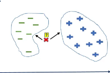
The k-nearest neighbor classifier is one of the distance-based learnings that classifies a data record based on the k most similar data (neighbors) in the training data set. The distance metric can be Euclidean distance for continues values and Hamming distance for discrete values. Although, the nearest neighbor classifier is one of the simplest machine learning algorithms, it requires a large computing power when calculating the distance of a data record to its neighbors. Also, this problem will be more challenging when the training data set is noisy [35]. In the example shown in Figure 2.4, the goal is to assign a class label to the unknown data record x based on the two existed classes.

(25)

11

2.5 Some applications for Interpretable models

Despite considering the predictive accuracy metrics as the main factor while evaluating models [4], there are other domains of applications in which the interpretability of the prediction is important for the users. For these applications, we should provide a model which is acceptable for the users like credit scoring [36], medicine [37] and bioinformatics [9]. This need becomes more serious when the model provides an unexpected prediction. In that case, the user asks good explanations from the system which highlights the crucial role of the interpretability of the model.

Medical domains, because of having critical context [38], require decision making to be always supported by explanations [37, 39] [40]. The necessity of explaining and justifying the decision when diagnosing a new patient is the main goal of Lavrac in her paper [41]. Also, she talks about the decision tree classifier which is easy to understand and can be used to support diagnosis without using the computer.

Bioinformatics is another application in which interpretability of models has an important role. The authors of [42] believe that the comprehensibility of discovered knowledge is required in bioinformatics because the discovered knowledge needs to be interpreted by biologist rather than accepting it blindly as a black-box. The paper introduces a data mining approach to generate a set of comprehensible rules by applying C4.5 algorithms which predict whether a protein has post-synaptic activity. According to their results, predicting the function of proteins based on their primary sequences is one of the challenges in bioinformatics due to the complex relationship between protein sequences and their functions. The rules were analyzed based on both their accuracy and

(26)

12

unexpectedness. The ones which are surprising could be more interesting for the biologist in determining novel insights.

Model comprehensibility and accuracy are also the key factors in building a successful credit scoring system. An expert in this field cannot trust a complex scorecard because of its low comprehensive explanation. Therefore, these black box predictive models cannot be very helpful in credit decision making. [1] investigates the performance of many classifiers in predicting and distinguishing between good and bad payers as represented in Figure 2.5 and 2.6 from [1] for German Credit dataset. Also, [43] discusses the difficulty of prediction in financial problems and tries to uncover the valuable patterns by applying Genetic Algorithms.

Figure 2. 5 unrestricted Bayesian network classifier learned using Markov Chain Monte for credit scoring in German credit dataset [1]

(27)

13

2.6 Prediction Errors Analysis

Analyzing and learning from errors in prediction, which are concerns in many works [6], mostly have been applied in detecting and predicting incorrect predictions in order to minimize its cost or in building a more accurate prediction model. Yet, less work directly focuses on how to explain the prediction errors. For this purpose, we need models which are able to explain the reasons behind the predictions.

One of the known examples in detecting misclassification is in spam classification when the classifier makes mistakes in distinguishing between spam and non-spam emails. In that case, we examine the instances in which the algorithm made errors on them to find out a systematic pattern to help us build new features and attributes to avoid these mistakes in the features. For example, usually, most of the spam emails are pharmacy emails or phishing ones. So, looking at them will help us to understand what features are useful to assign them correctly to a class [44].

(28)

14

Another work in analyzing the prediction errors is [45] which presents a general-purpose biologically plausible computational model, called SELP (Surprise → Explain → Learn → Predict). They use predictive coding which learns from only prediction errors and surprises in streaming data, unlike the traditional algorithms which continuously analyze all the data.

Applying interpretability of classifiers in explaining the classification process, especially for understanding the misclassification, is the goal of [46]. They design and implement a Visual Data Mining system for classifying remotely sensed images (VDM-RS). Their proposed system provides two views; one of them is the decision tree classifier which provides tracing and discovering of the classification steps and understanding how a sample has been classified correctly or even finding in which step it has been misclassified.

2.7 Automated decision making and discrimination

Nowadays, algorithmic systems for making decisions are widely used to facilitate decisions in a variety of fields such as medicine, banking, education or predictive policing [13]. However, these automated decisions can be very sensitive when applied to socially sensitive personal information such as demographics. The mining algorithms are trained from datasets which may be biased regarding a certain group such as women or minorities. Therefore, there is always a need to make sure that using data mining methods for socially sensitive decision making do not lead to discrimination and unfair treatment against a group of people due to their gender, age, religious or ethnicity [12].

(29)

15

Automated discrimination can happen as a direct result of data analytics. These unfair treatments can occur unintentionally; for instance, considering a neighborhood as a factor of ethnicity. For example, looking at demographic data related to the people who are living in certain area and frequently getting credit denial, we can find that they all related to the same ethnic minority [47]. Also, Lowry, in her paper [48], mentions another example regarding automatically discriminating decisions against female and minority applicants of St. George’s Hospital Medical School in the 1980s.

The discovery and prevention of automated discrimination has been moderately discussed in the literature [49] [14, 50-52].

2.8 Credit risk prediction

Repayment of the loan and interest is very important for the lending institutions because late or incomplete paying off the borrowed money will reduce their profits and will affect their services for new customers. When a bank receives a loan application, based on the applicant’s profile, the bank should decide whether or not to grant a loan to a customer. In this regard, there are two types of risks associated with the bank’s decision [53]:

1. Not approving the loan to a good credit risk customer, who is more likely to pay off the loan, leads to loss of business to the bank.

2. Approving the loan to a person with a bad credit risk, who is not able to repay the loan on time or in full amount, may harm the financial interests of the bank.

(30)

16

Therefore, financial institutions and banks are always investigating more accurate methods to analyze their customer’s credit information. Machine learning is one of the approaches in the field used for credit-risk evaluation by building an intelligent decision system to distinguish between good and bad payers based on the information provided for the applications.

An intelligence credit scoring system should be able to provide a clear insight to the experts about why and how an applicant has been chosen as good or bad [36]. One way that a bank can provide experts and customers a meaningful information about the logic for this algorithmic decision system and the consequences of such processing is applying a decision tree classifier. The graphical representation provided by this classifier makes it easy to follow the logic of decisions for the users, particularly the rejected applicants.

(31)

17 CHAPTER 3 METHODOLOGY

3.1 Introduction

This chapter will describe a methodology to help investigate reasons for incorrect predictions. In Phase 1, we will build a predictive model to find possible stereotypes learned by the decision tree classifier. Then, Phase 2, will detect the incorrect stereotypical predictions and the possible reasons behind them.

3.2 Discussion

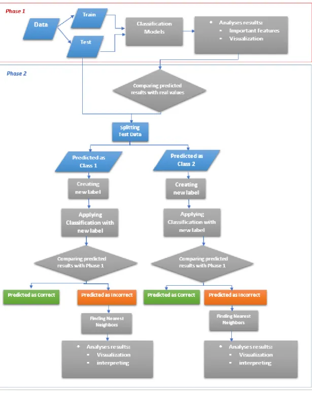
Our work is divided in two phases, Phase 1 and Phase 2. In Phase 1, we build our classification model by applying a decision tree classifier on the entire training data set to obtain the initial prediction results and the important features. We divide our dataset into training and testing with splitting ratio of 0.7 for training and 0.3 for testing.

Then, in Phase 2, based on the predicted results, we create a new training data set from the testing data in Phase 1, called “Predicted as Class 1” which consists of only records that have been predicted as “Class 1”. In the same way, we extract another training data subset for those that has been predicted as “Class 2” with the class name “Predicted as Class 2”. New labels are then assigned by comparing prediction results from Phase 1 with the true class labels. If the prediction and true class label are the same, the new label will be “correct”. Otherwise, we will assign the new label, “incorrect”. In

(32)

18

Phase 2, we learn a decision tree classifier again on the newly labeled subset, separately. Hence, by following the paths within the decision trees from both phases, for the records that have been labeled incorrectly in Phase 1 (with new label “incorrect” in Phase 2) and have the same predicted label (“incorrect”) in Phase 2, we try to determine which attribute is responsible for the incorrect prediction.

In each phase, we determine the optimal depth of decision trees and the minimum number of misclassified data records before learning our predictive model. Finding the optimal depth will avoid the overfitting and hence, considering irrelevant attributes in making decisions.

We continue our investigations by finding similar data records to the misclassified ones, among neighbors with the same and different actual class labels by using k nearest neighbors. Exploring shared characteristics promises to help find which features are the red flags and need to be considered when making decisions.

Moreover, the “important features” provided by the decision tree classifier are extracted to explore the possible key roles they may have in describing incorrect predictions.

In the next chapter, we present our experimental results which illustrate, in detail, how we apply this methodology to two real datasets.

(33)

19

(34)

20 CHAPTER 4 EXPERIMENTS

4.1 Introduction

In this chapter, we apply the methodology presented in Chapter 3 to two real datasets, Student Alcohol Consumption and German Credit, to explore the predictive rules after learning the decision tree classifier and describe which attributes can explain the incorrect predictions.

4.2 Discussion 4.2.1 Case study 1

Research showed that there are high rates of using alcohol among college students and young adults. These students are more likely to experience school problems such has higher absences and failing courses, legal problems such as arrests for drinking and driving, abuse of other drugs, etc. In our work, we use a real student alcohol consumption dataset to find out what are the potential attributes in categorizing addicted students from others.

4.2.1.1 Student Alcohol Consumption dataset

4.2.1.1.1 Phase 1

The Student Alcohol Consumption dataset is provided by Fabio Pagnotta, Hossain Mohammad Amran in UCI Machine Learning Repository [54] and it related to their research about finding the correlation between alcohol usage and the

(35)

socio-21

demographics, study time, and other behavioral attributes for Portuguese secondary school’s students in two datasets, student-mat.csv (students who have Math course) and student-por.csv (students who have Portuguese language course). In our thesis, we only use the Math course. This data set consists of 395 instances with 32 attributes with no missing values. Tables 4.1 and 4.2 provide more details about the attributes and their definitions.

Table 4. 1 Summary of the Student Alcohol Consumption Data Set information[55] Instances Attributes Missing values

Data 395 32 0

Table 4. 2 Student Alcohol Consumption Data Set’s Attribute Definition

Nr. Attributes Definition

1 school student's school (binary: "GP" - Gabriel Pereira or "MS" - Mousinho da Silveira)

2 sex student's sex (binary: "F" - female or "M" - male) 3 age student's age (numeric: from 15 to 22)

4 address student's home address type (binary: "U" - urban or "R" - rural)

5 famsize family size (binary: "LE3" - less or equal to 3 or "GT3" - greater than 3) 6 Pstatus parent's cohabitation status (binary: "T" - living together or "A" - apart) 7 Medu mother's education (numeric: 0 - none, 1 - primary education (4th grade), 2 –

5th to 9th grade, 3 – secondary education or 4 – higher education)

8 Fedu father's education (numeric: 0 - none, 1 - primary education (4th grade), 2 – 5th to 9th grade, 3 – secondary education or 4 – higher education)

9 Mjob mother's job (nominal: "teacher", "health" care related, civil "services" (e.g. administrative or police), "at_home" or "other")

10 Fjob father's job (nominal: "teacher", "health" care related, civil "services" (e.g. administrative or police), "at_home" or "other")

11 reason reason to choose this school (nominal: close to "home", school "reputation", "course" preference or "other")

12 guardian student's guardian (nominal: "mother", "father" or "other")

13 traveltime home to school travel time (numeric: 1 - <15 min., 2 - 15 to 30 min., 3 - 30 min. to 1 hour, or 4 - >1 hour)

14 studytime weekly study time (numeric: 1 - <2 hours, 2 - 2 to 5 hours, 3 - 5 to 10 hours, or 4 - >10 hours)

15 failures number of past class failures (numeric: n if 1<=n<3, else 4) 16 schoolsup extra educational support (binary: yes or no)

17 famsup family educational support (binary: yes or no)

18 paid extra paid classes within the course subject (Math or Portuguese) (binary: yes or no)

(36)

22

20 nursery attended nursery school (binary: yes or no) 21 higher wants to take higher education (binary: yes or no) 22 internet Internet access at home (binary: yes or no) 23 romantic with a romantic relationship (binary: yes or no)

24 famre quality of family relationships (numeric: from 1 - very bad to 5 - excellent) 25 freetime free time after school (numeric: from 1 - very low to 5 - very high)

26 goout going out with friends (numeric: from 1 - very low to 5 - very high)

27 Dalc workday alcohol consumption (numeric: from 1 - very low to 5 - very high) 28 Walc weekend alcohol consumption (numeric: from 1 - very low to 5 - very high) 29 health current health status (numeric: from 1 - very bad to 5 - very good)

30 absences number of school absences (numeric: from 0 to 93) 31 G1 first period grade (numeric: from 0 to 20)

32 G2 second period grade (numeric: from 0 to 20) 33 G3 final grade (numeric: from 0 to 20, output target)

34 Alc Alcohol consumption between week (numeric: from 1 - very low to 5 - very high)

Following [55] which is related to this dataset, we create a new attribute “Alc” which is a combination of two attributes “Walc,” weekend alcohol consumption, and “Dal,” workday alcohol consumption.

𝑨𝒍𝒄 = (𝑾𝒂𝒍𝒄 ∗ 𝟐 + 𝑫𝒂𝒍𝒄 ∗ 𝟓)/𝟕 (4.1)

After rounding the value, the result will be an integer between 1 and 5. Hence, we create a new attribute (new_target) which categorizes students to “Nondrinker” if “Alc” is less than 3 (1 and 2) and “drinker” if “Alc” equals 3, 4 or 5. Then in preprocessing, we convert “Nondrinker” to 0 and “drinker” to 1.

The next step is to divide our dataset into training and testing with splitting ratio of 0.7 for training and 0.3 for testing.

Before starting the classification, we try to find the optimal depth of the decision tree classifier which has the minimum number of incorrect predictions. It will help prevent overfitting: when the accuracy of the decision tree on the training data set is

(37)

23

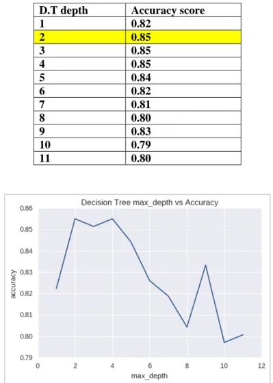
higher than the testing data. To find efficient parameters, we use “GridSearchCv” provided by “scikit-learn” which exhaustively considers all possible combinations of parameter values and chooses the best ones. According to the Table 4.3 and 4.4, we decide to choose the Max_depth=2 which has the best accuracy and the minimum number misclassified records.

Table 4. 3 Phase 1’s D.T. Classifier, Finding the Optimal Depth and Best Accuracy Score D.T depth Accuracy score

1 0.82 2 0.85 3 0.85 4 0.85 5 0.84 6 0.82 7 0.81 8 0.80 9 0.83 10 0.79 11 0.80

(38)

24

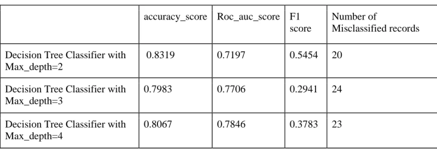
Table 4. 4 Phase 1’s D.T. Classifier, Comparing Classification Results with different Depths accuracy_score Roc_auc_score F1

score

Number of

Misclassified records Decision Tree Classifier with

Max_depth=2

0.8319 0.7197 0.5454 20

Decision Tree Classifier with Max_depth=3

0.7983 0.7706 0.2941 24

0.8067 0.7846 0.3783 23

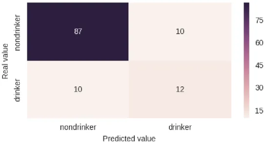
Now we fit the D.T. classifier with max_depth= 2 to the training and testing data sets with splitting ratio of 0.7 for training and 0.3 for testing to predict whether a student is a drinker or not. The classification results are shown in Table 4.5. According to the confusion matrix shown in Figure 4.2, we have 20 misclassified data records: 10 “drinker” students which has been predicted as “nondrinker” and 10 “nondrinker” students that has been predicted to “drinker”.

Table 4. 5 Phase 1’s D.T. Classifier’s Classification results with Max_depth=2 accuracy_score Roc_auc_score F1

score D.T. Classifier with

Max_depth=2

(39)

25

Figure 4. 2 Phase 1’s D.T. Classifier’s confusion matrix with max_depth=2

Also, the “important features” provided by decision tree classifier with max_depth=2 are “goout”, “sex” and “absences” that have greater effects on predictions. (Table 4.6)

Table 4. 6 Phase 1’s D.T. Classifier’s Important Features

features Degree of importance

goout 0.5566

sex_F 0.3923

absences 0.0510

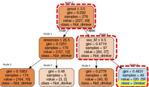
As it mentioned before, the decision tree’s graphical structure and if-then rules make it easy for general users to understand the prediction results. For example, in Figure 4.3 by following the path includes node 0, node 4, and then node 6, the user will find that if a student goes out frequently with friends and is a male, he is more likely to be a “drinker”, which is expected and does make sense.

(40)

26

Figure 4. 3 Phase 1’s D.T. diagram with Max_depth=2

(41)

27

Learning Decision Tree on Testing Data (unseen data) to find the paths:

After fitting the Decision Tree Classifier to the training dataset, we can use the decision_path() function from scikit-learn to find the nodes that were reached by each record in our testing dataset on the path from the root to leaf. This method converts testing data set which has 119 rows to a matrix of 119* 7, where 7 is the total number of nodes in the classifier model. By following the path for each specific record, we can find the attributes which caused the classifier to predict a class label incorrectly.

Table 4. 8 Number of misclassified data for testing data set in Phase 1 Number of misclassified data in Phase 1 20

Number of misclassified data ending in “Node 2” 8 Number of misclassified data ending in “Node 6” 10 Number of misclassified data ending in “Node 5” 2

Table 4. 9 Number of test records that go through each node * in the model Node * indicates a leaf node Number of records that passes through each node in testing data Number of Misclassified records from True Class “drinker”, which ends in node 2 Number of Misclassified records from True Class “drinker”, which ends in node 6 Number of Misclassified records from True Class “not drinker”, which ends in node 5 Path from Phase 1 (See Table 4.10 for each path) Index of Misclassified records 0 119 1 77 2* 77 8 0,1,2 '369','384','228','392','393, '41’,'249','89' 3* 0 4 42 5* 22 2 0,4,5 ‘318’, ‘61’ 6* 20 10 0,4,6 '304’,'161','172','354','6','307', '277', '242','351', '347' * refers to the decision nodes (leaves) in Figure 4.3.

(42)

28

Analyzing and Visualizing misclassified records in Decision Tree Classifier from Phase 1:

To learn more about the misclassified data records, we extract and display them in Tables 4.11-13. According to Table 4.9, we have eight misclassified data records that follow the Path 0, 1, 2 which indicates that students who do not go out frequently with friends and do not have many absences in their courses, are more likely to be nondrinkers. Among them, three students are with actual class label “drinker” and five students are with actual class label “nondrinker” (Table 4.10). To have a better visualization, we only show some of important attributes in this part.

Table 4. 10 Phase 1’s D.T. Classifier’s paths and rules that lead to misclassification

Phase 1, Decision Tree Classifier Path

Rule that causes misclassification

Number of test data records that were misclassified by this rule

Number of test data records that were

classified correctly by this rule Path 0, 1, 2 if ( goout <= 3.5 ) { if ( absences <= 26.5 ) { return nondrinker 8 69 Path 0,4,5 if ( goout > 3.5 ) { if ( sex_M <= 0.5 ) { return nondrinker 2 18 Path 0, 4, 6 if ( goout > 3.5 ) { if ( sex_M > 0.5 ) { return drinker 10 12

(43)

29

Table 4. 11 Misclassified records which end at node 2 (“goout” <= 3.5 and “absences” <= 26.5)

Table 4. 12 Misclassified records which end at node 5(“goout” > 3.5 and “sex_M” <= 0.5)

Column1 sex age Medu Fedu Mjob Fjob guardian traveltime studytime failures activities nursery freetime goout absences G1 G2 G3 Alc

Nondrinker F 17 3 4 at_home services father 1 3 0 yes no 3 4 0 11 11 10 3

Drinker F 16 1 1 services services father 4 1 0 yes no 5 5 6 10 8 11 5

Nondrinker sex age Medu Fedu Mjob Fjob guardian traveltime studytime failures activities nursery freetime goout absences G1 G2 G3 Alc

F 18 4 4 other teacher father 3 2 0 no no 2 2 10 14 12 11 3

M 21 1 1 other other other 1 1 3 no no 5 3 3 10 8 7 3

M 18 3 2 services other mother 3 1 0 no no 4 1 0 11 12 10 3

M 15 4 4 teacher other other 1 1 0 no no 4 3 8 12 12 12 3

M 16 0 2 other other mother 1 1 0 no no 3 2 0 13 15 15 3

Drinker sex age Medu Fedu Mjob Fjob guardian traveltime studytime failures activities nursery freetime goout absences G1 G2 G3 Alc

M 18 4 2 other other father 2 1 1 no yes 4 3 14 6 5 5 4

M 18 2 1 at_home other mother 4 2 0 yes yes 3 2 14 10 8 9 4

(44)

30

Nonrinker sex age Medu Fedu Mjob Fjob guardian traveltime studytime failures activities nursery freetime goout absences G1 G2 G3 Alc

M 19 3 3 other other other 1 2 1 yes yes 4 4 20 15 14 13 1

M 15 3 2 other other mother 2 2 2 no yes 4 4 6 5 9 7 2

M 17 4 4 teacher other mother 1 2 0 yes yes 4 4 0 13 11 10 2

M 17 4 3 services other mother 2 2 0 yes no 5 5 4 13 11 11 2

M 16 2 2 other other mother 1 2 0 no yes 4 4 0 12 12 11 1

M 19 4 4 teacher services other 2 1 1 no yes 3 4 38 8 9 8 1

M 18 4 4 teacher services mother 2 1 0 yes yes 2 4 22 9 9 9 2

M 17 3 3 health other mother 2 2 0 no yes 5 4 2 13 13 13 2

M 16 4 3 teacher other mother 1 1 0 yes no 4 5 0 6 0 0 1

M 18 4 3 teacher other mother 1 3 0 no yes 4 5 0 10 10 9 2

(45)

31 4.2.1.1.2 Phase 2

In this Phase, we split the test data set from Phase 1 into two subsets, “Predicted as a drinker”, for which the decision tree classifier from Phase 1 has predicted them as “drinker” and “Predicted as a nondrinker” for those that have been predicted as “nondrinker” by the decision tree classifier from Phase 1. Then for each subset, we create a new class label by comparing the predicted labels with the true labels. So, for the data set “Predicted as a drinker”, the new label (“new_target”) is “correct” if the real target (before applying the decision tree classifier) is “drinker” and the predicted value (after applying the decision tree classifier) is still a “drinker”. Otherwise, it should be “incorrect.” Similarly, for the subset “Predicted as a nondrinker”, if the person is really a “nondrinker” and the classifier has predicted them as a “nondrinker”, the new label is “correct”; otherwise, the new label is “incorrect”.

Table 4. 14 Phase 1’s Prediction results for Testing data set

Data Instances Attributes

Test Dataset from Phase 1 119 58

Records Predicted as drinker 22 58

Records Predicted as nondrinker 97 58

Table 4. 15 Phase 1’s Prediction results as “drinker” for Testing data set

Test data Predicted as drinker 22 58

Records Predicted as drinker correctly 12 58

Records Predicted as drinker incorrectly 10 58

Table 4. 16 Phase 1’s Prediction results as “nondrinker” for Testing data set

Test data Predicted as nondrinker 97 58

Records Predicted as nondrinker correctly 87 58

(46)

32

Building the D.T. Classifier for the subset of data that was predicted as “nondrinker”:

After Splitting the subset of data that was predicted as “nondrinker”, as shown in Table 4.17, we apply “GridSearchCv” to find the optimal depth for D.T. and the minimum number of misclassified records. According to Table 4.18, the confusion matrix report for both max_depth= 1 and max_depth=2 are the same. Therefore, to have a better and deeper view of the decision tree classifier, we decide to choose max_depth=2 to continue working.

Table 4. 17 Splitting the Subset of data that was Predicted as “nondrinker” to training and testing data set

Instances Attributes Missing values

Predicted as nondrinker 97 58 0

Training Data_3 (70% from row 1) 67 58 0

Testing Data_3 (30% from row 1) 30 58 0

Table 4. 18 Phase 2’s D.T. Classifier, Finding the Optimal Depth and Best Accuracy Score for the subset of data that was predicted as “nondrinker” in Phase 1

D.T. depth Accuracy score

1 0.8656 2 0.8656 3 0.8507 4 0.8507 5 0.8507 1 0.8656

(47)

33

Figure 4. 4 Phase 2’s D.T. Classifier, Finding the Optimal Depth and Best Accuracy Score for

the subset that was predicted as “nondrinker” in Phase 1

Table 4. 19 Phase 2’s D.T. Classifier, Comparing Classification Results with different Depths

for the subset that was predicted as “nondrinker” in Phase 1 accuracy_score Roc_Auc_score F1

score

Number of Misclassified records Decision Tree Classifier with

Max_depth=1

0.9 0.625 0.4 3

0.9 0.552 0.4 3

0.866 0.552 0.333 4

Learning the D.T. on Training Data_3 (the training data of the subset that was predicted as “nondrinker”) and then the prediction results are shown in Figure 4.5 as a confusion matrix. Indeed, Phase 2 predicts if Phase 1’s prediction is incorrect. The data records for which their real value was “incorrect” in Phase 1 and they have been predicted to “incorrect” in Phase 2 can help us to find the rules that lead to incorrect predictions (incorrect stereotypical predictions). Here there is only one instance with this condition and we call it record “A” (Figure 4.5). For further exploration, we will go through the paths that led to predictions in Phase 1 and Phase 2 for data record “A”.

(48)

34

Figure 4. 5 Phase 2’s D.T. Classifier, Confusion_matrix with max_depth=2 for the subset of data that was predicted as “nondrinker” in Phase 1

Phase 2’s D.T. Classifier’s Important features for the subset of data that was predicted as “nondrinker” in Phase 1 with max_depth= 2:

Here the decision dree classifier chooses attributes “traveltime” and “Fedu” (Father education) as the important ones in making predictions. These features may hold the key to explaining and fixing incorrectly classified stereotyped data records. (Table 4.20)

Table 4. 20 Phase 2’s D.T. Classifier’s Important features for the subset of data that was

predicted as “nondrinker” in Phase 1 with max_depth= 2

Features Degree of importance

traveltime 0.5179

Fedu 0.4820

Fjob_health 0.0000

Medu 0.0000

absences 0.0000

Decision tree extracted rules for data predicted as “nondrinker” in Phase 1, with max_depth=2:

Table 4.21 and Figure 4.6 display the graphical prediction results and decision rules generated be the decision tree classifier for this subset of data.

(49)

35

Table 4. 21 Phase 2’s D.T. Classifier’s rules with Max_depth=2 for the subset of data that was predicted as “nondrinker” in Phase 1

Decision Tree diagram for the subset of data was predicted as “nondrinker” in Phase 1, with max_depth=2:

Figure 4. 6 Phase 2’s D.T. diagram with Max_depth=2 for the subset of data that was predicted

as “nondrinker” in Phase 1

Analyzing and Visualizing the records that have label “incorrect” in Phase 2 and have been predicted as “incorrect” by the Phase 2 Decision Tree Classifier:

(50)

36

Table 4. 22 The record of data that predicted as “nondrinker” with class label “incorrect” from Phase 1, which has been predicted to class label “incorrect” in Phase 2

Drinker sex age Medu Fedu Mjob Fjob guardian traveltime studytime failures activities nursery freetime goout absences G1 G2 G3 Alc

(51)

37

Table 4. 23 Phase 2’s D.T. Classifier’s paths and rules that lead to misclassification for the

subset of data that was predicted as “nondrinker” in Phase 1

Rules that lead to misclassification

Number of test data records misclassified by this rule Number of test data records classified correctly by this rule Path 0, 1, 2 if ( traveltime <= 3.5 ) { if ( Fedu <= 3.5 ) { return correct 2 22 Path 0,4 if ( traveltime > 3.5 ) return incorrect 1 0

Building a Phase 2’s D.T Classifier for the subset of data that was predicted as “drinker” by D.T from Phase 1 :

Table 4. 24 Splitting the Subset of data that was Predicted as “drinker” to training and testing data set

Instances Attributes Missing values

Predicted as drinker 22 58 0

Training Data_4 (70% from row 1) 15 58 0

Testing Data_4 (30% from row 1) 7 58 0

Finding the optimal Depth for the subset of data that was predicted as “drinker” in Phase 1:

According to Table 4.25 which shows the results of searching the best accuracy score and minimum number of misclassified data records by applying “GridSearchCv” to Training Data_4, both max_depth= 1 and max_depth=2 generate the same accuracy scores. So, to have a better and deeper view of decision tree classifier we decide to choose max_depth=2 to continue working.

(52)

38

Table 4. 25 Phase 2’s D.T. Classifier, Finding the Optimal Depth and Best Accuracy Score for the subset of data that was predicted as “drinker” in Phase 1

D.T depth Accuracy score

1 0.4666

2 0.4666

3 0.4666

4 0.4000

5 0.4000

Comparing Classification results with different depth of tree Phase2:

Table 4. 26 Phase 2’s D.T. Classifier, Comparing Classification Results with different Depths

for the subset of data that was predicted as “drinker” in Phase 1 accuracy_score Roc_auc_score F1 score Number of Misclassified records Decision Tree Classifier with Max_depth=1 0.4285 0.45 0.5 4 Decision Tree Classifier with Max_depth=2 0.5714 0.7 0.5714 3 Decision Tree Classifier with Max_depth=3 0.5714 0.7 0.5714 3

Figure 4. 7 Phase 2’s D.T. Classifier, Finding the Optimal Depth and Best Accuracy Score for the subset of data that was predicted as “drinker” in Phase 1

(53)

39

Phase 2’s D.T Confusion_matrix with max_depth=2 for data predicted as “drinker” in Phase 1:

Figure 4. 8 Phase 2’s D.T. Classifier’s Confusion matrix with max_depth=2 for the subset of data that was predicted as “drinker” in Phase 1

Phase 2’s Decision Tree Classifier’s Important features for data predicted as “drinker” during Phase 1:

Table 4. 27 Phase 2’s D.T. Classifier’s Important features for the subset of data that was predicted as “drinker” in Phase 1 with max depth= 2

features Degree of importance

G2 0.4000

Medu 0.3333

G1 0.2666

Fjob_other 0.0000

absences 0.0000

These important features may hold the key to understanding the basis for the incorrect stereotypical predictions from Phase 1.

Extracting rules for Phase 2’s Decision Tree Classifier trained on data predicted as “drinker” in Phase 1:

(54)

40

Table 4. 28 Phase 2’s D.T. Classifier’s rules with Max_depth=2 for the subset of data that was predicted as “drinker” in Phase 1

Phase 2’s Tree Diagram for Decision Tree Classifier for data that was predicted as “drinker” during Phase 1:

Figure 4. 9 Phase 2’s D.T. diagram with max depth=2 for the subset of data that was predicted

as “drinker” in Phase 1

In this step, according to the confusion matrix, we have two records for which their real value was “incorrect” and they have been predicted to “incorrect” (Figure 4.8).

if ( Medu <= 3.5 ) { if ( G1 <= 5.5 ) {

return incorrect ( 1 examples ) }

else {

return correct ( 8 examples ) }

} else {

if ( G2 <= 11.5 ) {

return incorrect ( 4 examples ) }

else {

return correct ( 2 examples ) }

(55)

41

We will visualize these examples in Table 4.29. These two records have been predicted as a drinker in Phase 1 because their “goout” is greater than 3.5 and they are males ( sex_M > 0.5). Then in Phase 2, because of having “Medu” > 3.5 and G2 <= 11.5, the model predicts them as a label of “incorrect”.

(56)

42

Table 4. 29 The records of data that predicted as “drinker” with class label “incorrect” from Phase 1, which has been predicted to class label “incorrect” in Phase 2.

Nondrinker sex age Medu Fedu Mjob Fjob guardian traveltime studytime failures activities nursery freetime goout absences G1 G2 G3 Alc

M 18 4 4 teacher services mother 2 1 0 yes yes 2 4 22 9 9 9 2

(57)

43 4.2.1.1.3 Analyzing the results

Table 4.30 shows student “A” among her neighbors who all traverse the same path in Phase1’s D.T because they go out a lot with friends and are females and, like A, have been predicted to be “nondrinker”. The only difference is their real label: A was really a “drinker” but A1, A2 and A3 were really “nondrinkers”. Looking at their similarity in going through the same path in Phase 1, we can understand how our model has learned to predict A, like A1, A2 and A3, as a “nondrinker”. Their different decision tree paths in Phase 2 indicate how A is suspected to be a “drinker” in reality. As Table 4.30 shows, she spends a long time (more than 1 hour) getting home from school. This time may be spent with peers without parent supervision and possibly lead to drinking more alcohol.

The next table, Table 4.31, displays information related to record A and her neighbors who are all drinkers in reality but have been predicted incorrectly as “nondrinker”. In Phase 1, their D.T paths followed two rules which caused the prediction “nondrinker”; one path says, if a student goes out frequently with friends but is a female, she is more likely to be a “nondrinker,” and another one says having not too much hanging out with friends and not many absences in classes, counts for being a “nondrinker”. Both rules make sense and are expected.

Record A and A’3 both have been predicted incorrectly as “nondrinkers” and our model in Phase 2 succeed to detect this wrong prediction. Their path in Phase 2 tells us which attributes may have misled the model in Phase 1, namely, having high “traveltime” to get back home from school, for both students, as shown in Table 4.31.