arxiv: v4 [math.dg] 29 Jul 2014

(1)

arXiv:1306.5318v4 [math.DG] 29 Jul 2014

The curvature: a variational approach

A. Agrachev

D. Barilari

L. Rizzi

SISSA, Trieste, Italy and Steklov Mathematical Institute, Moscow, Russia. E-mail address: [email protected]

CNRS, CMAP École Polytechnique and Équipe INRIA GECO Saclay Île-de-France, Paris, France.

Current address: Université Paris Diderot - Paris 7, Institut de Mathematique de Jussieu, UMR CNRS 7586 - UFR de Mathématiques.

E-mail address: [email protected] SISSA, Trieste, Italy.

Current address: CNRS, CMAP École Polytechnique and Équipe INRIA GECO Saclay Île-de-France, Paris, France.

(2)

2010Mathematics Subject Classification. Primary: 49-02, 53C17, 49J15, 58B20

Key words and phrases. sub-Riemannian geometry, affine control systems, curvature, Jacobi curves

The first author has been supported by the grant of the Russian Federation for the state support of research, Agreement No 14 B25 31 0029. The second author has been supported by the European Research Council, ERC StG 2009 “GeCoMethods”, contract number 239748, by the ANR Project GCM, program “Blanche”, project number NT09-504490. The third author has been supported by INdAM (GDRE CONEDP) and Institut Henri Poincaré, Paris, where part of this research has been carried out. We warmly thank Richard Montgomery and Ludovic Rifford for their careful reading of the

manuscript. We are also grateful to Igor Zelenko and Paul W.Y. Lee for very stimulating discussions. Abstract. The curvature discussed in this paper is a rather far going generalisation of the Riemann-ian sectional curvature. We define it for a wide class of optimal control problems: a unified framework including geometric structures such as Riemannian, sub-Riemannian, Finsler and sub-Finsler struc-tures; a special attention is paid to the sub-Riemannian (or Carnot–Carathéodory) metric spaces. Our construction of curvature is direct and naive, and it is similar to the original approach of Riemann. Surprisingly, it works in a very general setting and, in particular, forallsub-Riemannian spaces.

(3)

Introduction

The curvature discussed in this paper is a rather far going generalization of the Riemannian sectional curvature. We define it for a wide class of optimal control problems: a unified framework including geometric structures such as Riemannian, sub-Riemannian, Finsler and sub-Finsler structures; a special attention is paid to the sub-Riemannian (or Carnot–Carathéodory) metric spaces. Our construction of the curvature is direct and naive, and it is similar to the original approach of Riemann. Surprisingly, it works in a very general setting and, in particular, forall sub-Riemannian spaces.

Interesting metric spaces often appear as limits of families of Riemannian metrics. We first try to explain the nature of our curvature by describing the case of a contact sub-Riemannian structure in terms of such a family and then we move to the general construction.

Let M be an odd-dimensional Riemannian manifold endowed with a contact vector distribution D _⊂ _{T M}_{. Given} _x₀_{, x}₁ _∈ _M_{, the contact sub-Riemannian distance} d(_x₀_{, x}1) is the infimum of the

lengths of Legendrian curves connecting x0 and x1. Recall that Legendrian curves are just integral curves of the distribution D. The metric d is easily realized as the limit of a family of Riemannian

metricsdεas_ε_→0. To definedε we start from the original Riemannian structure on_M, keep fixed the

length of vectors fromD and multiply by 1

ε the length of the orthogonal toD tangent vectors toM. It

is easy to see thatdε_→_d_{uniformly on compacts in}_M_×_M _as _ε_→_0.

The distance converges, what about the curvature? Letωbe a contact differential form that

annihi-latesD, i.e. D=_ω⊥. Given_v₁_{, v}₂_∈_T_x_{M, v}₁_∧_v₂₆= 0_,we denote by_Kε₍_v

1∧v2) the sectional curvature for the metricdε and section span_{_v₁_{, v}₂_}. It is not hard to show that_Kε(_v₁_∧_v2)_{→ −∞}if_v₁_{, v}₂_∈D anddω(v1, v2)6= 0. Moreover, Ricε(v)→ −∞as ε→0 for any nonzero vectorv∈D, where Ricεis the Ricci curvature for the metricdε. On the other hand, the distance between_xand the conjugate locus of

xtends to 0 asε_→0 andKε₍_v

1∧v2) tends to +∞for some v1, v2∈TxM, as well as Ricε(v) for some

v_∈TxM.

What about the geodesics? For any ε > 0 and any v _∈ TxM there is a unique geodesic of the

Riemannian metricdεthat starts from_xwith velocity_v. On the other hand, the velocities of all geodesics

of the limit metricdbelong toD_{and for any nonzero vector}_v_∈D_{there exists a one-parametric family} of geodesics whose initial velocity is equal to v. Too bad up to now, and here is the first encouraging

fact: the family of geodesic flows converges if we re-write it as a family of flows on the cotangent bundle. Indeed, any Riemannian structure on M induces a self-adjoint isomorphism G : T M → T∗M,

where _hGv, vi is the square of the length of the vectorv ∈T M, andh·,·i denotes the standard pairing between tangent and cotangent vectors. The geodesic flow, treated as flow on T∗M is a Hamiltonian

flow associated with the Hamiltonian functionH :T∗_M _→_R_{, where}_H₍_λ_{) =} 1

2hλ, G−1λi, λ∈T∗M. Let (λ(t), γ(t)) be a trajectory of the Hamiltonian flow, withλ(t)_∈T∗

γ(t)M. The square of the Riemannian distance fromx0is a smooth function on a neighbourhood ofx0inM and the differential of this function at γ(t) is equal to 2tλ(t) for any smallt ≥0. LetHε _{be the Hamiltonian corresponding to the metric} dε_{. It is easy to see that} _Hε _{converges with all derivatives to a Hamiltonian} _H0_{. Moreover, geodesics} of the limit sub-Riemannian metric are just projections toM of the trajectories of the Hamiltonian flow

onT∗_M _{associated to}_H0_.

We can recover the Riemannian curvature from the asymptotic expansion of the square of the distance fromx0 along a geodesic: this is essentially what Riemann did. Then we can write a similar expansion for the square of the limit sub-Riemannian distance to get an idea of the curvature in this case. Note that the metrics dεconverge tod with all derivatives in any point of_M _×_M, wheredis smooth. The

metrics dε are not smooth at the diagonal but their squares are smooth. The point is that no power of dis smooth at the diagonal! Nevertheless, the desired asymptotic expansion can be controlled.

Fix a point x0 ∈ M and λ0 ∈ Tx∗0M such that hλ0,Di 6= 0. Let (λ

ε₍_t₎_{, γ}ε₍_t_{)), for} _ε

≥ 0, be the trajectory of the Hamiltonian flow associated to the HamiltonianHε_{and initial condition (}_λ

(6)

set: cεt(x) . =₋1 2t(d ε₎2₍_{x, γ}ε₍_t_{)) if} _{ε >}₀_, _c0 t(x) . =₋1 2td 2₍_{x, γ}0₍_t₎₎_. There exists an interval (0, δ) such that the functionscε

t are smooth atx0for allt∈(0, δ) and allε≥0. Moreover,dx0c ε t=λ0. Let ˙cεt =∂t∂c ε t, thendx0c˙ ε

t= 0. In other words,x0is a critical point of the function ˙

cε

t and its Hessiand2x0c˙

ε

t is a well-defined quadratic form onTx0M. Recall thatε= 0 is available, but t must be positive. We are going to study the asymptotics of the family of quadratic formsd2

x0c˙

ε

t ast→0

for fixedε. This asymptotic is a little bit different forε >0 andε= 0. The change reflects the structural difference of the Riemannian and sub-Riemannian metrics and emphasises the role of the curvature. In this approach, the curvature is encoded in the function ˙ct(x). A geometrical interpretation of such a

function can be found in Appendix H.

Givenv, w_∈TxM, ε >0, we denotehv|wiε=hGεv, withe inner product generatingdε. Recall that

hv_|v_iεdoes not depend onεifv∈Dandhv|viε→ ∞(ε→0) ifv /∈D; we will write|v|2=. hv|viεin the

first case. For fixedε >0, we have: d2 x0c˙ ε t(v) = 1 t2hv|viε+ 1 3hRε( ˙γε, v) ˙γε)|viε+O(t), v∈Tx0M,

where ˙γε_{= ˙}_γε_{(0) and}_Rε _{is the Riemannian curvature tensor of the metric}_dε_{. For}_ε_{= 0, only vectors}

v∈D have a finite length and the above expansion is modified as follows:

d2 x0c˙ 0 t(v) = 1 t2Iγ(v) + 1 3Rγ(v) +O(t), v∈D∩Tx0M,

where _Iγ(v)≥ |v|2 andRγ is thesub-Riemannian curvature atx0 along the geodesicγ=γ0. BothIγ

and_Rγ are quadratic forms onDx0

.

=D_∩_T_x

0M. The principal “structural” termIγ has the following properties:

max_{Iγ(v)|v∈Dx0, |v| 2_{= 1}

}= 4,

Iγ(v) =|v|2 if and only ifdω(v,γ˙(0)) = 0.

In other words, the symmetric operator onD_x₀ associated with the quadratic form_I_γ has eigenvalue 1 of multiplicity dimD_x

0−1 and eigenvalue 4 of multiplicity 1. The trace of this operator, which, in this case, does not depend onγ, equals dimD_x

0+ 3. This trace has a simple geometric interpretation, it is equal to the geodesic dimension of the sub-Riemannian space.

The geodesic dimension is defined as follows. Let Ω_⊂M be a bounded and measurable subset of positive volume and let Ωx0,t, for 0 ≤t≤1, be a family of subsets obtained from Ω by the homothety of Ω with respect to a fixed pointx0along the shortest geodesics connectingx0 with the points of Ω, so that Ωx0,0={x0}, Ωx0,1= Ω. The volume of Ωx0,thas ordert

Nx0, whereN_x

0 is the geodesic dimension atx0 (see Section 5.6 for details).

Note that the topological dimension of our contact sub-Riemannian space is dimD_x

0 + 1 and the Hausdorff dimension is dimD_x

0+ 2. All three dimensions are obviously equal for Riemannian or Finsler manifolds. The structure of the term_Iγ and comparison of the asymptotic expansions ofd2x0c˙

ε

t forε >0

andε= 0 explains why sectional curvature goes to_−∞for certain sections.

The curvature operator which we define can be computed in terms of the symplectic invariants of the so-called Jacobi curve, namely a curve in the Lagrange Grassmannian related with the linearisation of the Hamiltonian flow. These symplectic invariants can be computed, in principle, via an algorithm which is, however, quite hard to implement. Explicit computations of the contact sub-Riemannian curvature will appear in a forthcoming paper. The current paper deals with the general setting. A precise construction in full generality is presented in the forthcoming sections but, since the paper is long, we find it worth to briefly describe the main ideas in the introduction.

LetM be a smooth manifold, D _⊂_{T M} be a vector distribution (not necessarily contact),_f₀ be a vector field onM andL:T M _→M be a Tonelli Lagrangian (i.e. L_T

xM has a superlinear growth and

its Hessian is positive definite for anyx∈M). Admissible pathsonM are curves whose velocities belong

to the “affine distribution”f0+D. LetAtbe the space of admissible paths defined on the segment [0, t]

andNt={(γ(0), γ(t)) :γ∈ At} ⊂M×M. The optimal cost (or action) functionSt:Nt→Ris defined

as follows: St(x, y) = inf Z t 0 L( ˙γ(τ))dτ :γ∈ At, γ(0) =x, γ(t) =y .

(7)

The space_At equipped with the W1,∞-topology is a smooth Banach manifold; the functionalJt:γ7→

Rt

0L( ˙γ(τ))dτ and the evaluation mapsFτ:γ7→γ(τ) are smooth onAt.

The optimal costSt(x, y) is the solution of the conditional minimum problem for the functionalJt

under conditionsF0(γ) =x, Ft(γ) =y. The Lagrange multipliers rule for this problem reads:

(1.1) dγJt=λtDγFt−λ0DγF0.

Hereλtandλ0 are “Lagrange multipliers”,λt∈Tγ∗(t)M, λ0∈Tγ∗(0)M. We have:

DγFt:TγAt→Tγ(t)M, λt:Tγ(t)M →R,

and the compositionλtDγFtis a linear functional onTγAt. Moreover, Eq. (1.1) implies that

(1.2) dγJτ =λτDγFτ−λ0DγF0,

for someλτ ∈T_γ∗₍_τ₎M and any τ ∈[0, t]. The curveτ 7→λτ is a trajectory of the Hamiltonian system

associated to the HamiltonianH :T∗_M _→_R_{defined by}

H(λ) = max

v∈f0(x)+D_x(hλ, vi −L(v)), λ∈T ∗

xM, x∈M.

Moreover, any trajectory of this Hamiltonian system satisfies relation (1.2), where γ is the projection of the trajectory to M. Trajectories of the Hamiltonian system are called normal extremals and their projections toM are callednormal extremal trajectories.

We recover the sub-Riemannian setting whenf0= 0,L(v) =1₂hGv, vi. In this case, the optimal cost is related with the sub-Riemannian distanceSt(x, y) = ₂1_td2(x, y), and normal extremal trajectories are

normal sub-Riemannian geodesics.

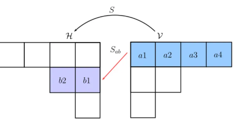
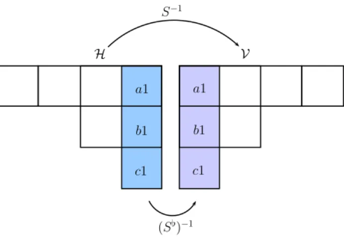
Let γ be an admissible path; the germ of γ at the point x0 =γ(0) defines a flag in Tx0M {0} = F_γ0 _⊂F_γ1 _⊂F_γ2 _⊂_{. . .} _⊂_T_x₀_M in the following way. Let _V be a section of the vector distribution D such that ˙γ(t) =f0(γ(t)) +V(γ(t)), t≥0,andP0,t be the local flow onM generated by the vector field

f0+V; thenγ(t) =P0,t(γ(0)). We set: Fi γ = span dj dtj t=0 (P0,t)−1_∗ Dγ(t):j= 0, . . . , i−1 . The flagFi

γ depends only on the germs off0+D andγat the initial pointx0. A normal extremal trajectory γ is called ample if Fm

γ = Tx0M for some m > 0. If γ is ample, thenJt(γ) =St(x0, γ(t)) for all sufficiently smallt >0 andSt is a smooth function in a neighbourhood

of (γ(0), γ(t)). Moreover, ∂St ∂y y=γ(t) = λt, ∂St ∂x

x=γ(0) =−λ0, where λt is the normal extremal whose projection isγ.

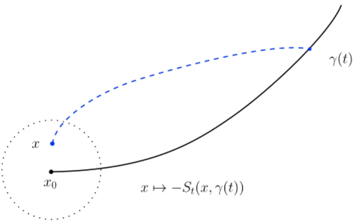
We setct(x)=. −St(x, γ(t)); thendx0ct=λ0 for anyt >0 andx0 is a critical point of the function ˙

ct. The Hessian of this functiond2x0c˙t is a well-defined quadratic form onTx0M. We are going to write an asymptotic expansion ofd2

x0c˙t

_D

x0

as t→0 (see Theorem A):

d2x0c˙t(v) = 1

t2Iγ(v) + 1

3Rγ(v) +O(t), ∀v∈Dx0.

Now we introduce a natural Euclidean structure onTx0M. Recall that L|Tx0M is a strictly convex function, andd2

w(L|Tx0M) is a positive definite quadratic form onTx0M, ∀w∈Tx0M. If we set |v| 2

γ =

d2 ˙

γ(0)(L|Tx0M)(v), v∈Tx0M we have the inequality

Iγ(v)≥ |v|γ2, ∀v∈Dx0.

The inequality _Iγ(v) ≥ |v|2γ means that the eigenvalues of the symmetric operator on Dx0 associated with the quadratic form_Iγ are greater or equal than 1. The quadratic formRγ is thecurvature of our

constrained variational problem along the extremal trajectoryγ.

A mild regularity assumption allows to explicitly compute the eigenvalues of _Iγ. We set γε(t) =

γ(ε+t) and assume that dimF_γi

ε = dimF

i

γ for all sufficiently small ε ≥ 0 and all i. Then di =

dimFi

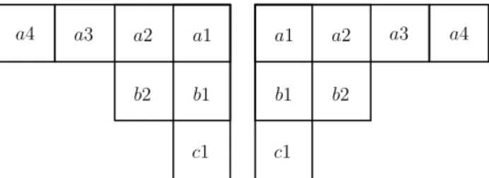
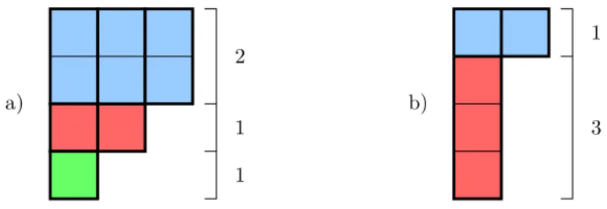
γ−dimFγi−1, for i≥1 is a non-increasing sequence of natural numbers withd1= dimDx0 =k. We draw a Young tableau with di blocks in thei-th column and we definen1, . . . , nk as the lengths of

(8)

its rows (that may depend onγ). n1 . . . n2 . . . dm .. . ... dm−1 nk−1 nk d2 d1

The eigenvalues of the symmetric operator_Iγ are n21, . . . , n2k (see Theorem B). Some of these numbers

may be equal (in the case of multiple eigenvalues) and are all equal to 1 in the Riemannian case. In the sub-Riemannian setting, the trace of_Iγ is

tr_Iγ=n21+· · ·+n2k= m

X

i=1

(2i₋1)di,

when computed for generic normal sub-Riemannian geodesic, is equal to the geodesic dimension of the space (see Theorem D).

The construction of the curvature presented here was preceded by a rather long research line (see [AL14,Agr08,AG97,AZ02,LZ11,ZL09]). For what concerns the alternative approaches to this topic,

in recent years, several efforts have been made to introduce a notion of curvature to non-Riemannian situations, such as sub-Riemannian manifolds and, more in general, metric measure spaces. Motivated by the lack of classical Riemannian tools (such as the Levi-Civita connection and the theory of Jacobi fields) different approaches have been explored in order to extend some classical results in geometric analysis to such structures. In particular, to this extent, different notions of generalized Ricci curvature bound have been introduced.

For instance, one can see [BG11,BW13] and references therein for a heat equation approach to the

generalization of the curvature-dimension inequality and [AGS14,LV09,Stu06a,Stu06b] and references

therein for an optimal transport approach to the generalization of Ricci curvature.

1.1. Structure of the paper

In Chapters 2–4 we give a detailed exposition of the main constructions in a more general and flexible setting than in this introduction. Chapter 5 is devoted to the specification to the case of sub-Riemannian spaces and to some further results: the proof that ample geodesics always exist (Theorem 5.17), an asymptotic expansion of the sub-Laplacian applied to the square of the distance (Theorem C), the computation of the geodesic dimension (Theorem D).

Before entering into details of the proofs, we end Chapter 5 by repeating our construction for one of the simplest sub-Riemannian structures: the Heisenberg group. In particular, we recover by a direct computation the results of Theorems A, B and C.

The proofs of the main results are concentrated in Chapters 6–8 where we introduce the main technical tools: Jacobi curves, their symplectic invariants and Li–Zelenko structural equations.

1.2. Statements of the main theorems

The main results, namely Theorems A, B, C and D, are spread in Part I of the paper. For convenience of the reader we collect them here, without any pretence at completeness. To be consistent with the original statements, in this section we express the dependence of the operators and the scalar product onγthrough the associated initial covectorλ.

Let γ : [0, T] _→ M be an ample geodesic with initial covector λ _∈ T∗

x0M, and let Qλ(t) be the symmetric operator associated with the second derivatived2

x0c˙tvia the scalar producth·|·iλ, defined for sufficiently smallt >0.

(9)

Theorem A (Section 4.4). The map t_7→t2

Qλ(t) can be extended to a smooth family of operators

onD_x

0 for smallt≥0, symmetric with respect toh·|·iλ. Moreover, Iλ= lim. t→0+t 2 Qλ(t)≥I>0, as operators on(D_x 0,h·|·iλ). Finally d dt t=0 t2_Qλ(t) = 0. Then, letλ_∈T∗

x0M be the initial covector associated with an ample geodesic. Thecurvatureis the symmetric operator_Rλ:Dx0 →Dx0 defined by

Rλ=. 3 2 d2 dt2 t=0 t2Qλ(t).

Moreover, the Ricci curvature at λ_∈ T∗

x0M is defined by Ric(λ)

.

= tr_Rλ. In particular, we have the

following Laurent expansion for the family of symmetric operators_Qλ(t) :Dx0 →Dx0

(_∗) _Qλ(t) =

1

t2Iλ+ 1

3Rλ+O(t), t >0.

Remark. Eq. (_∗) is crucial in our approach to curvature. As we will see, on a Riemannian manifold D_x

0 =Tx0M and h·|·iλ =h·|·iis the Riemannian scalar product for allλ∈T ∗

x0M. The specialisation of Eq. (_∗) leads to the following identities:

Iλ=I, Rλw=R∇(v, w)v, ∀w∈Tx0M,

where v= ˙γ(0) is the initial vector of the fixed geodesic dual to the initial covectorλ, whileR∇ is the Riemannian curvature tensor (see Section 4.5.1). The operator _Rλ is symmetric with respect to the

Riemannian scalar product and, seen as a quadratic form onTx0M, it computes the sectional curvature of the planes containing the direction of the geodesic.

Theorem B (Section 4.4.1). Let γ : [0, T]→ M be an ample and equiregular geodesic. Then the symmetric operator _Iλ:Dx0 →Dx0 satisfies

(i) spec_Iλ={n21, . . . , n2k},

(ii) tr_Iλ=n21+. . .+n2k.

Let M be a sub-Riemannian manifold and let ∆µ be the sub-Laplacian associated with a smooth

volumeµ. The next result is an explicit expression for the asymptotics of the sub-Laplacian of the squared distance from a geodesic, computed at the initial pointx0 of the geodesicγ. Let ft=. 1₂d2(·, γ(t)).

TheoremC (Section 5.4). Let γbe an equiregular geodesic with initial covectorλ_∈T∗

x0M. Assume

also thatdimD _{is constant in a neighbourhood of}_x₀_{. Then there exists a smooth}_n_-form_ω _{defined along}

γ, such that for any volume formµ onM,µγ(t)=eg(t)ωγ(t), we have ∆µft|x0 = trIλ−g˙(0)t−

1 3Ric(λ)t

2₊_O₍_t3₎_.

Let x0 ∈ M and let Σx0 ⊂ M be the set of points x such that there exists a unique minimizer

γ : [0,1] → M joining x0 with x, which is not abnormal and x is not conjugate to x0 along γ. A fundamental result (see [Agr09] or also Theorem 5.8) is that the set Σx0 is precisely the set of smooth points for the functionx_7→d2(_x₀_{, x}).

Let Ωx0,t be the homothety of a set Ω⊂Σx0 with respect to x0 along the geodesics connecting x0 with the points of Ω.

Theorem D (Section 5.6). Let µ be a smooth volume. For any bounded, measurable set Ω_⊂Σx0,

with0< µ(Ω)<+_∞we have

µ(Ωx0,t)∼t

Nx0, fort→0.

(10)

(11)

Part 1

(12)

(13)

CHAPTER 2

General setting

In this section we introduce a general framework that allows to treat smooth control system on a manifold in a coordinate free way, i.e. invariant under state and feedback transformations. For the sake of simplicity, we will restrict our definition to the case of nonlinear affine control systems, although the construction of this section can be extended to any smooth control system (see [Agr08]).

2.1. Affine control systems

Definition 2.1. LetM be a connected smoothn-dimensional manifold. Anaffine control system

onM is a pair (U_{, f}) where:

(i) Uis a smooth rank _kvector bundle with base _M and fiberU_x i.e., for every _x_∈_M, U_x is a

k-dimensional vector space,

(ii) f :U_→_{T M} is a smooth affine morphism of vector bundles, i.e. the diagram (2.1) is commu-tative andf isaffine on fibers.

(2.1) U πU ! ! ❈ ❈ ❈ ❈ ❈ ❈ ❈ ❈ f / /_{T M} π M

The mapsπU andπare the canonical projections of the vector bundlesUandT M, respectively.

We denote points inUas pairs (_{x, u}), where_x_∈_M and_u_∈U_xis an element of the fiber. According to this notation, the image of the point (x, u) throughf isf(x, u) orfu(x) and we prefer the second one

when we want to emphasizefu as a vector onTxM. Finally, letL∞([0, T],U) be the set of measurable,

essentially bounded functionsu: [0, T]_→U.

Definition 2.2. A Lipschitz curveγ: [0, T]_→M is said to beadmissible for the control system if there exists acontrol u_∈L∞_([0_{, T}_]_,_U_{) such that}_π_U_◦_u₌_γ_and

˙

γ(t) =f(γ(t), u(t)), for a.e. t∈[0, T].

The pair (γ, u) of an admissible curveγand its control uis calledadmissible pair.

We denote by f : U _→ _{T M} the linear bundle morphism induced by _f. In other words we write

f(x, u) = f0(x) +f(x, u), where f0(x) =. f(x,0) is the image of the zero section. In terms of a local frame forU,_f(_{x, u}) =Pk

i=1uifi(x).

Definition2.3. Thedistribution D_⊂_{T M} is the family of subspaces D=_{D_x_}_x_∈_M_, where D_x=. _f(U_x)_⊂_T_x_M. The family ofhorizontal vector fields D_⊂_Vec(_M_{) is}

D_{= span}_f_◦_{σ, σ}_:_M _→Uis a smooth section ofU _.

Observe that, if the rank off is not constant,D_{is not a sub-bundle of}_{T M}_{. Therefore the dimension} ofD_x_{, in general, depends on}_x_∈_M_.

Given a smooth function L : U _→ R, called a _Lagrangian, the _{cost functional at time} _T, called

JT :L∞([0, T],U)→R, is defined by

JT(u)=.

Z T

0

(14)

where γ(t) = π(u(t)). We are interested in the problem of minimizing the cost among all admissible pairs (γ, u) that join two fixed points x0, x1 ∈ M in time T. This corresponds to the optimal control problem (2.2) x˙ =f(x, u) =f0(x) + k X i=1 uifi(x), x∈M, x(0) =x0, x(T) =x1, JT(u)→min,

where we have chosen some local trivialization ofU.

Definition2.4. LetM′ _⊂_M _{be an open subset with compact closure. For}_x

0, x1∈M′ andT >0, we define thevalue function

ST(x0, x1)= inf. {JT(u)|(γ, u) admissible pair,γ(0) =x0, γ(T) =x1, γ⊂M′}.

The value function depends on the choice of a relatively compact subset M′ ⊂ M. This choice,

which is purely technical, is related with Theorem 2.19, concerning the regularity properties ofS. We

stress that all the objects defined in this paper by using the value function do not depend on the choice ofM′_.

Assumptions. In what follows we make the following general assumptions: (A1) The affine control system isbracket generating, namely

(2.3) Liex

(adf0)i_D

|i_∈N =_T_x_M, _∀_x_∈_M,

where (adX)Y = [X, Y] is the Lie bracket of two vector fields and LiexF denotes the Lie

algebra generated by a family of vector fields_F, computed at the pointx. Observe that the vector fieldf0is not included in the generators of the Lie algebra (2.3).

(A2) The functionL:U_→Ris a_{Tonelli Lagrangian}, i.e. it satisfies

(A2.a) The Hessian ofL_|U_xis positive definite for allx∈M. In particular,L|U_xis strictly convex.

(A2.b) Lhas superlinear growth, i.e. L(x, u)/_|u_{| →}+_∞when_|u_{| →}+_∞.

Assumptions (A1) and (A2) are necessary conditions in order to have a nontrivial set of strictly normal minimizer and allow us to introduce a well defined smooth Hamiltonian (see Chapter 3).

2.1.1. State-feedback equivalence. All our considerations will be local. Hence, up to restricting

our attention to a trivializable neighbourhood of M, we can assume that U _≃ _M _×Rk. By choosing a basis ofRk_{, we can write}_f₍_{x, u}_{) =}_f₀₍_x_{) +}Pk

i=1uifi(x). Then, a Lipschitz curve γ: [0, T]→M is

admissible if there exists a measurable, essentially bounded controlu: [0, T]_→Rk such that

˙ γ(t) =f0(γ(t)) + k X i=1 ui(t)fi(γ(t)), for a.e.t∈[0, T].

We use the notationu_∈L∞_([0_{, T}_]_,_Rk_{) to denote a measurable, essentially bounded control with values}

in Rk. By choosing another (local) trivialization of U, or another basis of Rk, we obtain a different

presentation of the same affine control system. Besides, by acting on the underlying manifoldM via diffeomorphisms, we obtain equivalent affine control system starting from a given one. The following definition formalizes the concept of equivalent control systems.

Definition 2.5. Let (U_{, f}) and (U′_{, f}′) be two affine control systems on the same manifold_M. A

state-feedback transformation is a pair (φ, ψ), whereφ:M →M is a diffeomorphism andψ:U_→U′ an invertible affine bundle map, such that the following diagram is commutative.

(2.4) U ψ f _/ /_{T M} φ∗ U′ f′ / /_{T M}

In other words, φ∗f(x, u) = f′(φ(x), ψ(x, u)) for every (x, u)∈ U. In this case (U, f) and (U′, f′) are saidstate-feedback equivalent.

(15)

Notice that, if (U_{, f}) and (U′_{, f}′) are state-feedback equivalent, then rankU= rankU′. Moreover, different presentations of the same control systems are indeed feedback equivalent (i.e. related by a state-feedback transformation with φ=I). Definition 2.5 corresponds to the classical notion of point-dependent reparametrization of the controls. The next lemma states that a state-feedback transformation preserves admissible curves.

Lemma 2.6. Let γx0,u be the admissible curve starting fromx0 and associated with u. Then

φ(γx0,u(t)) =γφ(x0),v(t),

wherev(t) =ψ(x(t), u(t)).

Proof. Denotex(t) =γx0,u(t) and sety(t)

.

=φ(x(t)). Then, by definition, ˙x(t) =f(x(t), u(t)) and x(0) =x0. Hencey(0) =φ(x0) and

˙

y(t) =φ∗f(x(t), u(t)) =f′(φ(x(t)), ψ(x(t), u(t))) =f′(y(t), v(t)).

Remark2.7. Notice that every state-feedback transformation (φ, ψ) can be written as a composition of a pure state one, i.e. withψ=I, and a pure feedback one, i.e. with_φ=I. For later convenience, let us discuss how two feedback equivalent systems are related. Consider a presentation of an affine control system ˙ x=f(x, u) =f0(x) + k X i=1 uifi(x).

By the commutativity of diagram (2.4), a feedback transformation writes

( u′₌_ψ₍_{x, u}₎ x′ =φ(x) u ′ i=ψi(x, u) =ψi,0(x) + k X j=1 ψi,j(x)uj, i= 1, . . . , k,

where ψi,0 and ψi,j denote, respectively, the affine and the linear part of the i-th component of ψ. In

particular, for a pure feedback transformation, the original system is equivalent to ˙ x=f′(x, u′) =f0′(x) + k X i=1 u′ifi′(x), wheref0(x)=. f′ 0(x) + Pk i=1ψi,0(x)fi′(x) andfi(x)=. Pkj=1ψj,i(x)fj′(x).

We conclude recalling some well known facts about non-autonomous flows. By Caratheodory The-orem, for every control u _∈ L∞_([0_{, T}_]_,_Rk_{) and every initial condition}_x

0 ∈ M, there exists a unique Lipschitz solution to the Cauchy problem

(2.5)

(

˙

γ(t) =f0(γ(t)) +Pki=1ui(t)fi(γ(t)),

γ(0) =x0,

defined for small time (see, e.g. [AS04,PBGM69]). We denote such a solution byγx0,u (or simplyγu when the base pointx0 is fixed). Moreover, for a fixed controlu∈L∞([0, T],Rk), it is well defined the family of diffeomorphisms P0,t : M →M, given by P0,t(x) =. γx,u(t), which is Lipschitz with respect

to t. Analogously one can define the flow Ps,t : M →M, by solving the Cauchy problem with initial

condition given at times. Notice that Pt,t=Ifor all t ∈Rand Pt1,t2◦Pt0,t1 =Pt0,t2, whenever they are defined. In particular (Pt1,t2)

−1₌_P

t2,t1.

2.2. End-point map

In this section, for convenience, we assume to fix some (local) presentation of the affine control system, henceL∞([0, T],U)_≃_L∞([0_{, T}]_,Rk). For a more intrinsic approach see [Agr08, Sec. 1].

Definition 2.8. Fix a pointx0∈M andT >0. Theend-point map at time T of the system (2.5) is the map

Ex0,T :U →M, u7→γx0,u(T),

where_{U ⊂}L∞_([0_{, T}_]_,_Rk_{) is the open subset of controls such that the solution}_t

7→γx0,u(t) of the Cauchy problem (2.5) is defined on the whole interval [0, T].

The end-point map is smooth. Moreover, its Fréchet differential is computed by the following well-known formula (see, e.g. [AS04]).

(16)

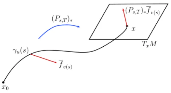
x0 γu(s) f_v(s) (Ps,T)∗ (Ps,T)∗fv(s) x TxM

Figure 1. Differential of the end-point map.

Proposition2.9. The differential of Ex0,T atu∈ U, i.e. DuEx0,T :L

∞_([0_{, T}_]_,_Rk₎ →TxM, where x=γu(T), is (2.6) DuEx0,T(v) = Z T 0 (Ps,T)∗fv(s)(γu(s))ds, ∀v∈L∞([0, T],Rk).

In other words the differentialDuEx0,T applied to the controlv computes the integral mean of the linear part fv(t) of the vector fieldfv(t) along the trajectory defined by u, by pushing it forward to the final point of the trajectory through the flowPs,T (see Fig. 1).

More explicitly,f(x, u) =f0(x) +Pk_i₌₁uifi(x), and Eq. (2.6) is rewritten as follows

DuEx0,T(v) = Z T 0 k X i=1 vi(s)(Ps,T)∗fi(γu(s))ds, ∀v∈L∞([0, T],Rk).

2.3. Lagrange multipliers rule

Fixx0, x∈M. The problem of finding the infimum of the costJT for all admissible curves connecting

the endpointsx0andx, respectively, in timeT, can be naturally reformulated via the end-point map as a constrained extremal problem

(2.7) ST(x0, x) = inf{JT(u)|Ex0,T(u) =x}= inf

E−1

x0,T(x)

JT.

Definition2.10. We say thatu_{∈ U} is anoptimal control if it is a solution of Eq. (2.7).

Remark2.11. Whenf is not injective, a curveγ may be associated with multiple controls.

Never-theless, among all the possible controlsuassociated with the same admissible curve, there exists a unique

controlu∗ which, for a.e. t∈[0, T], minimizes the Lagrangian function. Then, since we are interested in

optimal controls, we assume that any admissible curveγ is always associated with the controlu∗ which

minimizes the Lagrangian, and in this way we have a one-to-one correspondence between admissible curves and controls. With this observation, we say that the admissible curveγ is anoptimal trajectory

(orminimizer) if the associated controlu∗_{is optimal according to Definition 2.10.} Notice that, in general, DuEx0,T is not surjective and the set E

−1

x0,T(x) ⊂ M is not a smooth submanifold. The Lagrange multipliers rule provides a necessary condition to be satisfied by a controlu

which is a constrained critical point for (2.7).

Proposition2.12. Let u∈ U be an optimal control, withx=Ex0,T(u). Then (at least) one of the

two following statements holds true

(i) _∃λT ∈Tx∗M s.t. λTDuEx0,T =duJT, (ii) _∃λT ∈Tx∗M, λT 6= 0,s.t. λTDuEx0,T = 0,

whereλTDuEx0,T denotes the composition of linear maps

L∞_([0_{, T}_]_,_Rk₎ duJT ( ( ❘ ❘ ❘ ❘ ❘ ❘ ❘ ❘ ❘ ❘ ❘ ❘ ❘ ❘ ❘ DuEx0,T / /_T xM λT R

(17)

Definition2.13. A controlu, satisfying the necessary conditions for optimality of Proposition 2.12, is called normal in case (i), while it is called abnormal in case (ii). We use the same terminology to classify the associated extremal trajectoryγu.

Notice that a single control u ∈ U can be associated with two different covectors (or Lagrange multipliers) such that both (i) and (ii) are satisfied. In other words, an optimal trajectory may be simultaneously normal and abnormal. We now introduce a key definition for what follows.

Definition 2.14. A normal extremal trajectoryγ: [0, T]_→M is calledstrictly normal if it is not abnormal. Moreover, if for all s _∈ [0, T] the restriction γ_|[0,s] is also strictly normal, then γ is called

strongly normal.

Remark2.15. A trajectory is abnormal if and only if the differentialDuEx0,T is not surjective. By linearity of the integral, it is easy to show from Eq. (2.6) that this is equivalent to the relation

span_{(Ps,T)∗Dγ(s), s∈[0, T]} 6=Tγ(T)M.

In particularγis strongly normal if and only if a short segmentγ|[0,ε]is strongly normal, for someε≤T.

2.4. Pontryagin Maximum Principle

In this section we recall a weak version of the Pontryagin Maximum Principle (PMP) for the optimal control problem, which rewrites the necessary conditions satisfied by normal optimal solutions in the Hamiltonian formalism. In particular it states that every normal optimal trajectory of problem (2.2) is the projection of a solution of a fixed Hamiltonian system defined onT∗_M_.

Let us denote byπ:T∗_M _→_M _{the canonical projection of the cotangent bundle, and by}_h_{λ, v}_i_the pairing between a cotangent vectorλ_∈T∗

xM and a vectorv∈TxM. The Liouville 1-formς∈Λ1(T∗M)

is defined as follows: ςλ =λ◦π∗, for every λ∈T∗M. The canonical symplectic structure onT∗M is

defined by the non degenerate closed 2-formσ=dς. In canonical coordinates (p, x)_∈T∗_M _{one has}

ς = n X i=1 pidxi, σ= n X i=1 dpi∧dxi.

We denote by ~h the Hamiltonian vector field associated with a function h _∈ C∞₍_T∗_M_{). Namely,}

dλh=σ(·,~h(λ)) for everyλ∈T∗M and the coordinates expression of~his

~h= n X i=1 ∂h ∂pi ∂ ∂xi − ∂h ∂xi ∂ ∂pi .

Let us introduce the smooth control-dependent Hamiltonian onT∗M:

H(λ, u) =_hλ, f(x, u)_{i −}L(x, u), λ_∈T∗M, x=π(λ).

Assumption (A2) guarantees that, for each λ _∈ T∗_M_{, the restriction} _u _{7→ H}₍_{λ, u}_{) to the fibers of} _U has a unique maximum ¯u(λ). Moreover, the fiber-wise strong convexity of the Lagrangian and an easy application of the implicit function theorem prove that the map λ_7→u¯(λ) is smooth. Therefore, it is well defined themaximized Hamiltonian (or simply,Hamiltonian)H :T∗_M _→_R

H(λ)= max.

v∈UxH

(λ, v) =_H(λ,u¯(λ)), λ_∈T∗M, x=π(λ).

Remark 2.16. When f(x, u) = f0(x) +P_ik₌₁uifi(x) is written in a local frame, then ¯u= ¯u(λ) is

characterized as the solution of the system

(2.8) ∂H ∂ui (λ, u) =_hλ, fi(x)i − ∂L ∂ui (x, u) = 0, i= 1, . . . , k.

Theorem 2.17 (PMP, [AS04,PBGM69]). The admissible curve γ : [0, T] → M is a normal extremal trajectory if and only if there exists a Lipschitz lift λ: [0, T]_→T∗_M_{, such that}_γ₍_t_{) =}_π₍_λ₍_t₎₎

and

˙

λ(t) =_H~₍_λ₍_t₎₎_, _t_∈_[0_{, T}_]_.

In particular, γ and λ are smooth. Moreover, the associated control can be recovered from the lift as

u(t) = ¯u(λ(t)), and the final covector λT = λ(T) is a normal Lagrange multiplier associated with u,

(18)

Thus, every normal extremal trajectory γ : [0, T] →M can be written as γ(t) = π◦et ~H(λ0), for

some initial covectorλ0 ∈T∗M (although it may be non unique). This observation motivates the next definition. For simplicity, and without loss of generality, we assume that_H~ _{is complete.}

Definition 2.18. Fix x0 ∈ M. The exponential map with base point x0 is the map Ex0 : R +

×

T∗

x0M →M, defined byEx0(t, λ0) =π◦e

t ~H₍_λ_0).

When the first argument is fixed, we employ the notation_Ex0,t : T ∗

x0M → M to denote the expo-nential map with base pointx0 and timet, namelyEx0,t(λ) =Ex0(t, λ). Indeed, the exponential map is smooth.

From now on, we call geodesic any trajectory that satisfies the normal necessary conditions for

optimality. In other words, geodesics are admissible curves associated with a normal Lagrange multiplier or, equivalently, projections of integral curves of the Hamiltonian flow.

2.5. Regularity of the value function

The next well known regularity property of the value function is crucial for the forthcoming sections (see Definition 2.4).

Theorem 2.19. Let γ: [0, T]→M′ be a strongly normal trajectory. Then there exist ε >0 and an open neighbourhood U ⊂(0, ε)×M′×M′ such that:

(i) (t, γ(0), γ(t))∈U for all t∈(0, ε),

(ii) For any(t, x, y)∈U there exists a unique (normal) minimizer of the cost functionalJt, among

all the admissible curves that connectxwithy in timet, contained in M′,

(iii) The value function(t, x, y)7→St(x, y)is smooth onU.

According to Definition 2.4, the functionS, and henceforth U, depend on the choice of a relatively compactM′ _⊂_M_{. For different relatively compacts, the correspondent value functions} _S _{agree on the} intersection of the associated domainsU: they define the same germ.

The proof of this result can be found in Appendix A. We end this section with a useful lemma about the differential of the value function at a smooth point.

Lemma 2.20. Let x0, x∈ M and T >0. Assume that the function x7→ST(x0, x) is smooth at x

and there exists an optimal trajectory γ: [0, T]_→M joiningx0 tox. Then

(i) γis the unique minimizer of the cost functionalJT, among all the admissible curves that connect

x0 withxin timeT, and it is strictly normal,

(ii) dxST(x0,·) =λT, where λT is the final covector of the normal lift ofγ.

Proof. Under the above assumptions the function

v_7→JT(v)−ST(x0, Ex0,T(v)), v∈L

∞_([0_{, T}_]_,_Rk₎_,

is smooth and non negative. For every optimal trajectoryγ, associated with the controlu, that connects

x0 withxin timeT, one has

0 =du JT(·)−ST(x0, Ex0,T(·)

=duJT −dxST(x0,·)◦DuEx0,T.

Thus,γ is a normal extremal trajectory, with Lagrange multiplier λT =dxST(x0,·). By Theorem 2.17, we can recoverγby the formulaγ(t) =π_◦e(t−T)H~₍_λ

T). Then,γis the unique minimizer ofJT connecting

its endpoints.

Next we show thatγis not abnormal. Fory in a neighbourhood ofx, consider the map Θ :y_7→e−T ~H(dyST(x0,·)).

The map Θ, by construction, is a smooth right inverse for the exponential map at timeT. This implies that xis a regular value for the exponential map and, a fortiori, uis a regular point for the end-point

(19)

CHAPTER 3

Flag and growth vector of an admissible curve

For each smooth admissible curve, we introduce a family of subspaces, which is related with a micro-local characterization of the control system along the trajectory itself.

3.1. Growth vector of an admissible curve

Letγ : [0, T]→M be an admissible, smooth curve such that γ(0) =x0, associated with a smooth

controlu. LetP0,t denote the flow defined byu. We define the family of subspaces ofTx0M (3.1) F_γ(_t)= (. _P₀_,t)−1_∗ D_γ₍_t₎_.

In other words, the familyF_γ(_t) is obtained by collecting the distributions along the trajectory at the initial point, by using the flowP0,t(see Fig. 1).

(P0,t)−_∗1 F_γ_{(0) =}D_x 0 b c b c γ(t) D_γ₍_t₎ x0 F_γ₍_t_{) = (}_P₀_,t₎−1 ∗ Dγ(t)⊂Tx0M

Figure 1. The family of subspacesF_γ(_t).

Given a family of subspaces in a linear space it is natural to consider the associated flag.

Definition3.1. Theflag of the admissible curveγis the sequence of subspaces F_γi(_t)= span. dj dtjv(t) v(t)∈Fγ(t) smooth, j≤i−1 ⊂Tx0M, i≥1. Notice that, by definition, this is a filtration ofTx0M, i.e. F

i

γ(t)⊂Fγi+1(t), for alli≥1.

Definition3.2. Letki(t)= dim. Fγi(t). Thegrowth vector of the admissible curveγis the sequence

of integers_Gγ(t) ={k1(t), k2(t), . . .}.

An admissible curve isample at tif there exists an integer m=m(t) such thatF_γm(t)(_t) =_T_x₀_M. We call the minimalm(t) such that the curve is ample thestep attof the admissible curve. An admissible curve is calledequiregular at t if its growth vector is locally constant at t. Finally, an admissible curve isample (resp. equiregular) if it is ample (resp. equiregular) at each t_∈[0, T].

Remark 3.3. One can analogously introduce the family of subspaces (and the relevant filtration) at any base point γ(s), for every s _∈ [0, T], by defining the shifted curve γs(t) =. γ(s+t). Then

F_γ

s(t)

.

= (Ps,s+t)−1∗ Dγ(s+t). Notice that the relationFγs(t) = (P0,s)∗Fγ(s+t) implies that the growth

vector of the original curve at t can be equivalently computed via the growth vector at time 0 of the curveγt, i.e. ki(t) = dimFγit(0), and Gγ(t) =Gγt(0).

Let us stress that the the family of subspaces (3.1) depends on the choice of the local frame (via the mapP0,t). However, we will prove that the flag of an admissible curve att= 0 and its growth vector (for

all t) are invariant by state-feedback transformation and, in particular, independent on the particular presentation of the system (see Section 3.3).

(20)

Remark 3.4. The following properties of the growth vector of anample admissible curve highlight the analogy with the “classical” growth vector of the distribution.

(i) The functions t _7→ ki(t), for i = 1, . . . , m(t), are lower semicontinuous. In particular, being

integer valued functions, this implies that the set of points t such that the growth vector is locally constant is open and dense on [0, T].

(ii) The function t _7→m(t) is upper semicontinuous. As a consequence, the step of an admissible curve is bounded on [0, T].

(iii) If the admissible curve is equiregular at t, then k1(t) < . . . < km(t) is a strictly increasing

sequence. Let i < m. Ifki(t) =ki+1(t) for allt in a open neighbourhood then, using a local

frame, it is easy to see that this implies ki(t) =ki+1(t) =. . . =km(t) contradicting the fact

that the admissible curve is ample att.

Lemma 3.5. Assume that the curve is equiregular with step m. For every i = 1, . . . , m−1, the derivation of sections ofF_γ(_t) _{induces a linear surjective map on the quotients}

δi:Fγi(t)/Fγi−1(t)−→Fγi+1(t)/Fγi(t), ∀t∈[0, T].

In particular we have the following inequalities for ki= dimFγi(t)

ki−ki−1≤ki+1−ki, ∀i= 1, . . . , m−1.

The proof of Lemma 3.5 is contained in Appendix E. Next, we show how the familyF_γ(_t) can be conveniently employed to characterize strictly and strongly normal geodesics.

Proposition3.6. Let γ: [0, T]→M be a geodesic. Then

(i) γ is strictly normal if and only ifspan_{F_γ(_s)_{, s}_∈[0_{, T}]_}=_T_x 0M, (ii) γ is strongly normal if and only if span_{F_γ(_s)_{, s}_∈[0_{, t}]_}=_T_x

0M for all0< t≤T, (iii) If γ is ample att= 0, then it is strongly normal.

Proof. Recall that a geodesic γ : [0, T] _→M is abnormal on [0, T] if and only if the differential

DuEx0,T is not surjective, which implies (see Remark 2.15)

span_{(Ps,T)∗Dγ(s), s∈[0, T]} 6=Tγ(T)M. By applying the inverse flow (P0,T)−1∗ :Tγ(T)M →Tγ(0)M, we obtain

span_{F_γ(_s)_{, s}_∈[0_{, T}]_{} 6}=_T_x 0M.

This proves (i). In particular, this implies that a geodesic is strongly normal if and only if span_{F_γ₍_s₎_{, s}_∈_[0_{, t}_]_}₌_T_x

0M, ∀0< t≤T,

which proves (ii). We now prove (iii). We argue by contradiction. If the geodesic is not strongly normal, there exists some λ_∈T∗

x0M such thathλ,Fγ(t)i= 0, for all 0< t≤T. Then, by taking derivatives at

t= 0, we obtain that_hλ,Fi

γ(0)i= 0, for alli≥0, which is impossible since the curve is ample at t= 0

by hypothesis.

Remark 3.7. Ample geodesics play a crucial role in our approach to curvature, as we explain in Chapter 4. By Proposition 3.6, these geodesics are strongly normal. One may wonder whether the generic covectorλ0 ∈Tx∗0M corresponds to a strongly normal (or even ample) geodesic. The answer to this question is trivial when there are no abnormal trajectories (e.g. in Riemannian geometry), but the matter is quite delicate in general. For this reason, in order to define the curvature of an affine control system, we assume in the following that the set of ample geodesics is non empty. Eventually, we address the problem of existence of ample geodesics for linear quadratic control systems and sub-Riemannian geometry. In these cases, we will prove that a generic normal geodesic is ample.

3.2. Linearised control system and growth vector

It is well known that the differential of the end-point map at a point u _{∈ U} is related with the linearisation of the control system along the associated trajectory. The goal of this section is to discuss the relation between the controllability of the linearised system and the ampleness of the geodesic.