Archimer

(1)

e note th at this is an aut hor-pr oduc ed PDF of an article a cce pted for publ icatio n foll owin g pe er revi ew. T he defin iti v e pu b lish e r-a uthentic ated ve rsion is av ail a b le on the pub lis her W eb site

Estuarine, Coastal and Shelf Science

Archimer

http://archimer.ifremer.fr

Influence of stability and fragmentation of a worm-reef on benthic macrofauna

Laurent Godeta, b, *, Jérôme Fournierc, Mikaël Jaffréd, Nicolas Desroye

a

CNRS, Laboratoire Géolittomer, UMR 6554 LETG, Université de Nantes, BP 81227, 44312 Nantes cedex 3, France

b

CNRS, UMR 7208 BOREA, Muséum National d’Histoire Naturelle, CRESCO, 38 Rue du Port Blanc, 35800 Dinard, France

c

CNRS, UMR 6042 GEOLAB, Université Blaise Pascal, 4 Rue Ledru, 63057 Clermont-Ferrand cedex 1, France

d

Université de Lille 1, UMR 8187 LOG, Station Marine de Wimereux, 28 Avenue Foch, 62930 Wimereux, France

e

IFREMER, Laboratoire Environnement et Ressources FBN, CRESCO, 38 Rue du Port Blanc, 35800 Dinard, France

*: Corresponding author : Laurent Godet, email address : [email protected]

Abstract :

In coastal areas, reef-builder worms often are bio-engineers by structuring their physical and biological environment. Many studies showed that this engineering role is determined by the densities of the engineer species itself, the highest densities approximately corresponding to the most stable areas from a sedimentological point of view, and hosting the richest and the most diverse benthic fauna. Here, we tested the potential influence of the spatio-temporal dynamics and the spatial fragmentation of one of the largest European intertidal reefs generated by the marine worm Lanice conchilega (Pallas, 1766) (Annelida, Polychaeta) on the associated benthic macrofauna. We demonstrated that the worm densities do have a significant positive role on the abundance, biomass, species richness and species diversity of the benthic macrofauna and that the reef stability also significantly influences the biomass and species diversity. Moreover, the reef fragmentation has significant negative effects on the abundance, biomass and species richness. In addition to L. conchilega densities, the stability and the spatial fragmentation of the reef also significantly structure the associated benthic assemblages. This study demonstrates the interest of “benthoscape ecology” in understanding the role played by marine engineer species from a spatial point of view.

Highlights

► The influence of stability and fragmentation of a worm-reef on benthic macrofauna is tested. ► Stability positively influences biomass and species diversity. ► Fragmentation has negative effects on abundance, biomass and species richness. ► Stability and fragmentation tend to structure benthic assemblages.

(2)

M

A

N

U

S

C

R

IP

T

A

C

E

P

T

E

D

1. Introduction

If landscape ecology has been traditionally restricted to terrestrial systems (Hinchey et al., 2008), few authors have demonstrated the interest of this discipline for marine systems (e.g. Robins and Bell, 1994; 45

Garrabou et al., 1998; Teixidó et al., 2002; Zajac et al., 2003). In 2008, in a special issue of Landscape Ecology on marine and coastal applications in landscape ecology, the interest of this discipline for benthic systems has been highlighted through the concept of “benthoscape ecology” (Zajac, 2008). Benthoscape ecology is an application of Landscape Ecology to the benthic compartment, using remote sensing methods adapted to the marine realm (mainly sonar or aerial photogaphs and satellite imagery 50

for intertidal or shallow-water areas) to identify and delineate different seascape units at the bottom of the ocean. These spatial units are then quantified using geometric or topological indices (MacGarigal et al., 2002) and can be linked with ecological patterns or processes. Such an approach has potential for studying benthic habitats that can be easily mapped and monitored, including intertidal structured habitats (Godet et al., 2009a). Here, we used this method to understand the importance of spatio-55

temporal characteristics on the benthic biodiversity associated with an intertidal worm-reef. Lanice conchilega (Polychaeta, Terebellidae) is a widespread marine species over Europe (Fauvel, 1927; Holthe, 1986) which occurs locally in high densities from a few hundreds to several thousands individuals per square metre (see Buhr and Winter, 1976), both in intertidal and subtidal areas. The habitats structured by L. conchilega are named L. conchilega aggregations (e.g. Zühlke, 60

2001), L. conchilega beds (e.g. Godet et al., 2008) or L. conchilega reefs (e.g. Rabaut et al., 2009). At high densities, the species is considered as an “engineer species” (sensu Jones et al., 1994) because it has a structuring effect both on the physical and the biological compartments (Godet et al., 2008). Above a threshold density, current velocities decrease within the aggregations, deposition of fine sediment particles is facilitated (Friedrichs et al., 2000) and the species produces its own sedimentary structures 65

constituted of mounds and depressions (Carey, 1987; Féral, 1989). The presence of L. conchilega aggregations is also positively correlated with the abundance and the specific richness of the associated macrofauna (Zühlke et al., 1998; Zühlke, 2001; Callaway, 2006; Rabaut et al., 2007; Van Hoey et al., 2008). Rabaut et al. (2007) recently developed the concept of a Russian-doll-like organisation pattern of the associated benthic communities: they found that similarity between individual samples of benthic 70

macrofauna increases as the densities of L. conchilega increase as L. conchilega tends to restructure the species assemblages by expanding the available niche of several species.

Until now, the previous studies on the relationship between this engineer species and its physical and biological environment essentially focused on the influence of the densities of L. conchilega itself. No studies tested the potential influence of the stability of the reefs and their spatial structures on the 75

(3)

M

A

N

U

S

C

R

IP

T

A

C

E

P

T

E

D

associated fauna. In this paper, we tested together the potential influence of: i) L. conchilega densities in the reef, ii) stability of the reef, iii) spatial structures of the reef both on: i) the abundance, biomass, species richness and species diversity of the associated benthic macrofauna, and ii) the structure of the macrozoobenthic assemblages.

80

2. Methods

2.1. Study site

We selected one of the largest intertidal L. conchilega reefs in Europe, located in the Bay of Mont-Saint-85

Michel (BMSM), France (Fig. 1). The Bay is subjected to an extreme megatidal regime (tidal range up to 15.5 m during spring tides). Combined with very low beach slopes, the tides provide large intertidal sandflats, covering more than 250,000 ha. The study was carried out on the main reef of L. conchilega in the BMSM, close to the main reef of Sabellaria alveolata, which is located in the central part of the bay. The sedimentary environment of the bay is mainly controlled by tidal residual current patterns, typically 90

characterized by an anticyclonic gyre off Cancale (NW of the Bay), a large cyclonic gyre around the Channel Islands and reduced drift of water masses to the north along the coast of Normandy. Gyres are partly disrupted under high wind velocity (Bonnot-Courtois et al., 2002). The reef of L. conchilega is located at the edge of the two juxtaposed hydro-sedimentary systems, i.e. where the roughness is

strongest. The central part of the bay is characterized by high bioclastic content (25%-95%) and shows a 95

gradual decrease in mean grain size from the subtidal to the intertidal zone (Bonnot-Courtois et al., 2004; Billeaud et al., 2007). In this area, the tidal flat is mainly formed by very fine sand to coarse carbonate-rich sand, with superficial deposits of silt. Sedimentation rates are higher (3-25 mm.year-1) in the intertidal zones and tend to decrease seawards.

100

# Figure 1 approximately here #

105

2.2. Reef mapping

The reef was mapped on a Geographical Information System (GIS) (Arcview 3.2, ESRI, Redlands, CA, USA) via photo-interpretation processing (see Godet et al., 2008). The 1:10,000 colour aerial

(4)

M

A

N

U

S

C

R

IP

T

A

C

E

P

T

E

D

photographs come from surveys carried out in 1973, 1982, 2002 and 2008 by the French Geographic 110

Institute (IGN). Each date corresponds to a specific map and to a specific layer in the GIS. The high quality of aerial photographs allowed for an accurate manual mapping of the reefs even without geoprocessed methods by an operator with a strong field control based on Ground Control Point acquisition (dGPS). Densities of L. conchilega from ±250 ind.m-2 can be detected on such aerial photographs (Callaway et al., 2010), so that the areas with densities equal or higher to this threshold 115

were mapped as L. conchilega reef. All output maps are to a scale of 1:10,000 even if we zoomed up to 1:1,000 for the mapping process.

2.3. Quantifying stability 120

For a given ecological system, different types of stability can be distinguished (Callaway et al., 2010; modified from Grimm et al., 1999): constancy (the duration a system remains essentially unchanged); resistance (the capacity of a system to remain unchanged despite the presence of disturbance which could potentially change the system); resilience (the property to return to a reference state after a disturbance); and persistence (the property of a system to exist over long periods of time, and, contrary 125

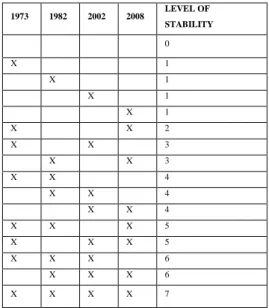
to the constancy, even with intermittent absence). Here, we quantified the stability of the reef through its persistence from 1973 to 2008. The four 1:10,000 maps of the reef (1973, 1982, 2002, 2008) were superimposed as different layers in the GIS to distinguish between seven levels of stability (Tab. 1) resulting in a ‘stability map’. Then, this ‘stability map’ was divided into cells of 1 ha, and for each cell a ‘stability index’ was computed (stability index = % of the cell covering a specific stability level * 130

specific level number). For example, in a cell for which 20% is covered by a stability index of 2 and 80% of a stability index of 5, its stability index will be: 20*2+80*5=440. This index thus ranges

theoretically from 0 (0*0 = no L. conchilega reef present in the cell from 1973 to 2008) to 700 (100*7 = L. conchilega reef covering the full cell in 1973, 1982, 2002 and 2008).

(5)

M

A

N

U

S

C

R

IP

T

A

C

E

P

T

E

D

# Table 1 approximately here #

140

2.4. Quantifying L. conchilega densities

Lanice conchilega densities were examined within the reef in 2005, 2006, 2007 and 2008. Densities were estimated by taking numerical pictures of three 0.25 m-2 random quadrats in the middle of the 1 ha cells of the same grid used to quantify the stability of the reef. The number of intact tube-tops was 145

counted on the pictures; the number of tube-tops is highly correlated with the number of individuals burrowed in the sediment (Ropert and Dauvin, 2000; Strasser and Pieloth, 2001; Zühlke, 2001; Callaway, 2003; Bendell-Young, 2006) and the error associated does not exceed 3% (Ropert, 1999).

2.5. Quantifying spatial structures 150

The spatial structures of the reef were examined with the 2008 map. In this map, two classes were considered: L. conchilega reef and sand. Spatial metrics were calculated only for the L. conchilega class within the cells of the same 1 ha grid used to quantify the stability of the reef. The same process was then performed for three different spatial extents: 0.75 ha, 0.50 ha and 0.25 ha cells (with the same cell 155

centres). For each cell, and for each spatial metric, we calculated a mean metric for the three spatial extents. Calculations of spatial metrics were performed using the public domain software FRAGSTATS version 3.3 (McGarigal et al., 2002). While FRAGSTATS provides a large number of spatial metrics, we selected a subset of them (Table 2). We selected these metrics because: i) they are not correlated with each other, ii) they correspond both to geometric and topologic indices, iii) their interpretation is 160

easy and corresponds to ecological realities.

# Table 2 approximately here # 165

2.6. Sampling, sorting, identifying and weighting benthic macrofauna

Benthic macrofauna was sampled along the same 1 ha grid used to quantify the stability of the reef, but 170

(6)

M

A

N

U

S

C

R

IP

T

A

C

E

P

T

E

D

conchilega densities ≥ 200 ind.m-2 in 2008 (i.e. 80 stations). In each station, one core was collected

(1/40 m-2, 30 cm deep). Benthic samples were sieved in the field through a 1 mm mesh size and the biological material retained was then directly preserved in 4.5% buffered formalin. Once in the laboratory, samples were sorted and macrozoobenthos was identified to the highest taxonomic 175

separation possible, usually species level. The values of the species richness (S), total abundance (N) and species diversity (H’) were calculated from the final macrozoobenthic database, excluding the species L. conchilega itself. Total biomasses were estimated by weighting their dry weight (60°C for 48 h). The ash-free dry weight (AFDW) was calculated as a difference between the dry weight and the ashes (500°C for 3 h).

180

2.7. Statistical analysis

All the statistical analyses were performed with R version 2.10.0 (R Development Core Team, 2009). The relation between i) biodiversity indices (abundance, biomass, species richness and species 185

diversity of the benthic macrofauna), and ii) L. conchilega densities, spatio-temporal index, and spatial metrics, were analysed with multiple linear regression models. The best linear models were selected with the “regsubsets” function of the R package “leaps” which plots a measure of fit against subset size (see Miller, 2002). In other words, regsubsets is an algorithm that enables to select the best combination of factors that best ‘explains’ the variance of a variable.

190

To test the influence of L. conchilega densities, spatio-temporal index, and spatial metrics on macrozoobenthic assemblages, we used the R “MASS” and “vegan” packages. After a log(x+1)

transformation of the macrozoobenthic matrix, non-metric multidimensional scaling ordinations (nMDS) were performed after a computation of a Bray-Curtis similarity matrix, using the “metaMDS” function of the “MASS” packages (Oksanen, 2009). The “envfit” function (“vegan” package) was used to test the 195

influence L. conchilega densities (log (x+1) transformed, as macrozoobenhtic abundances), spatio-temporal index and spatial metrics of the macrozoobenthic asemblages (Oksanen, 2009). Factors were then plotted on the nMDS with the function “ordisurf” of the “vegan” package (Oksanen, 2009).

3. Results

200

3.1. Spatial and biological characteristics of the reef

In 2008, the reef covered 105 ha (Fig.2), 134 ha in 1973, 68 ha in 1982, 193 ha in 2002. The mean L.

conchilega densities from 2005 to 2008 were 1311.71 ind.m-2 (± sd 1411.78), and maximal densities of

(7)

M

A

N

U

S

C

R

IP

T

A

C

E

P

T

E

D

6700 ind.m-2 were reached in the middle of the reef in 2007. The stability of the reef is positively correlated with the L. conchilega densities (R²: 0.33, 316 DF, p: < 0.0001) and the most stable parts of the reef are located approximately in the core area and vice versa (Fig. 2). Only one cell has a stability index of 0 (i.e. no L. conchilega present during the period).

210

# Figure 2 approximately here #

A total of 13806 macroinvertebrates representing 61 different species were recorded. The mean 215

biomass is 49.69 g AFDW.m-2 (± sd 50.43) including the species L. conchilega, and 26.81 g AFDW.m-2 (± sd 36.22) without the species L. conchilega. One single benthic assemblage was identified (average similarity of the assemblage based on a Bray-Curtis similarity matrix, after a log(x+1) transformation: 49.70%), dominated by the two bivalve species Macoma balthica (occurrence: 100%) and

Cerastoderma edule (70%), and the two polychaetes Nephtys hombergii (96%) and L. conchilega (90%). 220

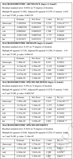
3.2. Influence of reef stability and spatial characteristics of the reef on the macrozoobenthic biodiversity

Lanice conchilega densities are positively correlated with macrozoobenthic abundance, biomass, species richness and diversity (Table 3). Reef stability is positively correlated with macrozoobenthic species 225

diversity, and negatively correlated with biomass. Patch density is negatively correlated with macrozoobenthic abundance, biomass and species richness.

# Table 3 approximately here # 230

3.3. Influence of stability and spatial characteristics of the reef on the macrozoobenthic assemblage structure

235

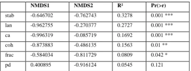
The fitting factors (R²>0.25) most explaining the macrozoobenthic assemblage structure are the stability of the reef, L. conchilega densities, then the total area index (R²=0.17), the cohesion index (R²=0.16), and, finally, the fractal dimension index (R²=0.08) (Figure 3; Table 4).

(8)

M

A

N

U

S

C

R

IP

T

A

C

E

P

T

E

D

240

# Figure 3 approximately here # # Table 4 approximately here #

4. Discussion

245

4.1. Dense, stable and non-fragmented reefs host a higher biodiversity

The first new result comes from the positive effect of the stability of the reef on the species richness. This agrees with Zühlke (2001), Toupoint et al. (2008) and Godet et al. (2009b) demonstrating the low 250

resilience of the macrozoobenthic assemblages associated with L. conchilega reefs. However, regression or disappearance of L. conchilega reefs - even for a short time - involves a rapid biodiversity loss, even if benthic fauna is able to recover quickly after a perturbation of a L. conchilega reef (Rabaut et al., 2008; Callaway et al., 2010). These previous studies had suggested that the biodiversity associated to the reef could be controlled by the stability of the reef itself, and probably more by the constancy of the reef 255

(i.e. the duration a system remains essentially unchanged) than its persistence (i.e. the property of a system to exist over long periods of time, and, contrary to the constancy, even with intermittent absence). However, assessing the constancy of the reef requires a constant monitoring of the reef over time to be able to detect any potential modification or disapearance of the reef, an almost impossible task. Hence, in our study, we used persistence as a proxy for the general stability of the reef as it is 260

almost the only index that can be assessed using remote sensing methods (aerial photographs in our study). We expect that long-term persistence of the reef is highly correlated with long-term constancy of the reef as the most stable areas over long-term period are also likely to be the most stable over short-term periods. In the future, in addition to inter-annual persistence, it would be also interesting to assess the potential effects of the intra-annual persistence (seasonal changes) of the reef on benthic fauna. 265

The second new result is the negative influence of patch densities on the macrozoobenthic abundance, biomass and species richness. Patch densities can be viewed as a proxy of the reef

fragmentation which is thus negative for the benthic macrofauna. This result has to be explored more thoroughly, in the context of a rapid development of human activities fragmenting L. conchilega reefs in European coastal areas. Beam-trawling (Rabaut et al., 2008) and clam cultivation (Toupoint et al., 2008; 270

Godet et al., 2009b) are among human activities for which negative impacts on the fauna associated to L. conchilega reefs have been demonstrated. Such activities leading to a spatial fragmentation can thus also have an impact on non-directly impacted L. conchilega reefs by fragmenting them.

(9)

M

A

N

U

S

C

R

IP

T

A

C

E

P

T

E

D

An unexpected result is the negative influence of the stability of the reef on the biomass although an additional analysis showed that this effect is mainly due to Cerastoderma edule biomass. By

275

excluding C. edule from the total biomass we found no significant relation between the stability of the reef and macrozoobenthic biomass. The sampled C. edule corresponded to juveniles, which can form very mobile aggregations. In the Wadden Sea, Zühlke et al. (1998) also showed that the only

macrofaunal species whose densities were not linked with L. conchilega aggregations was another species of bivalve (Mya arenaria), at a juveline stage.

280

4.2. Reef stability and benthoscape structures have a structuring effect on benthic assemblages

The structuring effect of L. conchilega on benthic fauna was demonstrated by several authors (Zühlke et al., 1998; Zühlke, 2001; Callaway, 2006; Rabaut et al., 2007; Van Hoey et al., 2008). Here, we

285

highlighted that the stability of the reef can have a more structuring effect on benthic assemblages than L. conchilega densities. The other factors best explaining macrozoobenthic assemblages are mainly the total area index and the cohesion index, positively explaining the homogeneity of the assemblages. The most stable, dense, extended and cohesive parts of the reef thus host the most homogeneous

assemblages. 290

4.3. Comparison with other benthic structured habitats

The positive effect of tube-building polychaete aggregations on benthic fauna is a well-known phenomenon, demonstrated for other species, such as Owenia fusiformis (Fager, 1964; Somaschini, 295

1993; Barnay, 2003) or Diopatra cuprea (Woodin, 1978). However, to our knowledge, Dubois et al. (2002) were the only authors demonstrating an effect of three discrete spatial structures of a worm reef on the associated fauna (corresponding to three stages of the reef evolution: degraded reef stage, ball-shaped structures, platform stage). Thus, the quantification of benthoscape structures and their influence on the associated fauna applied to coastal worm-reefs is new.

300

In addition to kelp beds (e.g. Dayton, 1994), coral reefs (e.g. Aronson and Precht, 1995;

Murdoch and Aronson, 1999; Grober-Dunsmore et al., 2008), mussel and oyster beds (DeAlteris, 1988; Smith et al., 2001), the major biogenic habitats studied from a benthoscape perspective concerned seagrass habitats (see the review of Boström et al., 2006). However, it is very difficult to compare our results on worm-reefs with the results obtained on seagrass. According to Boström et al. (2006) no clear 305

patterns emerged when seagrass habitat patch size were tested among the most studied faunal groups, and seagrass habitat fragmentation effects on decapods, bivalves and fish have been inconclusive.

(10)

M

A

N

U

S

C

R

IP

T

A

C

E

P

T

E

D

Coastal worm reefs, such as L. conchilega reefs, but also those generated by Sabellaria alveolata, S. spinulosa or Serpula vermicularis seem to be convenient models to understand the influence of spatial characteristics of aggregative engineer species on the associated fauna. 310

Consequently, contrary to soft-sediment benthoscapes without biogenic patches that are difficult to map and define (Zajac, 1999), such structured habitats can be easily mapped, monitored and their spatial structures can be easily quantified.

5. Conclusions

315

This study provides first results on the application of benthoscape ecology to worm reefs and highlights the importance of stable and non-fragmented parts of the studied reef for macrozoobenthic biodiversity. However, these results cannot be directly generalised for all types of coastal worm reefs and this

approach should be also tested in the future on subtidal reefs (including subtidal L. conchilega reefs, the 320

species being rather subtidal), less dense reefs or on other reef-building species. Benthoscape ecology applied to such coastal habitats is a promising approach in a conservation perspective. Yet, it enables to select the best areas to be conserved, including for example the most stable or less fragmented parts of a reef, and the quantification of the stability of L. conchilega aggregations is one of the key points to classify them as biogenic reefs (see Rabaut et al., 2009; Callaway et al., 2010). It may justify their 325

potential conservation in Europe (European Commission DG Environment, 2003, 2006 and 2007) as, from a conservation perspective, long-lived and stable biogenic concretions should have a greater value than comparable ephemeral habitats (Callaway et al., 2010). Moreover, benthoscape ecology approach is a suitable methodology to better investigate the indirect impacts of human activities on the

fragmentation of coastal habitats. In the future, it would be of value to test for the potential effects of 330

stability and spatial structures of structured coastal habitats: i) at different time scales to understand how temporal changes in spatial structures may influence biodiversity, ii) at different spatial scales and different taxonomic groups to assess how different species may be influenced by different fragmentation levels at different spatial scales. Moreover, the influence of spatial structures of coastal habitats could be investigated in the future on functional diversity, this component of biodiversity being recently

335

investigated for the macrozoobenthic compartment (see Bremner, 2008). Finally, it would also be of value to test the potential effects of 3D benthoscape structures of structured coastal habitats, for example using accurate remote sensing tools such as the LIDAR (Noernberg et al., 2010).

(11)

M

A

N

U

S

C

R

IP

T

A

C

E

P

T

E

D

6. Acknowledgements

Thanks to all volunteers who helped us for field sampling: Amélia Curd, Jézabel Lamoureux, Alexandre Carpentier, Matthieu Beaufils, Christophe Boinet, Julien Guillaudeau and Sébastien Provost. Special 345

thank to Amélia Curd for improving the English of this manuscript and Pierre Godet for helpful comments on a first vesion of this manuscript.

7. References

350

Aronson, R.B., Precht, W.F., 1995. Landscape patterns of reef coral diversity: a test of the

intermediate disturbance hypothesis. Journal of Experimental Marine Biology and Ecology 192, 1-14. Barnay, A.S., 2003. Structure des peuplements de sables fins plus ou moins envasés en Manche: échelles spatiales et biodiversité. PhD thesis, Paris VI University, Paris, France, 250 pp.

Bell, S.S., Fonseca, M.S., Kenworthy, W.J., 2008. Dynamics of a subtropical seagrass landscape: 355

links between disturbance and mobile seed banks. Landscape Ecology 23, 67-74.

Bendell-Young, L., 2006. Contrasting the community structure and select geochemical characteristics of three intertidal regions in relation to shellfish farming. Environmental Conservation 33, 21-27.

Billeaud, I., Tessier, B., Lesueur, P., Caline, B., 2007. Preservation potential of highstand coastal sedimentary bodies in a macrotidal basin: example from the Bay of Mont-Saint-Michel, NW, France. 360

Sedimentary Geology 202, 754-775.

Bonnot-Courtois, C., Caline, B., L’Homer, A., Le Vot, M., 2002. The Bay of Mont-Saint-Michel and the Rance Estuary, recent development and evolution of depositional environments. Mémoire 26, CNRS, EPHE, TotalFinaElf, Pau, 256 p.

Bonnot-Courtois, C., Fournier, J., Dréau, A., 2004. Recent morphodynamics of shell banks in the 365

western part of Mont-Saint-Michel Bay (France). Géomorphologie: Relief, Processus, Environnement 1, 65-80.

Boström, C., Jackson, E.L., Simenstad, C.A., 2006. Seagrass landscapes and their effects on associated fauna: a review. Estuarine, Coastal and Shelf Science 68, 383-403.

Bremner, J. 2008. Species’ traits and ecological functionning in marine conservation and 370

management. Journal of Experimental Marine Biology and Ecology 366, 37-47.

Buhr, K.J., Winter, J.E., 1976. Distribution and maintenance of a Lanice conchilega association in the Weser Estuary (FRG) with special reference to suspension-feeding behaviour of Lanice conchilega. In: Keegan, B.F., Ceidigh, P.A., Boaden, P.J.S. (Eds.), Biology of benthic organisms. Pergamon Press, Oxford, pp. 101-113.

(12)

M

A

N

U

S

C

R

IP

T

A

C

E

P

T

E

D

Callaway, R., 2003. Juveniles stick to adults: recruitment of the tube-dwelling polychaete Lanice conchilega (Pallas, 1766). Hydrobiologia 503, 121-130.

Callaway, R., 2006. Tube worms promote community change. Marine Ecology Progress Series 308, 49-60.

Callaway, R., Desroy, N., Dubois, S., Fournier, J., Frost, M., Godet, L., Hendrick, V.J., Rabaut, M., 380

2010. Ephemeral bio-engineers or reef building polychaetes: how stable are aggregations of the tube worm Lanice conchilega (Pallas, 1766)? Integrative and Comparative Biology 50, 237-250.

Carey, D.A., 1987. Sedimentological effects and palaecological implications of the tube-building polychaete Lanice conchilega Pallas. Sedimentology 34, 49-66.

Dayton, P.K., 1994. Community landscape: scale and stability in hard bottom marine communities. 385

In: Giller, P.S., Hildrew, A.G., Raffaelli, D.G. (Eds.), Aquatic ecology: scales, patterns and processes. Blackwell, Oxford, pp. 289-332.

DeAlteris, J.T., 1998. Application of hydroacoustics to the mapping of subtidal oyster reefs. Journal of Shellfish Research 7, 41-45.

Dubois, S., Retière, C., Olivier, F., 2002. Biodiversity associated with Sabellaria alveolata 390

(Polychaeta: Sabellariidae) reefs: effects of human disturbances. Journal of the Marine Biological Association of the United Kingdom 82, 817-826.

Fager, E.W., 1964. Marine sediments: effects of a tube-building polychaete. Science 143, 356-359. Fauvel, P., 1927. Polychètes sédentaires. Faune de France 16, Paris, France, 494 pp.

Féral, P., 1989. Influence des populations de Lanice conchilega (Pallas) (annélide polychète) sur la 395

sédimentation sableuse intertidale de deux plages bas-normandes (France). Bulletin de la Société Géologique de France 8, 1193-1200.

Friedrichs, M., Graf, G., Springer, B., 2000. Skimming flow induced over a simulated polychaete tube lawn at low population densities. Marine Ecology Progress Series 192, 219-228.

Garrabou, J., Riera, J., Zabal, M., 1998. Landscape pattern indices applied to Mediterranean subtidal 400

rocky benthic communities. Landscape Ecology 13, 225-247.

Godet, L., Fournier, J., Toupoint, N., Olivier, F., 2009a. Mapping and monitoring intertidal benthic habitats: a review of techniques and a proposal for a new visual methodology for the European coasts. Progress in Physical Geography 33(3), 378-402.

Godet, L., Toupoint, N., Fournier, J., Le Mao, P., Retière, C., Olivier, F., 2009b. Clam farmers and 405

oystercatchers: effects of the degradation of Lanice conchilega beds by shellfish farming on the spatial distribution of shorebirds. Marine Pollution Bulletin 58, 589-595.

(13)

M

A

N

U

S

C

R

IP

T

A

C

E

P

T

E

D

Godet, L., Toupoint, N., Olivier, F., Fournier, J., Retière, C., 2008. Considering the functional value of common marine species as a conservation stake: the case of sandmason worm Lanice conchilega (Pallas 1766) (Annelida, Polychaeta) beds. Ambio 37, 347-355.

410

Grimm, V., Bietz, H., Guenther, C.P., Hild, A., Villbrandt, M., Niesel, V., Schleier, U., Dittmann, S., 1999. Stability Properties in the Wadden Sea. In: Dittman, S. (Ed.), The Wadden Sea ecosystem:

stability properties and mechanism. Springer-Verlag, Berlin Heidelberg New York, p. 307.

Grober-Dunsmore, R., Frazer, T.K., Beets, J.P., Lindberg, W.J., Zwick, P., Funicelli, N.A., 2008. Influence of landscape structure on reef fish assemblages. Landscape Ecology 23, 37-53.

415

Hinchey, E.K., Nicholson, M.C., Zajac, R.N., Irlandi, E.A., 2008. Marine and coastal applications in landscape ecology. Landscape Ecology, 23, 1-5.

Holthe, T., 1986. Polychaeta terebellomorpha. Marine Invertebrates of Scandinavia 7. Norwegian University Press, Tøyen, 194 pp.

Jones, C.G., Lawton, J.H., Shachak, M., 1994. Organisms as ecosystem engineers. Oikos 69, 373-420

386.

McGarigal, K., Cushman, S.A., Neel, M.C., Ene, E., 2002. FRAGSTATS: Spatial Pattern Analysis Program for Categorical Maps. Computer software program produced by the authors at the University of Massachusetts, Amherst. Available at the following web site:

http://www.umass.edu/landeco/research/fragstats/fragstats.html. 425

Miller, A., 2002. Subset Selection in Regression, 2nd edn. Chapman et Hall, London.

Murdoch, T.J.T., Aronso, R.B., 1999. Scale-dependant spatial variability of coral assemblages along the Florida Reef Tract. Coral Reefs 18, 341-351.

Noernberg, M., Fournier, J., Dubois, S., Populus, J., 2010. Using airborne laser altimetry to estimate Sabellaria alveolata (L.) (Polychaeta: Sabellariidae) reefs volume in tidal flat environment. Estuarine, 430

Coastal and Shelf Science 90, 93-102.

Oksanen, J., 2009. Mutlivariate Analysis of Ecological Communities in R: vegan tutorial, 42 pp. R Development Core Team, 2009. R: A language and environment for statistical computing. R Foundation for Statistical Computing, Vienna, Austria. http://www.R-project.org.

Rabaut, M., Braeckman, U., Hendrickx, F., Vincx, M., Degraer, S., 2008. Experimental beam-435

trawling in Lanice conchilega reefs: Impact on the associated fauna. Fisheries Research 90, 209-216. Rabaut, M., Guilini, K., Van Hoey, G., Vincx, M., Degraer, S., 2007. A bio-engineered soft-bottom environment: the impact of Lanice conchilega on the benthic species-specific densities and community structure. Estuarine, Coastal and Shelf Science 75, 525-536.

Rabaut, M., Vincx, M., Degraer, S., 2009. Do Lanice conchilega (sandmason) aggregations classify 440

(14)

M

A

N

U

S

C

R

IP

T

A

C

E

P

T

E

D

Robins, B.D., Bell, S.S., 1994. Seagrass landscapes: a terrestrial approach to the marine subtidal environment. Trends in Ecology and Evolution 9, 301-303.

Ropert, M., 1999. Caractérisation et déterminisme du développement d’une population de l’annélide tubicole Lanice conchilega (Pallas, 1766) (Polychète Terebellidae) associé à la conchyliculture en Baie 445

des Veys (Baie de Seine Occidentale). PhD thesis, French Museum of Natural History, Paris, France, 172 pp.

Ropert, M., Dauvin, J.C., 2000. Renewal and accumulation of a Lanice conchilega (Pallas) population in the bale des Veys, western Bay of Seine. Oceanologica Acta 23, 529-546.

Smith, T.B., Bruce, D.G., Roach, E.B., 2001. Remote acoustic habitat assessment techniques used to 450

characterize the quality and extent of oyster bottom in the Chesapeake Bay. Marine Geodesy 24, 171-189.

Somaschini, A., 1993. A Mediterranean fine-sand polychaete community and the effect of the tube-dwelling Owenia fusiformis (Delle Chiaje) on community structure. Internationale Revue der Gesamte Hydrobiologie 78, 219-233.

455

Strasser, M., Pieloth, U., 2001. Recolonization pattern of the polychaete Lanice conchilega on an intertidal sand flat following the severe winter of 1995/96. Helgoland Marine Research 55, 176-181.

Teixidó, N., Garrabou, J., Arntz, W.E., 2002. Spatial pattern quantification of Antarctic benthic communities using landscape indices. Marine Ecology Progress Series 242, 1-14.

Toupoint, N., Godet, L., Fournier, J., Retière, C., Olivier, F., 2008. Does Manila clam cultivation 460

affect habitats of the engineer species Lanice conchilega (Pallas, 1766)? Marine Pollution Bulletin 56, 1429-1438.

Van Hoey, G., Guilini, K., Rabaut, M., Vincx, M., Degraer, S., 2008. Ecological implications of the presence of the tube-building polychaete Lanice conchilega on soft-bottom benthic ecosystems. Marine Biology 154, 1009-1019.

465

Woodin, S.A., 1978. Refuges, disturbance, and community structure: a marine soft-bottom example. Ecology 59, 274-284.

Zajac, R.N., 1999. Understanding the seafloor landscape in relation to assessing and managing impacts on coastal environments. In: Gray, J.S., Ambrose, W. Jr, Szaniawska, A. (Eds.), Biochemical cycling and sediment ecology. Kluwer Publishing, Dodrecht, pp. 211-227.

470

Zajac, R.N., 2008. Challenges in marine, soft-sediment benthoscape ecology. Landscape Ecology 23, 7-18.

Zajac, R.N., Lewis, R.S., Poppe, L.J., Twichell, D.C., Vozarik, J., Di-Giacomo-Cohen, M., 2003. Responses of infaunal populations to benthoscape patch structures and the potential importance of transition zones. Limnology and Oceanography 48, 829-842.

(15)

M

A

N

U

S

C

R

IP

T

A

C

E

P

T

E

D

Zühlke, R., 2001. Polychaete tubes create ephemeral community patterns, Lanice conchilega (Pallas, 1766) associations studied over six years. Journal of Sea Research 46, 261-272.

Zühlke, R., Blome, D., Heinz Van Bernem, K., Dittmann, S., 1998. Effects of tube-building

polychaete Lanice conchilega (Pallas) on benthic macrofauna. Senckenbergiana Maritima 29, 131-138. 480

(16)

M

A

N

U

S

C

R

IP

T

A

C

E

P

T

E

D

Table 1. Calculation of the stability level of the reef. “X” means that the reef is present.

1973 1982 2002 2008 LEVEL OF STABILITY 0 X 1 X 1 X 1 X 1 X X 2 X X 3 X X 3 X X 4 X X 4 X X 4 X X X 5 X X X 5 X X X 6 X X X 6 X X X X 7 485

(17)

M

A

N

U

S

C

R

IP

T

A

C

E

P

T

E

D

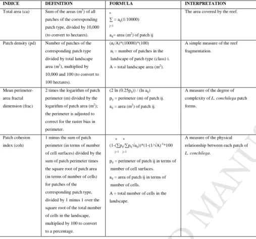
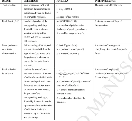
Table 2. Class metrics (n=4) used to quantify the landscape structure of the reef (from McGarigal et al.

2002). 490

INDICE DEFINITION FORMULA INTERPRETATION

Total area (ca) Sum of the areas (m2_{) of all}

patches of the corresponding patch type, divided by 10,000 (to convert to hectares).

n

∑ = aij(1/10000) j=1

aij= area (m2) of patch ij

The area covered by the reef.

Patch density (pd) Number of patches of the corresponding patch type divided by total landscape area (m2

), multiplied by 10,000 and 100 (to convert to 100 hectares).

(ni/A)*(10000)*(100)

ni = number of patches in the

landscape of patch type (class) i. A = total landscape area (m2_).

A simple measure of the reef fragmentation.

Mean perimeter-area fractal dimension (frac)

2 times the logarithm of patch perimeter (m) divided by the logarithm of patch area (m2_);

the perimeter is adjusted to correct for the raster bias in perimeter.

(2 ln (0.25pij)) / (ln aij)

pij = perimeter (m) of patch ij.

aij = area (m2) of patch ij.

A measure of the degree of complexity of L. conchilega patch forms.

Patch cohesion index (coh)

1 minus the sum of patch perimeter (in terms of number of cell surfaces) divided by the sum of patch perimeter times the square root of patch area (in terms of number of cells) for patches of the corresponding patch type, divided by 1 minus 1 over the square root of the total number of cells in the landscape, multiplied by 100 to convert to a percentage.

n n

(1-(∑pij/∑pij√aij))*(1-(1/√A)-1*100 j=1 j=1

pij = perimeter of patch ij in terms of

number of cell surfaces. aij = area of patch ij in terms of

number of cells.

A = total number of cells in the landscape.

A measure of the physical relationship between each patch of L. conchilega.

(18)

M

A

N

U

S

C

R

IP

T

A

C

E

P

T

E

D

Table 3. Best regression models for macrozoobenthic abundance, biomass, species richness and

diversity in relation to L. conchilega densities, reef stability and reef spatial structures. 0<p<0.001 (***); 495

0.001<p<0.01 (**); 0.01<p<0.05 (*). lan=mean L. conchilega densities 2005-2008 log(x+1) transf.; stab=stability index; ca=total area; pd=patch density; coh=patch cohesion index.

MACROZOOBENTHIC ABUNDANCE (log(x+1) transf.) Residual standard error: 0.8362 on 75 degrees of freedom

Multiple R-squared: 0.1982, Adjusted R-squared: 0.1555, F-statistic: 4.635 on 4 and 75 DF, p-value: 0.002129

Estimate Std. Error t value Pr(>|t|) (Intercept) 3.1895944 0.5572506 5.724 2.03e-07 *** pd -0.0002356 0.0001011 -2.330 0.02250 * coh 0.0085041 0.0065025 1.308 0.19493 stab -0.0013106 0.0007544 -1.737 0.08646 lan 0.1833671 0.0552522 3.319 0.00140 ** MACROZOOBENTHIC BIOMASS (log(x+1) transf.)

Residual standard error: 0.355 on 75 degrees of freedom

Estimate Std. Error t value Pr(>|t|) (Intercept) 1.280e-01 2.366e-01 0.541 0.59022 pd -9.124e-05 4.294e-05 -2.125 0.03688 * coh 4.111e-03 2.761e-03 1.489 0.14063 stab -9.674e-04 3.203e-04 -3.020 0.00345 ** lan 6.666e-02 2.346e-02 2.842 0.00578 ** MACROZOOBENTHIC SPECIES RICHNESS (log(x+1) transf.) Residual standard error: 0.394 on 74 degrees of freedom

Estimate Std. Error t value Pr(>|t|) (Intercept) 1.585e+00 2.680e-01 5.915 9.54e-08 *** ca -9.125e-01 7.166e-01 -1.273 0.20687 pd -1.346e-04 5.417e-05 -2.484 0.01525 * coh 5.321e-03 3.424e-03 1.554 0.12442 stab 4.228e-04 3.720e-04 1.137 0.25930 lan 7.368e-02 2.630e-02 2.802 0.00648 ** MACROZOOBENTHIC SPECIES DIVERSITY

Multiple R-squared: 0.2548, Adjusted R-squared: 0.2254, F-statistic: 8.662 on 3 and 76 DF, p-value: 5.146e-05

Estimate Std. Error t value Pr(>|t|) (Intercept) 1.004e+00 1.274e-01 7.887 1.81e-11 *** pd -5.571e-05 4.380e-05 -1.272 0.2073 stab 6.940e-04 3.043e-04 2.280 0.0254 * lan 4.913e-02 2.395e-02 2.051 0.0437 *

(19)

M

A

N

U

S

C

R

IP

T

A

C

E

P

T

E

D

Table 4. Factors best explaining macrozoobenthic assemblages.

The first two columns give direction cosines of the vectors, and R² gives the squared correlation 500

coefficient. p values are based on 999 permutations: 0<p<0.001 (***); 0.001<p<0.01 (**); 0.01<p<0.05 (*); 0.05<p<0.1 (.). lan = mean L. conchilega densities 2005-2008; stab = stability index; ca = total area; pd = patch density; coh = patch cohesion index, frac = mean perimeter-area fractal dimension.

NMDS1 NMDS2 R² Pr(>r) stab -0.646702 -0.762743 0.3278 0.001 *** lan -0.962755 -0.270377 0.2727 0.001 *** ca -0.996319 -0.085719 0.1692 0.001 *** coh -0.873883 -0.486135 0.1563 0.01 ** frac -0.584034 -0.811729 0.0809 0.042 * pd 0.400895 -0.916124 0.0545 0.121 505 510 515

(20)

M

A

N

U

S

C

R

IP

T

A

C

E

P

T

E

D

520

(21)

M

A

N

U

S

C

R

IP

T

A

C

E

P

T

E

D

525

Figure 2. Map of the L. conchilega reef, stability, L. conchilega densities and macrozoobenthic

(22)

M

A

N

U

S

C

R

IP

T

A

C

E

P

T

E

D

Figure 3. nMDS plot of the macrozoobenthic abundance data (log(x+1) transformed) obtained in 80

530

samples and based on the Bray-Curtis similarity. Arrows represent the 6 factors significantly explaining the ordination and surface fitting represents the 2 factors best explaining the ordination (R²>0.25). lan = mean L. conchilega densities 2005-2008 (log (x+1) transformed); stab = stability index; ca = total area; pd = patch density; coh = patch cohesion index; frac = mean perimeter-area fractal dimension.

(23)

M

A

N

U

S

C

R

IP

T

A

C

E

P

T

E

D

Table 1. Calculation of the stability level of the reef. “X” means that the reef is present.

1973 1982 2002 2008 LEVEL OF STABILITY 0 X 1 X 1 X 1 X 1 X X 2 X X 3 X X 3 X X 4 X X 4 X X 4 X X X 5 X X X 5 X X X 6 X X X 6 X X X X 7

(24)

M

A

N

U

S

C

R

IP

T

A

C

E

P

T

E

D

Table 2. Class metrics (n=4) used to quantify the landscape structure of the reef (from

McGarigal et al. 2002).

INDICE DEFINITION FORMULA INTERPRETATION

Total area (ca) Sum of the areas (m2_{) of all}

patches of the corresponding patch type, divided by 10,000 (to convert to hectares).

n

∑ = aij(1/10000) j=1

aij= area (m2) of patch ij

The area covered by the reef.

Patch density (pd) Number of patches of the corresponding patch type divided by total landscape area (m2

), multiplied by 10,000 and 100 (to convert to 100 hectares).

(ni/A)*(10000)*(100)

ni = number of patches in the

landscape of patch type (class) i. A = total landscape area (m2_).

A simple measure of the reef fragmentation.

Mean perimeter-area fractal dimension (frac)

2 times the logarithm of patch perimeter (m) divided by the logarithm of patch area (m2_);

the perimeter is adjusted to correct for the raster bias in perimeter.

(2 ln (0.25pij)) / (ln aij)

pij = perimeter (m) of patch ij.

aij = area (m2) of patch ij.

A measure of the degree of complexity of L. conchilega patch forms.

Patch cohesion index (coh)

1 minus the sum of patch perimeter (in terms of number of cell surfaces) divided by the sum of patch perimeter times the square root of patch area (in terms of number of cells) for patches of the corresponding patch type, divided by 1 minus 1 over the square root of the total number of cells in the landscape, multiplied by 100 to convert to a percentage.

n n

(1-(∑pij/∑pij√aij))*(1-(1/√A)-1*100 j=1 j=1

pij = perimeter of patch ij in terms of

number of cell surfaces. aij = area of patch ij in terms of

number of cells.

A = total number of cells in the landscape.

A measure of the physical relationship between each patch of L. conchilega.

(25)

M

A

N

U

S

C

R

IP

T

A

C

E

P

T

E

D

Table 3. Best regression models for macrozoobenthic abundance, biomass, species richness

and diversity in relation to L. conchilega densities, reef stability and reef spatial structures. 0<p<0.001 (***); 0.001<p<0.01 (**); 0.01<p<0.05 (*). lan=mean L. conchilega densities 2005-2008 log(x+1) transf.; stab=stability index; ca=total area; pd=patch density; coh=patch cohesion index.

MACROZOOBENTHIC ABUNDANCE (log(x+1) transf.) Residual standard error: 0.8362 on 75 degrees of freedom

Estimate Std. Error t value Pr(>|t|) (Intercept) 3.1895944 0.5572506 5.724 2.03e-07 *** pd -0.0002356 0.0001011 -2.330 0.02250 * coh 0.0085041 0.0065025 1.308 0.19493 stab -0.0013106 0.0007544 -1.737 0.08646 lan 0.1833671 0.0552522 3.319 0.00140 ** MACROZOOBENTHIC BIOMASS (log(x+1) transf.)

Estimate Std. Error t value Pr(>|t|) (Intercept) 1.280e-01 2.366e-01 0.541 0.59022 pd -9.124e-05 4.294e-05 -2.125 0.03688 * coh 4.111e-03 2.761e-03 1.489 0.14063 stab -9.674e-04 3.203e-04 -3.020 0.00345 ** lan 6.666e-02 2.346e-02 2.842 0.00578 ** MACROZOOBENTHIC SPECIES RICHNESS (log(x+1) transf.) Residual standard error: 0.394 on 74 degrees of freedom

Estimate Std. Error t value Pr(>|t|) (Intercept) 1.585e+00 2.680e-01 5.915 9.54e-08 *** ca -9.125e-01 7.166e-01 -1.273 0.20687 pd -1.346e-04 5.417e-05 -2.484 0.01525 * coh 5.321e-03 3.424e-03 1.554 0.12442 stab 4.228e-04 3.720e-04 1.137 0.25930 lan 7.368e-02 2.630e-02 2.802 0.00648 ** MACROZOOBENTHIC SPECIES DIVERSITY

Multiple R-squared: 0.2548, Adjusted R-squared: 0.2254, F-statistic: 8.662 on 3 and 76 DF, p-value: 5.146e-05

Estimate Std. Error t value Pr(>|t|) (Intercept) 1.004e+00 1.274e-01 7.887 1.81e-11 *** pd -5.571e-05 4.380e-05 -1.272 0.2073 stab 6.940e-04 3.043e-04 2.280 0.0254 * lan 4.913e-02 2.395e-02 2.051 0.0437 *

(26)

M

A

N

U

S

C

R

IP

T

A

C

E

P

T

E

D

Table 4. Factors best explaining macrozoobenthic assemblages.

The first two columns give direction cosines of the vectors, and R² gives the squared correlation coefficient. p values are based on 999 permutations: 0<p<0.001 (***); 0.001<p<0.01 (**); 0.01<p<0.05 (*); 0.05<p<0.1 (.). lan = mean L. conchilega densities 2005-2008; stab = stability index; ca = total area; pd = patch density; coh = patch cohesion index, frac = mean perimeter-area fractal dimension.

NMDS1 NMDS2 R² Pr(>r) stab -0.646702 -0.762743 0.3278 0.001 *** lan -0.962755 -0.270377 0.2727 0.001 *** ca -0.996319 -0.085719 0.1692 0.001 *** coh -0.873883 -0.486135 0.1563 0.01 ** frac -0.584034 -0.811729 0.0809 0.042 * pd 0.400895 -0.916124 0.0545 0.121