Contents lists available at
ScienceDirect
Computers and Mathematics with Applications
journal homepage:
www.elsevier.com/locate/camwa
Hierarchical gradient based iterative parameter estimation algorithm for
multivariable output error moving average systems
✩Zhening Zhang
a
, Feng Ding
a
,∗
, Xinggao Liu
b
aKey Laboratory of Advanced Process Control for Light Industry (Ministry of Education), School of IoT Engineering, Jiangnan University, Wuxi 214122, PR China bState Key Laboratory of Industrial Control Technology, Department of Control Science and Engineering, Zhejiang University, Hangzhou 310027, PR China
a r t i c l e
i n f o
Article history:Received 4 September 2010 Received in revised form 27 November 2010 Accepted 8 December 2010 Keywords: Iterative algorithm Jacobi iteration Matrix equation Gradient search Parameter estimation Iterative identification Hierarchical identification Multivariable OEMA-like model Multivariable CARMA-like model
a b s t r a c t
According to the hierarchical identification principle, a hierarchical gradient based iterative
estimation algorithm is derived for multivariable output error moving average systems
(i.e., multivariable OEMA-like models) which is different from multivariable CARMA-like
models. As there exist unmeasurable noise-free outputs and unknown noise terms in
the information vector/matrix of the corresponding identification model, this paper is, by
means of the auxiliary model identification idea, to replace the unmeasurable variables in
the information vector/matrix with the estimated residuals and the outputs of the auxiliary
model. A numerical example is provided.
©
2010 Elsevier Ltd. All rights reserved.
1. Introduction
Parameter estimation is a basic method for system modelling, signal filtering, adaptive control [1–9]. For example,
Aihara, et al. discussed parameter estimation problems of term structures modeled by stochastic hyperbolic systems [1]
and of stochastic volatility models from stock data using particle filter application to AEX index [2]; Ding, et al. presented
self-tuning control algorithms for nonlinear dual-rate sampled-data systems [7] and for discrete-time systems using the
multi-innovation identification theory [9–17]. The iterative methods are very important for solving matrix equations
[18,19], e.g., the famous Jacobi iteration and the Gauss–Seidel iteration for solving the equation
Ax
=
b
[20–22].
In this literature, Ding, et al. extended the Jacobi iteration and the Gauss–Seidel iteration to general matrix equations
and presented a large family of iterative methods for
Ax
=
b
and
AXB
=
F
[21,22]. Furthermore, they presented a series of
iterative algorithms, e.g., the least squares based iterative algorithms and the gradient based iterative algorithms [21–28]
for (coupled) Sylvester matrix equations and general (coupled) matrix equations, e.g.,
AXB
=
F
.
AX
+
XB
=
F
.
✩This work was supported in part by the National Natural Science Foundation of China (Nos. 60973043 and 50876093), International Cooperation and Exchange Project of Science and Technology (Department of Zhejiang Province, No. 2009C34008), and Zhejiang Provincial Natural Science Foundation for Distinguished Young Scientists (No. R4100133).
∗
Corresponding author.E-mail addresses:[email protected](Z. Zhang),[email protected](F. Ding),[email protected](X. Liu). 0898-1221/$ – see front matter©2010 Elsevier Ltd. All rights reserved.
AX
+
X
TB
=
F
.
AXB
+
CXD
=
F
.
AX
1B
+
CX
2D
=
F
.
A
1XB
1+
A
2XB
2+ · · · +
A
pXB
p=
F
.
A
1XB
1+ · · · +
A
pXB
p+
C
1X
TD
1+ · · · +
C
qX
TD
q=
F
.
A
11XB
11+ · · · +
A
1qXB
1q+
C
11X
TD
11+ · · · +
C
1qX
TD
1q=
F
1,
A
21XB
21+ · · · +
A
2qXB
2q+
C
21X
TD
21+ · · · +
C
2qX
TD
2q=
F
2,
...
A
p1XB
p1+ · · · +
A
pqXB
pq+
C
p1X
TD
p1+ · · · +
C
pqX
TD
pq=
F
p.
A
11XB
11+
A
12XB
12+ · · · +
A
1qXB
1q=
F
1,
A
21XB
21+
A
22XB
22+ · · · +
A
2qXB
2q=
F
2,
...
A
p1XB
p1+
A
p2XB
p2+ · · · +
A
pqXB
pq=
F
p.
A
11X
1B
11+
A
12X
2B
12+ · · · +
A
1qX
qB
1q=
F
1A
21X
1B
21+
A
22X
2B
22+ · · · +
A
2qX
qB
2q=
F
2,
...
A
p1X
1B
p1+
A
p2X
2B
p2+ · · · +
A
pqX
qB
pq=
F
p.
The last five matrix equations were proposed first by Ding and Chen [21,23,24].
The iterative methods are widely used in system identification and parameter estimation, e.g., the least squares based
parameter identification algorithms and gradient based parameter estimation algorithms [29–35].
The hierarchical identification principle is based on the decomposition technique and is very useful in the identification
of multivariable systems [36,37]. Recently, new hierarchical least squares algorithms and hierarchical stochastic gradient
algorithms were developed for multivariable equation error systems using the hierarchical identification principle [36,37].
Xiang, et al. presented a hierarchical least squares algorithm for single-input multiple-output systems based on the auxiliary
model [38]; Han, et al. proposed a hierarchical least squares based iterative identification for multivariable systems with
moving average noises (i.e., multivariable CARMA-like models) [39]. On the basis of the work in [39], this paper studies the
hierarchical gradient based iterative parameter estimation method for multivariable output error moving average systems
using the hierarchical identification principle.
The paper is organized as follows. Section
2
describes the output error moving average system and derives its
identification model. Section
3
derives a hierarchical gradient based iterative parameter identification algorithm for an
OEMA system. Section
4
gives the version of the hierarchical gradient based iterative algorithm with finite measurement
data. Section
5
provides an illustrative example. Finally, concluding remarks are given in Section
6.
2. The system description and identification model
Consider a multivariable output error moving average (OEMA) system (i.e., multivariable OEMA-like models),
y
(
t
)
=
Q
(
z
)
α(
z
)
u
(
t
)
+
D
(
z
)
v
(
t
),
(1)
which is different from the multivariable CARMA-like systems with moving average noises [39], where
y
(
t
)
∈
R
mis the
system output vector,
u
(
t
)
∈
R
ris the system input vector,
v
(
t
)
∈
R
mis a stochastic white noise vector with zero mean
and variance
σ
2,
α(
z
)
is a monic polynomial in the unit backward shift operator
z
−1[
z
−1y
(
t
)
=
y
(
t
−
1
)
]
,
Q
(
z
)
is a matrix
polynomial in
z
−1,
D
(
z
)
is a polynomial in
z
−1, and defined by
α(
z
)
:=
1
+
α
1z
−1+
α
2z
−2+ · · · +
α
nz
−n, α
i∈
R
1,
Q
(
z
)
:=
Q
1z
−1+
Q
2z
−2+ · · · +
Q
nz
−n,
Q
i∈
R
m×r,
D
(
z
)
:=
1
+
d
1z
−1+
d
2z
−2+ · · · +
d
ndz
−nd,
d
i
∈
R
1.
Define the noise-free output,
x
(
t
)
:=
Q
(
z
)
α(
z
)
u
(
t
)
∈
R
m
.
(2)
Substitute
(2)
into
(1)
gives
Eq.
(2)
can be written as
x
(
t
)
+
n−
i=1α
ix
(
t
−
i
)
=
n−
i=1Q
iu
(
t
−
i
),
(4)
or
x
(
t
)
= −
n−
i=1α
ix
(
t
−
i
)
+
n−
i=1Q
iu
(
t
−
i
).
(5)
Substituting
(5)
into
(3), we have
y
(
t
)
+
n−
i=1α
ix
(
t
−
i
)
−
nd−
i=1d
iv
(
t
−
i
)
=
n−
i=1Q
iu
(
t
−
i
)
+
v
(
t
).
(6)
Define the parameter vectors
ϑ
s,
ϑ
nand
ϑ
, the parameter matrix
θ
, the input information vector
ϕ
(
t
)
and the information
matrices
ψ
s(
t
)
,
ψ
n(
t
)
and
ψ
(
t
)
as
ϑ
s:=
[
α
1, α
2, . . . , α
n]
T∈
R
n,
ϑ
n:=
d
1,
d
2, . . . ,
d
nd
T∈
R
nd,
ϑ
:=
[
ϑ
sϑ
n]
∈
R
n+nd,
θ
T:=
[
Q
1,
Q
2, . . . ,
Q
n]
∈
R
m×(nr),
ϕ
(
t
)
:=
u
T(
t
−
1
),
u
T(
t
−
2
), . . . ,
u
T(
t
−
n
)
T∈
R
(nr),
ψ
s(
t
)
:=
[
x
(
t
−
1
),
x
(
t
−
2
), . . . ,
x
(
t
−
n
)
]
∈
R
m×n,
ψ
n(
t
)
:=
[
−
v
(
t
−
1
),
−
v
(
t
−
2
), . . . ,
−
v
(
t
−
n
d)
]
∈
R
m×nd,
ψ
(
t
)
:=
ψ
s(
t
),
ψ
n(
t
)
∈
R
m×(n+nd).
Eq.
(5)
can be rewritten as
x
(
t
)
= −
ψ
s(
t
)
ϑ
s+
θ
Tϕ
(
t
).
(7)
From
(6), we get the following identification model
y
(
t
)
+
ψ
(
t
)
ϑ
=
θ
Tϕ
(
t
)
+
v
(
t
).
(8)
3. The iterative identification algorithm
A difficulty in identification is that there exist the unknown noise vectors
v
(
t
−
i
)
and noise-free output vectors
x
(
t
−
i
)
of the information matrix
ψ
(
t
)
in the identification model in
(8), the solution is to use the decomposition based hierarchical
identification principle in [36,37] to derive the estimation algorithm of the parameter matrix
θ
and the parameter vector
ϑ
.
That is, Eq.
(8)
is decomposed into two virtual subsystems which contain the parameter vector
ϑ
and the parameter matrix
θ
, respectively, and then the parameters of these two subsystems are identified. The basic idea is to replace the unknown
v
(
t
−
i
)
with the estimated residual and the unknown
x
(
t
−
i
)
with the output of an auxiliary model.
Define two intermediate vectors,
b
1(
t
)
:=
θ
Tϕ
(
t
)
∈
R
m,
b
2(
t
)
:=
ψ
(
t
)
ϑ
∈
R
m.
Decompose
(8)
into the following two virtual subsystems
S
1:
y
(
t
)
= −
ψ
(
t
)
ϑ
+
b
1(
t
)
+
v
(
t
),
S
2:
y
(
t
)
=
θ
Tϕ
(
t
)
−
b
2(
t
)
+
v
(
t
).
Consider newest
p
data from
i
=
t
−
p
+
1 to
i
=
t
and define the stacked output vector
Y
1(
t
)
and the stacked matrix
Y
2(
t
)
, the stacked information matrices
ψ
(
t
)
and
Φ
(
t
)
, the stacked white noise vector
V
1(
t
)
and the stacked noise matrix
V
2(
t
)
, and the inner vector
B
1(
t
)
and the inner matrix
B
2(
t
)
as
Y
1(
t
)
:=
y
(
t
)
y
(
t
−
1
)
...
y
(
t
−
p
+
1
)
∈
R
(mp),
Ψ
(
t
)
:=
ψ
(
t
)
ψ
(
t
−
1
)
...
ψ
(
t
−
p
+
1
)
∈
R
(mp)×(n+nd),
B
1(
t
)
:=
b
1(
t
)
b
1(
t
−
1
)
...
b
1(
t
−
p
+
1
)
=
θ
Tϕ
(
t
)
θ
Tϕ
(
t
−
1
)
...
θ
Tϕ
(
t
−
p
+
1
)
∈
R
(mp),
(9)
V
1(
t
)
:=
v
(
t
)
v
(
t
−
1
)
...
v
(
t
−
p
+
1
)
∈
R
(mp),
Y
2(
t
)
:=
[
y
(
t
),
y
(
t
−
1
), . . . ,
y
(
t
−
p
+
1
)
]
∈
R
m×p,
Φ
(
t
)
:=
[
ϕ
(
t
),
ϕ
(
t
−
1
), . . . ,
ϕ
(
t
−
p
+
1
)
]
∈
R
(nr)×p,
B
2(
t
)
:=
[
b
2(
t
),
b
2(
t
−
1
), . . . ,
b
2(
t
−
p
+
1
)
]
=
[
ψ
(
t
)
ϑ
,
ψ
(
t
−
1
)
ϑ
, . . . ,
ψ
(
t
−
p
+
1
)
ϑ
]
∈
R
m×p,
(10)
V
2(
t
)
:=
[
v
(
t
),
v
(
t
−
1
), . . . ,
v
(
t
−
p
+
1
)
]
∈
R
m×p.
Then we have
S
1:
Y
1(
t
)
= −
Ψ
(
t
)
ϑ
+
B
1(
t
)
+
V
1(
t
),
S
2:
Y
2(
t
)
=
θ
TΦ
(
t
)
−
B
2(
t
)
+
V
2(
t
).
Let
‖
X
‖
2:=
tr
[
XX
T]
, define two criterion functions:
J
1(
ϑ
)
= ‖
Y
1(
t
)
+
Ψ
(
t
)
ϑ
−
B
1(
t
)
‖
2,
J
2(
θ
)
= ‖
Y
2(
t
)
−
θ
TΦ
(
t
)
+
B
2(
t
)
‖
2.
Let
k
=
1
,
2
, . . .
be an iteration variable,
ϑ
ˆ
k(
t
)
and
θ
ˆ
k(
t
)
represent the estimates of
ϑ
and
θ
at iteration
k
,
µ
k(
t
)
⩾
0 is the
time-varying iterative step-size (time-varying convergence factor). Minimizing
J
1(
ϑ
)
and
J
2(
θ
)
using the negative gradient
search leads to the iterative algorithm of estimating
ϑ
and
θ
as follows:
ˆ
ϑ
k(
t
)
= ˆ
ϑ
k−1(
t
)
−
µ
k(
t
)
2
grad
J
1
ˆ
ϑ
k−1(
t
)
= ˆ
ϑ
k−1(
t
)
−
µ
k(
t
)
Ψ
T(
t
)
Y
1(
t
)
−
B
1(
t
)
+
Ψ
(
t
)
ϑ
ˆ
k−1(
t
)
,
ˆ
θ
k(
t
)
= ˆ
θ
k−1(
t
)
−
µ
k(
t
)
2
grad
J
2
ˆ
θ
k−1(
t
)
= ˆ
θ
k−1(
t
)
+
µ
k(
t
)
Φ
(
t
)
Y
2(
t
)
− ˆ
θ
T k−1(
t
)
Φ
(
t
)
+
B
2(
t
)
T.
Substituting
B
1(
t
)
in
(9)
and
B
2(
t
)
in
(10)
into the above equations, respectively, gives
ˆ
ϑ
k(
t
)
= ˆ
ϑ
k−1(
t
)
−
µ
k(
t
)
Ψ
T(
t
)
Y
1(
t
)
−
θ
Tϕ
(
t
)
θ
Tϕ
(
t
−
1
)
...
θ
Tϕ
(
t
−
p
+
1
)
+
Ψ
(
t
)
ϑ
ˆ
k−1(
t
)
,
(11)
ˆ
θ
k(
t
)
= ˆ
θ
k−1(
t
)
+
µ
k(
t
)
Φ
(
t
)
Y
2(
t
)
− ˆ
θ
T k−1(
t
)
Φ
(
t
)
+
[
ψ
(
t
)
ϑ
,
ψ
(
t
−
1
)
ϑ
, . . . ,
ψ
(
t
−
p
+
1
)
ϑ
]
T.
(12)
The difficulty is that the above two equations contain the unknown parameter matrix
θ
and parameter vector
ϑ
, and the
algorithm in
(11)
and
(12)
is impossible to realize. To solve such a difficulty, using the hierarchical identification principle
[36,37,39] and replacing
θ
in
(11)
and
ϑ
in
(12)
with their iterative estimates
θ
ˆ
k−1(
t
)
and
ϑ
ˆ
k−1(
t
)
at the preceding iteration
k
−
1 give
ˆ
ϑ
k(
t
)
= ˆ
ϑ
k−1(
t
)
−
µ
k(
t
)
Ψ
T(
t
)
Y
1(
t
)
−
ˆ
θ
Tk−1(
t
)
ϕ
(
t
)
ˆ
θ
Tk−1(
t
)
ϕ
(
t
−
1
)
...
ˆ
θ
Tk−1(
t
)
ϕ
(
t
−
p
+
1
)
+
Ψ
(
t
)
ϑ
ˆ
k−1(
t
)
,
(13)
ˆ
θ
k(
t
)
= ˆ
θ
k−1(
t
)
+
µ
k(
t
)
Φ
(
t
)
Y
2(
t
)
− ˆ
θ
T k−1(
t
)
Φ
(
t
)
+
ψ
(
t
)
ϑ
ˆ
k−1(
t
),
ψ
(
t
−
1
)
ϑ
ˆ
k−1(
t
), . . . ,
ψ
(
t
−
p
+
1
)
ϑ
ˆ
k−1(
t
)
T.
(14)
Another difficulty is that
Ψ
(
t
)
(that is
ψ
(
t
)
) contains unknown vectors
v
(
t
−
i
)
and
x
(
t
−
i
)
. Define
ˆ
ψ
k(
t
)
:=
ˆ
ψ
s,k(
t
),
ψ
ˆ
n,k(
t
)
∈
R
m×(n+nd),
ˆ
ψ
s,k(
t
)
:=
ˆ
x
k−1(
t
−
1
),
x
ˆ
k−1(
t
−
2
), . . . ,
x
ˆ
k−1(
t
−
n
)
∈
R
m×n.
ˆ
ψ
n,k(
t
)
:=
− ˆ
v
k−1(
t
−
1
),
− ˆ
v
k−1(
t
−
2
), . . . ,
− ˆ
v
k−1(
t
−
n
d)
∈
R
m×nd.
From
(7)
and
(8), we have
x
(
t
−
i
)
= −
ψ
s(
t
−
i
)
ϑ
s+
θ
Tϕ
(
t
−
i
),
v
(
t
−
i
)
=
y
(
t
−
i
)
+
ψ
(
t
−
i
)
ϑ
−
θ
Tϕ
(
t
−
i
).
Replacing
ψ
s(
t
−
i
)
,
ψ
(
t
−
i
)
,
ϑ
s,
ϑ
and
θ
with
ψ
ˆ
s,k(
t
−
i
)
,
ψ
ˆ
k(
t
−
i
)
,
ϑ
ˆ
s,k(
t
)
,
ϑ
ˆ
k(
t
)
and
θ
ˆ
k(
t
)
, the iterative estimates
v
ˆ
k(
t
−
i
)
and
x
ˆ
k(
t
−
i
)
of
v
(
t
−
i
)
and
x
(
t
−
i
)
at iteration
k
can be computed by
ˆ
v
k(
t
−
i
)
=
y
(
t
−
i
)
+ ˆ
ψ
k(
t
−
i
)
ϑ
ˆ
k(
t
)
− ˆ
θ
T k(
t
)
ϕ
(
t
−
i
),
ˆ
x
k(
t
−
i
)
= − ˆ
ψ
s,k(
t
−
i
)
ϑ
ˆ
s,k(
t
)
+ ˆ
θ
T k(
t
)
ϕ
(
t
−
i
).
(15)
Define
ˆ
Ψ
k(
t
)
=
ˆ
ψ
k(
t
)
ˆ
ψ
k(
t
−
1
)
...
ˆ
ψ
k(
t
−
p
+
1
)
∈
R
(mp)×(n+nd).
Let
I
be an identity matrix of appropriate sizes and
1
m×nbe an
m
×
n
matrix whose entries are all unity. Replacing
Ψ
(
t
)
and
ψ
(
t
)
in
(13)
and
(14)
with
Ψ
ˆ
k(
t
)
and
ψ
ˆ
k
(
t
)
gives
ˆ
ϑ
k(
t
)
= ˆ
ϑ
k−1(
t
)
−
µ
k(
t
)
Ψ
ˆ
T k(
t
)
Y
1(
t
)
−
ˆ
θ
Tk−1(
t
)
ϕ
(
t
)
ˆ
θ
Tk−1(
t
)
ϕ
(
t
−
1
)
...
ˆ
θ
Tk−1(
t
)
ϕ
(
t
−
p
+
1
)
+ ˆ
Ψ
k(
t
)
ϑ
ˆ
k−1(
t
)
,
(16)
ˆ
θ
k(
t
)
= ˆ
θ
k−1(
t
)
+
µ
k(
t
)
Φ
(
t
)
Y
2(
t
)
− ˆ
θ
Tk−1(
t
)
Φ
(
t
)
+
ˆ
ψ
k(
t
)
ϑ
ˆ
k−1(
t
),
ψ
ˆ
k(
t
−
1
)
ϑ
ˆ
k−1(
t
), . . . ,
ψ
ˆ
k(
t
−
p
+
1
)
ϑ
ˆ
k−1(
t
)
T,
(17)
or
ˆ
ϑ
k(
t
)
=
I
−
µ
k(
t
)
Ψ
ˆ
T k(
t
)
Ψ
ˆ
k(
t
)
ˆ
ϑ
k−1(
t
)
−
µ
k(
t
)
Ψ
ˆ
T k(
t
)
Y
1(
t
)
−
ˆ
θ
Tk−1(
t
)
ϕ
(
t
)
ˆ
θ
Tk−1(
t
)
ϕ
(
t
−
1
)
...
ˆ
θ
Tk−1(
t
)
ϕ
(
t
−
p
+
1
)
,
ˆ
θ
k(
t
)
=
I
−
µ
k(
t
)
Φ
(
t
)
Φ
T(
t
)
θ
ˆ
k−1(
t
)
+
µ
k(
t
)
Φ
(
t
)
Y
2(
t
)
+
ˆ
ψ
k(
t
)
ϑ
ˆ
k−1(
t
),
ψ
ˆ
k(
t
−
1
)
ϑ
ˆ
k−1(
t
), . . . ,
ψ
ˆ
k(
t
−
p
+
1
)
ϑ
ˆ
k−1(
t
)
T.
The above two equations may be regarded as two discrete-time systems and the necessary condition of the convergence
for the parameter estimation
θ
ˆ
k(
t
)
and
ϑ
ˆ
k(
t
)
is that the matrices
[
I
−
µ
k(
t
)
Ψ
ˆ
T
k
(
t
)
Ψ
ˆ
k(
t
)
]
and
[
I
−
µ
k(
t
)
Φ
(
t
)
Φ
T(
t
)
]
have all
eigenvalues inside the unit circle. So the convergence factor
µ
k(
t
)
must satisfy
0
⩽
µ
k(
t
) <
2
λ
max
ˆ
Ψ
Tk(
t
)
Ψ
ˆ
k(
t
)
,
0
⩽
µ
k(
t
) <
2
λ
max
Φ
(
t
)
Φ
T(
t
)
.
Their intersection is
0
⩽
µ
k(
t
) <
2
max
λ
max
ˆ
Ψ
Tk(
t
)
Ψ
ˆ
k(
t
)
, λ
max
Φ
(
t
)
Φ
T(
t
)
.
One conservative choice of
µ
k(
t
)
is
0
⩽
µ
k(
t
) <
2
λ
max
ˆ
Ψ
Tk(
t
)
Ψ
ˆ
k(
t
)
+
λ
max
Φ
(
t
)
Φ
T(
t
)
,
or
0
⩽
µ
k(
t
) <
2
‖ ˆ
Ψ
k(
t
)
‖
2+ ‖
Φ
(
t
)
‖
2.
(18)
Substituting
Y
1(
t
)
,
Ψ
ˆ
k(
t
)
,
Y
2(
t
)
and
Φ
(
t
)
into
(16)–(18)
and summarizing the above expressions give the following
hierarchical gradient based iterative parameter estimation algorithm for multivariable OEMA systems (the OEMA-HGI
algorithm for short):
ˆ
ϑ
k(
t
)
= ˆ
ϑ
k−1(
t
)
−
µ
k(
t
)
t−
i=t−p+1ˆ
ψ
Tk(
i
)
y
(
i
)
+ ˆ
ψ
k(
i
)
ϑ
ˆ
k−1(
t
)
− ˆ
θ
T k−1(
t
)
ϕ
(
i
)
,
(19)
ˆ
θ
k(
t
)
= ˆ
θ
k−1(
t
)
+
µ
k(
t
)
t−
i=t−p+1ϕ
(
i
)
y
(
i
)
+ ˆ
ψ
k(
i
)
ϑ
ˆ
k−1(
t
)
− ˆ
θ
T k−1(
t
)
ϕ
(
i
)
T,
(20)
ϕ
(
t
)
=
u
T(
t
−
1
),
u
T(
t
−
2
), . . . ,
u
T(
t
−
n
)
T,
(21)
ˆ
ψ
k(
t
)
=
ˆ
ψ
s,k(
t
),
ψ
ˆ
n,k(
t
)
,
(22)
ˆ
ψ
s,k(
t
)
=
ˆ
x
k−1(
t
−
1
),
x
ˆ
k−1(
t
−
2
), . . . ,
x
ˆ
k−1(
t
−
n
)
,
(23)
ˆ
ψ
n,k(
t
)
:=
− ˆ
v
(
t
−
1
),
− ˆ
v
(
t
−
2
), . . . ,
− ˆ
v
(
t
−
n
d)
,
(24)
ˆ
ϑ
k(
t
)
=
[
ˆ
ϑ
s,k(
t
)
ˆ
ϑ
n,k(
t
)
]
=
α
1,k(
t
), α
2,k(
t
), . . . , α
n,k(
t
),
d
1,k(
t
),
d
2,k(
t
), . . . ,
d
nd,k(
t
)
T,
(25)
ˆ
x
k(
t
−
i
)
= − ˆ
ψ
s,k(
t
−
i
)
ϑ
ˆ
s,k(
t
)
+ ˆ
θ
T k(
t
)
ϕ
(
t
−
i
),
i
=
1
,
2
, . . . ,
n
,
(26)
ˆ
v
k(
t
−
i
)
=
y
(
t
−
i
)
+ ˆ
ψ
k(
t
−
i
)
ϑ
ˆ
k(
t
)
− ˆ
θ
T k(
t
)
ϕ
(
t
−
i
),
i
=
1
,
2
, . . . ,
n
d,
(27)
µ
k(
t
)
⩽
2
t−
i=t−p+1
‖ ˆ
ψ
k(
t
)
‖
2+ ‖
ϕ
(
t
)
‖
2
−1.
(28)
4. The estimation algorithm with finite measurement data
If we set
p
=
L
and
t
=
L
(
L
: the data length) in the OEMA-HGI algorithm, then we have
Y
1(
L
)
:=
y
(
L
)
y
(
L
−
1
)
...
y
(
1
)
∈
R
(mL),
Ψ
(
L
)
:=
ψ
(
L
)
ψ
(
L
−
1
)
...
ψ
(
1
)
∈
R
(mL)×(n+nd),
B
1(
L
)
:=
b
1(
L
)
b
1(
L
−
1
)
...
b
1(
1
)
=
θ
Tϕ
(
L
)
θ
Tϕ
(
L
−
1
)
...
θ
Tϕ
(
1
)
∈
R
(mL),
(29)
V
1(
L
)
:=
v
(
L
)
v
(
L
−
1
)
...
v
(
1
)
∈
R
(mL),
Y
2(
L
)
:=
[
y
(
L
),
y
(
L
−
1
), . . . ,
y
(
1
)
]
∈
R
m×L,
Φ
(
L
)
:=
[
ϕ
(
L
),
ϕ
(
L
−
1
), . . . ,
ϕ
(
1
)
]
∈
R
(nr)×L,
B
2(
L
)
:=
[
b
2(
L
),
b
2(
L
−
1
), . . . ,
b
2(
1
)
]
=
[
ψ
(
L
)
ϑ
,
ψ
(
L
−
1
)
ϑ
, . . . ,
ψ
(
1
)
ϑ
]
∈
R
m×L,
(30)
V
2(
L
)
:=
[
v
(
L
),
v
(
L
−
1
), . . . ,
v
(
1
)
]
∈
R
m×L.
Y
1(
L
)
,
Y
2(
L
)
,
Φ
(
L
)
and
B
1(
L
)
contain all the measured data
{
u
(
t
),
y
(
t
)
:
t
=
1
,
2
,
3
, . . . ,
L
}
. Similarly, we have
S
1:
Y
1(
L
)
= −
Ψ
(
L
)
ϑ
+
B
1(
L
)
+
V
1(
L
),
S
2:
Y
2(
L
)
=
θ
TΦ
(
L
)
−
B
2(
L
)
+
V
2(
L
).
Define two criterion functions:
J
1(
ϑ
)
= ‖
Y
1(
L
)
+
Ψ
(
L
)
ϑ
−
B
1(
L
)
‖
2,
J
2(
θ
)
= ‖
Y
2(
L
)
−
θ
TΦ
(
L
)
+
B
2(
L
)
‖
2.
According to the derivation of the OEMA-HGI algorithm, we yield the following OEMA-HGI algorithm with finite
measurement data.
ˆ
ϑ
k= ˆ
ϑ
k−1−
µ
k L−
i=1ˆ
ψ
Tk(
i
)
y
(
i
)
+ ˆ
ψ
k(
i
)
ϑ
ˆ
k−1− ˆ
θ
T k−1ϕ
(
i
)
,
(31)
ˆ
θ
k= ˆ
θ
k−1+
µ
k L−
i=1ϕ
(
i
)
y
(
i
)
+ ˆ
ψ
k−1(
i
)
ϑ
ˆ
k−1− ˆ
θ
T k−1ϕ
(
i
)
T,
(32)
ϕ
(
t
)
=
u
T(
t
−
1
),
u
T(
t
−
2
), . . . ,
u
T(
t
−
n
)
T,
t
=
1
,
2
, . . . ,
L
,
(33)
ˆ
ψ
k(
t
)
=
ˆ
ψ
s,k(
t
),
ψ
ˆ
n,k(
t
)
,
(34)
ˆ
ψ
s,k(
t
)
=
ˆ
x
k−1(
t
−
1
),
x
ˆ
k−1(
t
−
2
), . . . ,
x
ˆ
k−1(
t
−
n
)
,
(35)
ψ
n,k(
t
)
=
− ˆ
v
(
t
−
1
),
− ˆ
v
(
t
−
2
), . . . ,
− ˆ
v
(
t
−
n
d)
,
(36)
ˆ
ϑ
k=
[
ˆ
ϑ
s,kˆ
ϑ
n,k]
=
α
1,k, α
2,k, . . . , α
n,k,
d
1,k,
d
2,k, . . . ,
d
nd,k
T,
(37)
ˆ
x
k(
t
)
= − ˆ
ψ
s,k(
t
)
ϑ
ˆ
s,k+ ˆ
θ
T kϕ
(
t
),
(38)
ˆ
v
k(
t
)
=
y
(
t
)
+ ˆ
ψ
k(
t
)
ϑ
ˆ
k− ˆ
θ
T kϕ
(
t
),
(39)
µ
k⩽
2
L−
i=1
‖ ˆ
ψ
k(
t
)
‖
2+ ‖
ϕ
(
t
)
‖
2
−1.
(40)
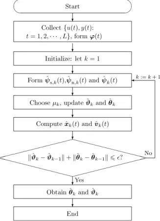
The steps involved in the algorithm in
(31)–(40)
are listed in the following.
1. Collect the input/output data
{
u
(
t
),
y
(
t
)
:
t
=
1
,
2
, . . . ,
L
}
(
L
: the data length), form
ϕ
(
t
)
by
(33).
2. To initialize, let
k
=
1,
ϑ
ˆ
0(
t
)
=
1
n+nd/
p
0,
ˆ
θ
T0(
t
)
=
1
m×(nr)/
p
0,
x
ˆ
0(
t
)
=
1
m×1/
p
0,
v
ˆ
0(
t
)
=
1
m×1/
p
0,
p
0=
10
6.
3. Form
ψ
ˆ
s,k(
t
)
by
(35),
ψ
ˆ
n,k(
t
)
by
(36), and
ψ
ˆ
k(
t
)
by
(34).
4. Choose a large convergence factor
µ
ksatisfying
(40)
and update
ϑ
ˆ
kand
θ
ˆ
kby
(31)
and
(32), respectively.
5. Compute
x
ˆ
k(
t
)
by
(38)
and
v
ˆ
k(
t
)
by
(39).
6. Compute the errors
‖ ˆ
ϑ
k− ˆ
ϑ
k−1‖
and
‖ˆ
θ
k− ˆ
θ
k−1‖
, if
‖ ˆ
ϑ
k− ˆ
ϑ
k−1‖ + ‖ˆ
θ
k− ˆ
θ
k−1‖
⩽
ϵ,
then terminate the procedure and obtain the iteration times
k
and estimates
ϑ
ˆ
kand
θ
ˆ
k; otherwise, increase
k
by 1 and
go to step 3.
The flowchart of computing the parameter estimates
ϑ
ˆ
kand
θ
ˆ
kin the OEMA-HGI algorithm in
(31)–(40)
is shown in
Fig. 1.
Fig. 1. The flowchart for computing the parameter estimates
θ
ˆ
kandϑ
ˆ
kwith finite measurement data.5. Example
Consider the following two-input two-output OEMA system,
y
(
t
)
=
Q
(
z
)
α(
z
)
u
(
t
)
+
D
(
z
)
v
(
t
),
where
y
(
t
)
=
[
y
1(
t
)
y
2(
t
)
]
,
u
(
t
)
=
[
u
1(
t
)
u
2(
t
)
]
,
v
(
t
)
=
[
v
1(
t
)
v
2(
t
)
]
,
α(
z
)
=
1
−
0
.
85
z
−1,
D
(
z
)
=
1
+
0
.
60
z
−1,
Q
(
z
)
=
[
2
.
00
1
.
00
1
.
00
2
.
00
]
z
−1.
In simulation, the inputs
{
u
1(
t
)
}
and
{
u
2(
t
)
}
are taken as two persistent excitation signal sequences with zero mean and
unit variance, and
{
v
1(
t
)
}
and
{
v
2(
t
)
}
as two white noise sequences with zero mean and variances
σ
21
=
σ
22=
0
.
50
2.
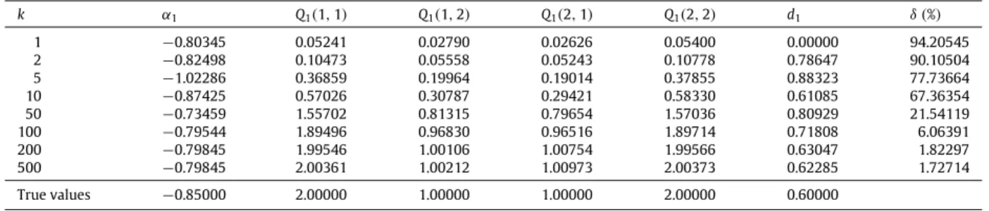
Apply the proposed OEMA-HGI algorithm in
(31)–(40)
to estimate the parameters of this example system, the parameter
estimates and their errors with different data lengths
t
=
L
=
1000, 2000 and 3000 are shown in
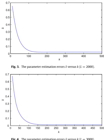
Tables 1–3
and the
parameter estimation errors
δ
:=
‖ ˆ
ϑ
k−
ϑ
‖
2+ ‖ˆ
θ
k
−
θ
‖
2‖
ϑ
‖
2+ ‖
θ
‖
2versus
k
are shown in
Figs. 2–4.
From
Tables 1–3
and
Figs. 2–4, we can draw the following conclusions.
•
The parameter estimation errors given by the OEMA-HGI algorithm become small as the iteration
k
increases.
•
The parameter estimation errors given by the OEMA-HGI algorithm become small with the data length
L
increasing.
•
The OEMA-HGI iterative algorithm can generate more accurate parameter estimates compared with its corresponding
recursive algorithm.
Table 1
The parameter estimates and errors (L
=
1000).k
α
1 Q1(
1,
1)
Q1(
1,
2)
Q1(
2,
1)
Q1(
2,
2)
d1δ (
%)
1−
0.81125 0.04941 0.02860 0.02375 0.05669 0.00000 94.22492 2−
0.83135 0.09821 0.05677 0.04725 0.11259 0.79502 90.19073 5−
1.03317 0.36209 0.19049 0.18321 0.37915 0.86564 77.96435 10−
0.86104 0.55989 0.29573 0.28539 0.58730 0.63319 67.68741 50−
0.95675 1.57436 0.80341 0.79323 1.61044 0.68921 19.78192 100−
0.91679 1.88661 0.94766 0.93989 1.90432 0.75786 7.21823 200−
0.90599 1.98041 0.99147 0.97764 1.99237 0.71810 4.04095 500−
0.90503 1.98794 0.99542 0.98003 2.00003 0.71396 3.86801 True values−
0.85000 2.00000 1.00000 1.00000 2.00000 0.60000 Table 2The parameter estimates and errors (L
=
2000).k
α
1 Q1(
1,
1)
Q1(
1,
2)
Q1(
2,
1)
Q1(
2,
2)
d1δ (
%)
1−
0.80345 0.05241 0.02790 0.02626 0.05400 0.00000 94.20545 2−
0.82498 0.10473 0.05558 0.05243 0.10778 0.78647 90.10504 5−
1.02286 0.36859 0.19964 0.19014 0.37855 0.88323 77.73664 10−
0.87425 0.57026 0.30787 0.29421 0.58330 0.61085 67.36354 50−
0.73459 1.55702 0.81315 0.79654 1.57036 0.80929 21.54119 100−
0.79544 1.89496 0.96830 0.96516 1.89714 0.71808 6.06391 200−
0.79845 1.99546 1.00106 1.00754 1.99566 0.63047 1.82297 500−
0.79845 2.00361 1.00212 1.00973 2.00373 0.62285 1.72714 True values−
0.85000 2.00000 1.00000 1.00000 2.00000 0.60000 Table 3The parameter estimates and errors (L
=
3000).k
α
1 Q1(
1,
1)
Q1(
1,
2)
Q1(
2,
1)
Q1(
2,
2)
d1δ (
%)
1−
0.78828 0.05645 0.02683 0.02704 0.05397 0.00000 94.14136 2−
0.80704 0.11234 0.05341 0.05386 0.10748 0.77324 89.95537 5−
0.98555 0.39079 0.19031 0.18938 0.38153 0.89666 77.33474 10−
0.74582 0.58989 0.28724 0.28696 0.57572 0.76111 67.63875 50−
0.93266 1.69083 0.83691 0.84256 1.66266 0.78092 16.46228 100−
0.90074 1.93359 0.96064 0.97246 1.91098 0.65877 4.31889 200−
0.89054 1.99894 0.99448 1.00848 1.98275 0.59525 1.36572 500−
0.88989 2.00295 0.99659 1.01080 1.98767 0.59066 1.33230 True values−
0.85000 2.00000 1.00000 1.00000 2.00000 0.60000Fig. 2. The parameter estimation errors