Nsubuga, R; Goldstein, M; White, R (2018) Approximate Bayesian Computation and simulation based inference for complex stochastic epidemic models. Statistical science. ISSN 0883-4237
Downloaded from: http://researchonline.lshtm.ac.uk/4646126/ DOI:
Usage Guidelines
Please refer to usage guidelines at http://researchonline.lshtm.ac.uk/policies.html or alterna-tively [email protected].
Approximate Bayesian
Computation and
simulation-based inference for
complex stochastic epidemic
models
∗
Trevelyan J. McKinley, Ian Vernon, Ioannis Andrianakis, Nicky McCreesh, Jeremy E. Oakley, Rebecca N. Nsubuga, Michael Goldstein and Richard G. White
University of Exeter, London School of Hygiene and Tropical Medicine, Durham University, University of Sheffield and MRC/UVRI Research Unit on AIDS
Abstract.Approximate Bayesian Computation (ABC) and other simulation-based inference methods are becoming increasingly used for inference in complex systems, due to their relative ease-of-implementation. We briefly review some of the more popular variants of ABC and their application in epidemiology, before using a real-world model of HIV transmission to illustrate some of challenges when applying ABC methods to high dimen-sional, computationally intensive models. We then discuss an alternative approach—history matching—that aims to address some of these issues, and conclude with a comparison between these different methodologies.
1. INTRODUCTION
Complex mathematical models can provide important insights into the be-haviour of dynamic epidemiological systems. However, to understand how well the model represents reality, and therefore how useful the model is for inference regarding the actual system under study, it is necessary to fit it to observed data. This task can be challenging, partly due to the complexity of the model itself, but also because there is often a paucity of available data.
Common features of models used to study real-world epidemiological processes are that they are large-scale, dynamic, non-linear and auto-correlated. Further-more, information such as infection times are almost impossible to measure or
College of Engineering, Mathematics and Physical Sciences, University of Exeter, Penryn, UK.(e-mail: [email protected]) London School of Hygiene and Tropical Medicine, Keppel Street, London, UK. Department of Mathematical Sciences, Durham University, Durham, UK. School of Health and Related Research, University of Sheffield, Sheffield, UK. MRC/UVRI Research Unit on AIDS, Entebbe, Uganda.
∗
This work was supported by a Medical Research Council (UK) grant on Model Calibration (MR/J005088/1) (http://www.mrc.ac.uk/).
record, and so the observed data often correspond to proxies such as medical re-ports, test results and mortality rates, and even these are frequently incomplete. These challenges have driven the development of a suite of statistical method-ologies for model fitting, the most widespread of which are based around the use of a likelihood function. Here we focus on Bayesian methods, where we wish to estimate the posterior distribution for the parameters (θ), given the data (y), which can be written as:
(1) π(θ |y)∝π(y|θ)π(θ),
whereπ(y|θ) is the likelihood function andπ(θ) is the prior distribution (rep-resenting our beliefs in the values of the parameters in the absence of data). Usually the normalising constant is analytically intractable, requiring the use of numerical methods to generate empirical estimates ofπ(θ|y).
In many cases the likelihood is also intractable, due to the presence of hid-den variables (or missing data), and some form of imputation method is usually required in which the missing information is inferred. Data-augmentation (DA) methods (e.g.Gibson and Renshaw,1998,O’Neill and Roberts,1999,Jewell et al.,
2009) provide a flexible and powerful framework for inference, where the parame-ter space is augmented to include the hidden variables (x). The marginal posterior distribution of interest is then given by
(2) π(θ|y) =
Z
X
π(θ,x|y)dx,
where X corresponds to the (multidimensional) parameter space for the hidden
variables. The integrand in (2) can be written as
(3) π(θ,x|y)∝π(y,x|θ)π(θ),
where the joint likelihood function based on the observed data and the hidden variables,π(y,x|θ), is now tractable. If joint samples fromπ(θ,x|y) can then be produced (using numerical sampling algorithms such as Markov chain Monte
Carlo—MCMC), then the integral in (2) is straightforward to evaluate
numeri-cally. The uncertainties due to the hidden variables are intrinsically incorporated into the resulting marginal posterior distribution. Despite their flexibility, these methods can quickly become computationally infeasible as the number of hidden variables, and the size and complexity of the system increases; not only because the additional variables must be stored, but also because designing and imple-menting efficient update schemes for the augmented variables in high dimensions can be very challenging (both methodologically and computationally).
An alternative approach is to consider that the marginal posterior (2) can also be written as (4) π(θ|y)∝ Z X π(y,x|θ)dx π(θ),
and the integral in (4) can be approximated using importance sampling as
(5) πˆ(y|θ) = 1 n n X i=1 π(y,xi |θ) qX(xi |θ) ,
where xi ∼ qX(· |θ) and qX(· |θ) is a proposal distribution for the hidden
variables x. Some powerful theoretical results follow from this estimator.
In-deed, Beaumont [2003] proved that using the estimator (5) in an MCMC
algo-rithm of the form given in Algoalgo-rithm 1.1a (with (5) replacing ˆπ(y|θ)), gave exact posterior samples in probability. This result was later generalised by An-drieu and Roberts [2009], who showed that this holds for any non-negative un-biased estimator of π(y|θ). In practice, the key challenge is finding efficient proposal distributions,qX(· |θ), for the hidden variables, which can be difficult for complex non-linear models [see e.g. Andrieu et al., 2010, McKinley et al.,
2014,Drovandi et al.,2016].
1.1 Direct simulation from the underlying model
In certain situations, it may be possible to simulate outputs directly from an underlying statistical model, which can then be mapped to the observed data in an appropriate manner. In this case equation (4) becomes
(6) π(θ|y)∝ Z Z π(y|z,θ)π(z|θ)dz π(θ),
whereπ(z|θ) is the likelihood function for a single realisation of the underlying process, z, and π(y|z,θ) is a probabilistic mapping between the realisation z
and the observed datay. (Z corresponds to the space of all possible realisations ofz.) We can then write equation (5) as:
(7) πˆ(y|θ) = 1 n n X i=1 π(y|zi,θ),
wherezi∼π(· |θ) corresponds to a single simulation from the underlying model. In the special case that we require exact matching between the simulated data and the observed data, then
(8) π(y|zi,θ) =
(
1 ifzi=y,
0 otherwise.
In other cases we could define the mapping between zi and y to have a
spe-cific probabilistic form (for example, if the observed data were derived from an imperfect diagnostic test). From now on we will focus on systems that can be written in the form described by (6). (Note that there are also promising
meth-ods that involve recoding or reparameterising the simulation model (e.g. Neal,
2010,McKinley et al.,2014,Kypraios et al.,2016). However, these approaches are not feasible for all models, and can be difficult to scale to very complex systems, so here we focus on methods that simulate directly from the underlying model.) These ideas, coupled with the fact that it is often far easier to code a simula-tion model than reconstruct a likelihood funcsimula-tion based around a large number of hidden variables, have facilitated the development of various ‘simulation-based’ methods for inference, where calculation of the likelihood is replaced by an esti-mate derived from simulations from the underlying model, an idea that goes back at least as far as Diggle and Gratton [1984] and Rubin [1984]. The key bottle-neck in the implementation of these methods is that even for small-scale systems, the probability of generating simulations that match all observed data points
exactly is often very small. This often precludes direct implementation of these approaches, and instead motivated the development of a suite of techniques now
known colloquially as Approximate Bayesian Computation (ABC) [e.g. Tavar´e
et al., 1997]. In recent years these techniques have exploded in popularity, since these ideas can be readily incorporated into existing numerical algorithms, such as rejection sampling [e.g.Tavar´e et al.,1997,Beaumont et al.,2002]; MCMC [e.g.
Marjoram et al.,2003,Ratmann et al.,2009, Wood, 2010]; or sequential Monte Carlo [SMC] [e.g. Sisson et al., 2007, Toni et al., 2009, Beaumont et al., 2009,
Del Moral et al.,2011,Drovandi and Pettitt,2011,Lenormand et al.,2013]. Due to their relative ease-of-implementation, simulation-based methods are being in-creasingly adopted in stochastic epidemic modelling (e.g. O’Neill et al., 2000,
Toni et al., 2009, McKinley et al., 2009, 2014, Neal, 2010, Conlan et al., 2012,
Brooks Pollock et al.,2014,Kypraios et al.,2016).
Good reviews of ABC can be found in Csill´ery et al. [2010] and Beaumont
[2010], and a more recent and technical review can be found in Marin et al.
[2012]. In many applications, vanilla rejection sampling approaches are hard
to implement efficiently, and so most ABC routines in the literature are based around either MCMC or SMC methods; two popular examples are shown in
Al-gorithms 1.1a and 1.1b. We assume the reader is familiar with both SMC and
MCMC methods [see e.g. Marjoram et al.,2003,Toni et al.,2009]. A recent tu-torial for implementing ABC-MCMC methods for temporal stochastic epidemic
models can be found in Kypraios et al. [2016]. The fundamental challenge for
implementation of ABC is that in many circumstances the probability of get-ting an exact match between the simulations and the data is vanishingly small, and there have been myriad innovations to try to alleviate this problem. Here we briefly introduce some of the more common ABC-type approaches, before fo-cusing on key challenges when applying these methods to high-dimensional and computationally intensive models.
2. ‘CLASSIC’ ABC
Instead of requiring the simulations to match the data exactly, a distance metric,ρ(·,·), can be introduced, and thus (7) can be approximated by:
(9) πˆ(y|θ) = 1 n n X i=1 1(ρ(y,zi)< ),
with defining some tolerance for matching. Using the estimator (9) as an
es-timate of the likelihood in standard numerical procedures will produce samples from theapproximateposteriorπ(θ|ρ(y,·)< ). Generally speaking, the metric is set-up such that ρ(y,zi)→0 as zi→y, and hence as→0 the approximate posterior will tend to the true posterior, but at a greater computational cost.
2.1 The impact of the tolerance
A key consideration is fixing (or reducing) the tolerance levels to be as small as possible (in order to minimise information loss in the approximate posterior), whilst retaining a reasonable acceptance rate. SMC methods are well-suited to the ABC framework, since they allow initial generations to use less restrictive tolerances than subsequent generations, which often makes them more efficient at exploring the parameter space than ABC-MCMC, provided a good set of initial
A1. Initialise the tolerance, the number of iterations niter.
A2. Sample an initial set of parametersθ(0)∼π(θ). A3. Generatendata setsz(0)i ∼π · |θ
(0)and calculate ˆ π y|z(0)i = (1/n)Pn i=11 ρ y,z(0)i < . A4. If ˆπ y|z(0)i = 0 go to stepA2. A5. Set iteration indicatorj= 1.
A6. Sample a candidate valueθ0∼Q ·|θ(j)from some Markov transition kernelQ(·). A7. Generatendata setsz0
i∼π(· |θ0) and calculate ˆ π(y|z0) = (1/n)Pn i=11(ρ(y,z 0 i)< ).
A8. Setθ(j)=θ0and ˆπ y|z(j)= ˆπ(y |z0) with probability α = min 1, ˆπ(y|z 0) ˆ π(y|z(j−1))× π(θ0) π(θ(j−1))× Q θ(j−1)|θ0 Q(θ0|θ(j−1)) ! ,
else setθ(j)=θ(j−1)and ˆ
π y|z(j)= ˆπ y|z(j−1).
A9. Ifj < niter, incrementj=j+ 1 and go to stepA6.
B1. Set the number of generationsT, and the number of particlesnpart.
B2. Initialise the tolerances1, . . . , T. Set population
indicatort= 1.
B3. Set particle indicatorj= 1.
B4. Ift= 1, sampleθ00independently fromπ(θ). If t >1, sampleθ0from the previous population {θt−1}with weights{Wt−1}, and perturb the particle toθ00∼Qt(· |θ0) according to a Markov
transition kernelQt(·).
B5. Ifπ(θ00) = 0, return toB4. B6. Generatendata setsz00
i∼π(· |θ00), and calculate ˆ π(y|z00) = (1/n)Pn i=11(ρ(y,z 00 i)< t). B7. If ˆπ(y|z00) = 0, then go toB4. B8. Setθ(tj)=θ00and Wt(j)= ˆ π(y|z00) ift= 1, ˆ π(y|z00)π θ(tj) Pnpart j=1 W (j) t−1Qt θ(tj)|θ(tj) −1 ift >1.
B9. Ifj < npart, incrementj=j+ 1 and go to stepB4.
B10. Normalise the weights so thatPnpart
j=1 W
(j)
t = 1.
B11. Ift < T, incrementt=t+ 1 and go toB3.
Algorithm 1.1: The (a) ABC-MCMC algorithm of Marjoram et al. [2003]
(left-panel) and the (b) ABC-SMC algorithm ofToni et al.[2009] (right-panel).
particles can be found [see e.g.Toni et al.,2009,McKinley et al.,2009]. Adaptive schemes are often used [Beaumont et al.,2009,Del Moral et al., 2011,Drovandi and Pettitt,2011,Lenormand et al.,2013], in which the choice of tolerance at each generation is determined as a function of the simulated metric distances at the previous generation (seeSilk et al.,2012 for some critique of these approaches).
ABC-MCMC methods tend to use a fixed tolerance for the entire chain, with
a few notable exceptions: for example Ratmann et al. [2007] use a tempering
method to reduce the tolerance during the burn-in phase, before fixing the tol-erance to collect the final samples, and Bortot et al. [2007] introduce a data-augmentation approach, in which they place a shrinkage pseudo-prior on the tolerance and estimate this as part of the model fitting.
2.2 Matching to multiple outputs
Acceptance rates are affected further when matching to multiple outputs. Here there are two main options: the first, the so-called intersection approach, sets
a separate distance metric around each of the K outputs, each with its own
tolerance. A simulation is then accepted if: (10)
K Y
k=1
1(ρk(y,z)< k) = 1,
wherez corresponds to the simulated data. The simulation must therefore match
each output simultaneously in order to be accepted. An alternative is to create
a single metric,ρ∗(·,·), and accept a simulation if: (11) 1(ρ∗(y,z)< ) = 1,
whereρ∗(y,z) =f(ρ1(y,z), . . . , ρK(y,z)), andf(·) is some function of the K outputs [e.g.Conlan et al.,2012]. This is termed aunionmetric (see alsoRatmann et al.,2014).
The trade-off between the two choices varies according to the particular system being modelled, but heuristically one can think of the union metric as smoothing out some of the patterns in the data—i.e. the models are allowed to fit certain outputs less well than others, provided that the overall fit is reasonable. Com-bining metrics in a sensible manner is sometimes challenging, especially if they are defined on different scales [see e.g. Conlan et al., 2012]. Union metrics can sometimes lead to simulations being regularly accepted when they do not fit cer-tain outputs very well at all, whereas intersection metrics can penalise misfitting simulations more, but at a cost of reduced acceptance rates. In the case of ABC we expect the probability of rejecting a simulation to scale withK (although of course the exact relationship is harder to quantify, since some of the metrics may be correlated).
2.3 The use of summary statistics
Based on the previous discussion, if the dimensionality of the observed data is large then it can be challenging to design a computationally efficient algorithm with minimal information loss in the approximate posterior. In a handful of cases,
it may be possible to reduce the data to a set of lower-dimensional sufficient
statistics, that contain the same amount of information as the full data. More often that not, sufficient statistics are unknown (or are equal to the data), and so often a set of lower-dimensional summary measures, S1(y), . . . , SL(y), are used
in their place (where L < K). The key questions are then: how well do the
summary statistics capture the information in the data, and how do any biases introduced manifest in any inferences that we make from the model? Increasing
research effort has been placed into deriving approximately sufficient summary
measures [e.g.Joyce and Marjoram,2008,Nunes and Balding,2010,Barnes et al.,
2012, Fearnhead and Prangle,2012,Ratmann et al.,2014]. The use of summary statistics can also be extended toindirect inference methods, where the auxiliary models describe the distributions of the summary statistics (see Section2.7).
2.4 Increasing the number of replicates (n >1)
Interestingly, theoretical convergence of Algorithms 1.1a and1.1b do not de-pend on the number of simulations, n, used in the estimator (9) [Andrieu and Roberts,2009,Del Moral et al.,2011]. For more general classes of pseudo-marginal algorithms it has been shown that increasingn can improve the efficiency of the algorithms by reducing the variance of the estimator (5) [see e.g.Pitt et al.,2012,
Sherlock et al., 2015, Doucet et al., 2015]. In the specific case of ABC-MCMC
with uniform matching, Bornn et al. [2017] show that setting n = 1 results in
run times that are at most a factor of 2 away from the optimum choice (obtained for some n >1). However, their results also make the assumption that simula-tion run times are approximately constant, which is often not true for epidemic systems, where run times for individual simulations can often vary greatly even for fixed parameter inputs. Also, in the case of ABC-MCMC and more general
pseudo-marginal algorithms, chains using low values of n can often get ‘stuck’
and fail to mix practically at all [see e.g. McKinley et al., 2009, Andrieu and Roberts,2009]. Mixing can generally be improved by increasing the tolerance(s),
but at the cost of further information loss in the approximate posterior. Under the same assumptions as above,Bornn et al.[2017] show that for a simple
rejec-tion sampling ABC algorithm, n = 1 is indeed optimal. In practice ABC-SMC
samplers, such as described in Algorithm 1.1b seem to perform better for low
n[see e.g.McKinley et al.,2009], and it is for this reason that we choose to use ABC-SMC instead of ABC-MCMC for tackling the model in this paper.
Another option to alleviate the mixing issues in pseudo-marginal MCMC algo-rithms for low nis to refresh the ˆπ(y|θ) estimates for both the candidate and current parameters at each iteration of the chain [see e.g. O’Neill et al., 2000,
Andrieu and Roberts, 2009, McKinley et al., 2014]. This exhibits substantially better mixing, at the cost of producing biased samples, with the bias decreasing
as n → ∞. It also doubles the number of simulations required per iteration of
the chain, though this is often mediated by requiring shorter chains due to the improvement in mixing.
2.5 Interpretation of ABC posterior
The term ABC derives from the fact that these methods were originally devel-oped to obtain an approximation to the ‘true’ posterior (Tavar´e et al.,1997). Wilkin-son [2013] showed that in certain circumstances, for a fixed metric and (final)
tolerance, ABC can be interpreted as giving the exact posterior under the
as-sumption of model error. For example, if ρ(·,·) is based on Euclidean distances,
then up to some normalising constant, (9) corresponds to assuming uniform
er-ror around the observed data y (these normalising constants then cancel in the
accept-reject steps of Algorithms 1.1a and b).
Wilkinson[2013] cites two possibilites for the interpretation of the error term: observation error or model discrepancy. The former is generally well understood, and it is often possible to either build this directly into the simulation code, or define this in terms of a probabilistic function mapping the hidden states to the observed data. The idea of model discrepancy (MD) is less familiar, and more difficult to define, but relates to the disparity between the model and reality. It has been argued to be an important source of uncertainty that should be incorporated into calibration routines to prevent overinterpretation due to the
choice/assumptions of the model, and hence increase robustness [e.g. Goldstein
and Rougier,2009,Oakley and Youngman,2015]. When viewed in this way, ABC ceases to be approximate. In practice, for this interpretation to be meaningful re-quires that the form and magnitude of MD is considered in advance and specified in epidemiologically relevant terms (see e.g. Section 2.6). When we discuss ‘clas-sic’ ABC in this paper, we do so in its original paradigm, that of an approximation to the posterior in the absence of MD.
Another important contribution is given inFearnhead and Prangle [2012], in
which they reframe ABC inference in terms of a set of desired properties
(de-fined as accuracy and calibration), and provide methods for selecting summary
statistics to optimise these desired characteristics.
2.6 Generalised ABC and post-processing
Beaumont et al. [2002] suggested improving the posterior approximation by
post-processing the final set of parameters; reweighting each according to the dis-tance between the simulated outputs and the data using localised linear-regression (see alsoBlum and Fran¸cois,2010). An alternative is to choose some non-uniform
discrepancy distribution for use directly within the ABC estimate of the likeli-hood. Hence (9) becomes:
(12) πˆ(y|θ) = 1 n n X i=1 π(y|zi, ),
where >0 now defines some variance controlling the discrepancy between the
simulated and observed data sets.Wilkinson [2014] terms this generalised ABC
(GABC). A natural choice of discrepancy distribution is one that has a single mode, centred around the observed data, such that π(y|zi, ) → 0 as the
dis-tance between y and zi increases. As an example, we could place independent
Gaussian distributions with variancearound each data point, or even used
dif-ferent variances for difdif-ferent data points. (Note also that (12) also includes the uniform discrepancy distribution discussed earlier as a special case.) The lack of hard-bound on the discrepancy distribution removes the problem of ‘matching’,
but at the potential cost of (12) having a high Monte Carlo variance unless a
large number of replicates is used. This could lead to mixing issues in ABC-MCMC and particle degradation in ABC-SMC. A truncated, but non-uniform, error term could alleviate the high uncertainty when simulating in the tails of the discrepancy kernel (see also the ideas inBortot et al.,2007andBeaumont et al.,
2002).
2.7 Indirect inference
There are also a series of approaches that are akin to the methods ofindirect inference [Gouri´eroux et al.,1993], whereby an auxiliary model is introduced to describe the distribution of the data, and inference is based on comparison of the parameters of the auxiliary model as estimated through repeated simulations
from the model-of-interest [e.g. Wood, 2010, Drovandi et al., 2011, Ratmann
et al.,2014]. The synthetic likelihood approach of Wood[2010] assumes a para-metric form (e.g. multivariate normal) for the distribution of outputs arising from repeated model simulations. The parameters of this auxiliary model are estimated from the simulations, and a synthetic likelihood can be constructed by estimating the likelihood that the observed data come from the auxiliary model. A huge ad-vantage of this method is that there is no need to choose tolerance levels for the matching, though a suitable auxiliary model must be found (which is sometimes challenging), and replicate simulations per parameter set are necessary.
An insightful paper by Drovandi et al. [2014], showed that classical ABC and the synthetic likelihood approaches are both special cases of a more general class of models, which they call Bayesian indirect likelihood (BIL) models. They show that in general convergence of the synthetic likelihood approach to the true pos-terior is not guaranteed, however the method often performs well if the auxiliary model is flexible enough to match the simulations to the data well in the region of non-negligible posterior mass.
3. CHALLENGES FOR COMPUTATIONALLY INTENSIVE MODELS
In the previous section we briefly reviewed various recent advances in simulation-based inference for statistical models. There are many possible choices of ap-proach, with trade-offs in terms of computational complexity, accuracy, bias,
interpretation and ease-of-implementation. The ability to plug a simulation al-gorithm into existing routines have made ABC-type methods attractive as a po-tential tool for statistical inference in large-scale, complex systems, such as those frequently studied in epidemiology (see also Ionides et al., 2006,2011, 2015 for frequentist approaches). In addition it is often straightforward to parallelise the simulations.
Nonetheless, most methodological research has focused on the development of ideas and theories applied to relatively small scale models or data sets, and even some of these simpler examples can take between several hundred thousand
model runs to many millions [e.g. Kypraios et al., 2016]. In our opinion, one
of the major current challenges in the field is how to perform robust inference when the simulation models are highly computationally intensive; precluding the running of very large numbers of simulations. These systems often go hand-in-hand with high-dimensional input (parameter) and output (data) spaces, and in this paper we illustrate some of these challenges using a complex, large-scale, high-dimensional model of HIV transmission. This model, called Mukwano, is an individual-based stochastic micro-simulation model, that simulates (amongst other things): heterosexual sexual partnerships, sexual activity, HIV transmission and life histories (including births and deaths). Different versions of the model exist, but the version studied here has 22 input parameters, and 18 outputs.
For brevity we refer the reader toAndrianakis et al.[2015] for full details of the model, but briefly the model simulates heterosexual sexual partnerships (partner-ship formation, dissolution, and concurrency) and HIV transmission, alongside demographic events such as births and deaths in a population of individuals. The data come from a long-term (25+ years) longitudinal study of an open cohort of ≈18,000 individuals in rural Uganda. We used informative uniform priors for the
22 inputs, and full details of the model and priors can be found in Andrianakis
et al. [2015].
The model has an average run time of ≈5–10 mins per simulation (in the
well-supported region—it can be far longer [>3 hours] in some areas of poor support). Based on the discussions in earlier sections, and our own experience, it was decided that an ABC-SMC algorithm, using a single simulation per particle (n= 1) would be a sensible choice of routine to try to tackle this problem. Some initial tests using GABC with normally distributed discrepancy terms resulted in extremely high Monte Carlo errors for the GABC likelihood estimate in parts of the space where the model fit was poor. As such we instead used a uniform error term and implemented an intersection approach in which all 18 outputs were matched simultaneously. We set a non-zero minimum bound for the tolerance, relating to roughly twice the observation standard deviation for each output used inAndrianakis et al. [2015].
We implemented the ABC-SMC routine ofToni et al.[2009] (Algorithm1.1b),
using the optimal localised multivariate kernel approach of Filippi et al. [2013]. In order for ABC to work well, there must be a large enough number of particles located in areas of high posterior support, and so we generated an initial set of 22,000 particles uniformly from the prior distribution. Here we choose to match to 18 outputs simultaneously, which requires 18 tolerances defined on different scales. We chose initial tolerance values to be the 50th percentile of the simulated metric distances for each of the 18 outputs, and chose tolerances at generationt+1
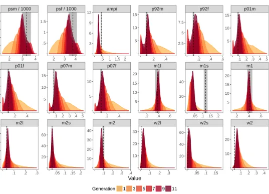
m2l m2s m2 w2l w2s w2 p01f p07m p07f m1l m1s m1 psm / 1000 psf / 1000 ampi p92m p92f p01m .1 .2 .3 .05 .1 .15 .2 .1 .2 .3 .4 .1 .2 .3 .05 .1 .15 .1 .2 .3 .4 .2 .4 .1 .2 .3 .4 .5 .2 .4 .2 .4 .6 .05 .1 .15 .2 .2 .4 .6 2 3 4 2 3 4 .5 1 1.5 2 .2 .4 .2 .4 .6 .1 .2 .3 .4 .5 5 10 15 5 10 15 20 10 20 2.5 5 7.5 20 40 20 40 60 5 10 15 5 10 15 20 10 20 30 3 6 9 12 5 10 10 20 30 40 .5 1 1.5 5 10 15 20 40 60 .5 1 1.5 2 2.5 2.5 5 7.5 10 12.5 10 20 30 40 Value Density Generation 1 3 5 7 9 11
Fig 1: Model fits for 11 generations of ABC. These show the marginal predictive distributions for the model outputs conditional on the set of ABC particles at different generations of ABC. For brevity we only show generations 1, 3, 5, 7, 9 and 11 here. The dotted lines denote the data and the target regions are shown in grey.
using a simple bisection method (detailed inSupplement A), where the proportion
of generation t particles that would be accepted using the new tolerances was
approximately pτ = 0.5. (We note that this method allows for semi-automatic
non-uniform adjustments of the tolerances at each generation of ABC, and can also be applied to outputs that are defined on different scales.)
The results for 11 generations of ABC-SMC are shown in Figure 1, which
shows some interesting behaviour. For most outputs there is a steady
conver-gence towards the observed data. However, for one output in particular (m1s),
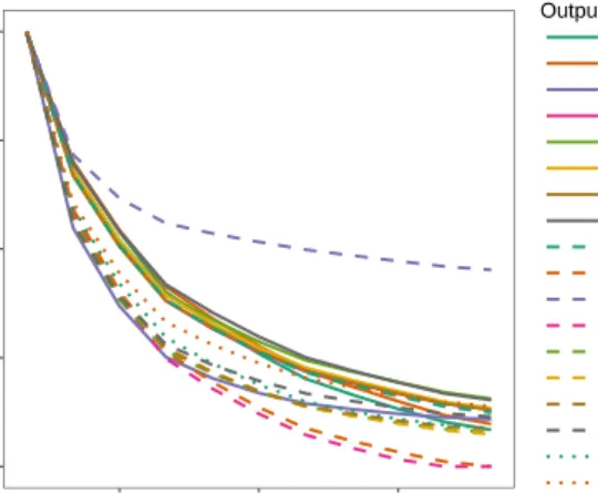
even after 11 generations of ABC the simulated outputs are far lower than the observed data (see also theampi output). Figure2shows the relative tolerances across generations, rescaled such that a value of one corresponds to the initial tolerance, and zero to the target (observation) tolerance. The algorithm should stop when each line crosses zero. The blue line relating to them1s output seems to be asymptoting at a level far higher than we require, and indeed for many of the others the rate-of-change of tolerance values between the generations is also slowing. Although the aim is to generate an acceptance rate of around 0.5 for each generation, in the later generations the actual value is much smaller than this (Table1). At this point the final generation took almost 2 days to run on a high-performance cluster.
These anticipated challenges for ABC in higher dimensions present a difficult set of choices for the standard ABC paradigm: do we continue to run the algorithm as before, considering the decreasing convergence rate; do we change criteria in the
0.00 0.25 0.50 0.75 1.00 3 6 9 Generation Relativ e toler ance Output psm psf ampi p92m p92f p01m p01f p07m p07f m1l m1s m1 m2l m2s m2 w2l w2s w2
Fig 2: Relative tolerance evolution (right panel) for 11 generations of ABC-SMC fitted to Mukwano. (Note that arelative tolerance of 1 corresponds to the initial
tolerance value at the first generation of ABC-SMC, and a relative tolerance of
0 corresponds to the target tolerance defined by the observation error, as shown by the grey regions in Figures1 and 3.)
Generation 1 2 3 4 5 6 7 8 9 10 11 Total
Acc. rate 0.78 0.64 0.59 0.49 0.44 0.37 0.3 0.27 0.2 0.16 0.15
Number sims. 28,363 34,407 37,377 45,062 49,816 58,989 72,325 82,236 109,651 139,329 142,764 800,319
Table 1
Acceptance rates for ABC-SMC
algorithm, perhaps choosing smaller tolerance thresholds at the cost of decreasing acceptance rates further; do we change metric; or do we stop the algorithm? On the one hand there seems to be convergence towards the data, so one could continue with the ABC. On the other hand the rate of convergence is slowing, and the number of simulations required at each generation is increasing, to the point that we may begin to question the logic of continuing. If the tolerances asymptote to a level that is far away from the data, then the key question is: can the model fit the data adequately, or have we simply not explored the parameter space sufficiently? Sometimes the trade-offs in accuracy required to get ABC algorithms to fit in a computationally feasible manner can be large, and can lead to situations in which the current ‘best-fit’ from the ABC algorithm is sufficiently poor that we are unable to make useful inferences about the system.
3.1 Emulation
A advance for approximating outputs when a simulation model is computa-tionally expensive is to appeal to the use of anemulator [e.g.Sacks et al.,1989]. This is a statistical representation of the simulation model that can be used as a surrogate in simulation-intensive routines. Typically, the complex model is run at a series of ‘design’ points, and the emulator is trained on the simulated outputs at each of these points. Once trained, the emulator can be used to predict the outputs from the complex model (as well as to provide measures of uncertainty in the predictions) very quickly.
emulators within ABC. Henderson et al. [2009], Jandarov et al. [2014], Wilkin-son[2014], Meeds and Welling [2014] and Cameron et al.[2015] each implement MCMC algorithms where the true likelihood is replaced by that derived from an emulator. Important differences between the methods lie in how the emulator is trained.Henderson et al. [2009] use a fixed set of design points (chosen to cover the input space), andJandarov et al. [2014] use a grid design. These are feasible because the input and output spaces are low-dimensional, but would be chal-lenging in high dimensions, since enough points would be required to produce a sufficiently accurate emulator.Meeds and Welling[2014] train the emulator as the MCMC progresses, choosing new design points based on local moves around the current point of the chain.Jabot et al. [2014] embed the emulator in both rejec-tion and SMC samplers, using initial design points sampled from the prior. ABC steps are then run using the emulator as a surrogate, and new training points
chosen at each generation based on the current set of particles. Cameron et al.
[2015] use functional regression to emulate a microsimulation model of malaria infection, which they use to generate an approximate posterior through MCMC. These approaches look promising, but require an emulator that is sufficiently accurate to represent the complex model across the input space, which in turn requires careful design of training points. In the next section we discuss an al-ternative methodology that is specifically designed to rigorously and efficiently explore high dimensional input spaces to reject areas where the model fits are poor.
3.2 History matching
History Matching (HM) is a technique developed in the Bayesian computer model literature for finding acceptable inputs to expensive complex models that have high dimensional input and output spaces [Craig et al., 1997]. It has been successfully employed across a range of scientific disciplines, both for deterministic and stochastic models (see Vernon et al. [2010,2014], Andrianakis et al. [2015] and references therein). While there may appear to be superficial similarities between HM and various versions of ABC, the techniques are distinct both in terms of their goal and their implementation. HM is not an inferential procedure, but instead seeks to identify the regions of input space that produce acceptable matches between model and data, where ‘acceptable’ is defined via an underlying statistical model that incorporates a careful consideration of major uncertainties: observational errors, model discrepancy and others (e.g. stochasticity).
It proceeds by cutting out regions of the input space in iterations or waves, us-ingimplausibility measures. In each wavet, we design a set of model runs over the current input space Θt. The set of outputs is denotedK ={1, . . . , K}. Emulators
(such as Gaussian processes) are constructed only over Θt to mimic informative
outputs of the model (deterministic case) or summaries of outputs (stochastic case), denoted fk(θ), providing estimates of the expected values and variances, E(fk(θ)) and Var(fk(θ)) respectively. At wave t it is only necessary to choose a set of outputsk∈ Ktthan can both be emulated sufficiently accurately, and that are informative: usually this set increases in size at each wave. An implausibility measure can then be constructed for each emulated output fk(θ), k ∈ Kt (more
advanced implausibility measures are available):
(13) Ik2(θ) = (E(fk(θ))−yk)
2
Var(fk(θ)) + Var(k) + Var(ek)
.
Here yk is the observed data, and Var(k) and Var(ek) are the variances due to model discrepancy and observation error respectively. The structure of Ik(θ) is derived from an underlying statistical model [Vernon et al.,2010], which dictates how to combine the different sources of uncertainty. Because the specified uncer-tainties are meaningful, unlike the tolerances in standard ABC, the implausibility is also now on a meaningful scale, and we can apply cutoffs onIk(θ) directly (mo-tivated by Pukelsheim’s 3σ rule [Pukelsheim,1994]) to remove implausible parts of the input space ifIk(θ)> c (where often c = 3). Large amounts of the input
space Θt can often be removed based on a single (or a small combination of)
output(s), to define a reduced space Θt+1. Further waves are performed unless
a) the emulator variances Var(fk(θ)) for all outputs of interest are now small in comparison to the other sources of uncertainty Var(k) + Var(ek), or b) the entire input space has been deemed implausible.
Why is this a useful approach?HM works well in high dimension for several reasons [Vernon et al.,2010]. It provides a fast, meaningful decision, based on a subset of outputs, as to whether an input point is implausible that is independent of the rest of the input space, and hence can quickly discard vast regions of input space without modelling the whole set of outputs. Note that these regions will most likely contain extremely low posterior probability, hence, although HM does not seek a Bayesian posterior, it is a very useful precursor if one subsequently wishes to do so. Critically, at each wave the emulator accuracy is expected to im-prove, and structured emulators involving dimensional reduction can be designed to exploit this. Often an individual output may strongly depend only on a small subset of ‘active’ inputs [e.g. Vernon et al., 2010], and hence the implausibility structure allows us to break a high dimensional problem into a series of lower dimensional ones. There may also be several outputs that are difficult to emu-late in early waves (perhaps because of their erratic behaviour in uninteresting parts of the input space) but simple to emulate in later waves in smaller, more realistic input regions. HM thus allows the sequential incorporation of outputs of increasing complexity.
The differences between HM and ABC: at each wave of HM, all the em-ulators and implausibility cuts from previous waves are also used. Hence, unlike most ABC implementations, HM ‘remembers’ regions of space that were previ-ously deemed implausible. This is vital in high dimensions to avoid unnecessarily retesting many input locations known to be unacceptable. ABC usually seeks to approximate a Bayesian inference calculation, using ever decreasing tolerances that can cause computational inefficiencies. However, HM is not an inferential procedure, nor is it ‘approximate’, and uses tolerances that are derived from a well defined statistical model that incorporates realistic assessments of uncer-tainty that are usually elicited from subject matter experts or by performing simple alternative experiments on the model [Goldstein et al., 2013]. They are hence interpretable, can be substantial, and are not reduced to arbitrarily small sizes, and can alleviate these computational inefficiencies. The statistical model also facilitates the incorporation of additional uncertainties e.g. from the emulator
(while exploiting their independence) and the direct use of implausibility, lead-ing to a more efficient parameter search. HM has natural stopplead-ing criteria, since either the entire space will be ruled as implausible, implying that the complex model is deficient, or the emulators will achieve sufficient accuracy to determine the acceptable set of inputs. While one can mimic certain parts of a basic HM analysis using ABC [Holden et al.,2016], it is hard to justify this from the ABC paradigm alone, and it would arguably lead to an analysis that is not ‘ABC’ in nature. (An interesting variation of HM is given inWilkinson,2014, in which HM is used to match to the GABC log-likelihood. Once trained the emulator is then used directly in ABC.)
In Andrianakis et al. [2015], a history matching approach was applied to the
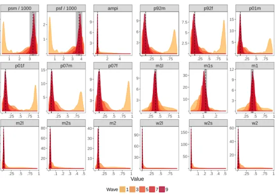
Mukwano model described previously. The model fits are shown in Figure 3,
and required around 355,000 simulation runs (less than half the number of runs
required for 11 generations of ABC). Clearly the model is capable of producing
fits that are close to the observed data, but the non-implausible region is only a tiny proportion (10−11) of the original space.
As a comparison against the ABC-SMC algorithm, we have also calculated the acceptance rates for the final wave of history matching (Table 2). These results show how many simulations from the wave 9 design points would have been accepted using the generation 11 tolerances from the ABC-SMC run, and also how many would have been accepted according to the target tolerance that we are aiming for. We have produced acceptance rates according to simulated mean outputs (averaged across multiple replicates per design point), in addition to a replicate-specific estimate (making the simplifying assumption that all replicates from all design points are independent). We can see that using the generation 11 tolerances we would have had an acceptance rate of 0.48 (mean) and 0.41
(replicate), compared to a value of 0.15 for the ABC-SMC (Table1).
The HM procedure produces high acceptance rates for each output considered on its own, but the curse-of-dimensionality is still clear when trying to match all outputs simultaneously. In fact none of the simulations match all outputs simul-taneously at the target tolerance. Nonetheless, we note that the target tolerances for some of the outputs were small, and so we are happy that we have outputs that are relatively close to these targets. In addition, provided the HM has been performed carefully, if there is a region where all outputs can match simultane-ously (in terms of realisations) then this region should be contained in the current non-implausible region.
One extension to the approach described here is to generate multivariate im-plausibilities. This has been discussed inVernon et al.[2010] in the deterministic model case, but the same framework could be used in the stochastic case provided that we can specify a suitable joint multivariate structure between the simulator outputs. However, these have not been developed yet. Without this, it is simpler to use univariate criteria, and to impose cutoffs on the maximum implausibility to identify joint matches (indeed we view it as a strength of history matching that we can carry out such a combined univariate analysis).
Although HM does not produce an approximate posterior in the same sense as ABC, it is possible to view the marginal densities of non-implausible points
(known as depth plots). We have included these as Supplement B. One must
m2l m2s m2 w2l w2s w2 p01f p07m p07f m1l m1s m1 psm / 1000 psf / 1000 ampi p92m p92f p01m .25 .5 .75 1 .1 .2 .3 .4 .5 .25 .5 .75 1 .25 .5 .75 .1 .2 .3 .4 .5 .25 .5 .75 1 .25 .5 .75 1 .25 .5 .75 .25 .5 .75 1 .25 .5 .75 1 .1 .2 .25 .5 .75 1 1 2 3 1 2 3 4 2 4 .25 .5 .75 .25 .5 .75 1 .25 .5 .75 5 10 15 3 6 9 12 20 40 60 2.5 5 7.5 10 20 30 50 100 150 3 6 9 3 6 9 30 60 90 3 6 9 3 6 9 10 20 30 40 1 2 5 10 15 20 40 60 80 1 2 3 5 10 10 20 30 40 50 Value Density Wave 1 3 5 7 9
Fig 3: Model fits after 9 waves of history matching. These show the marginal distributions of the mean outputs (from a series of replicate simulations), con-ditional on a set of design points sampled uniformly from the non-implausible region at each wave. For brevity we only show waves 1, 3, 5, 7 and 9 here. The dotted lines denote the data and the target regions are shown in grey. Results fromAndrianakis et al. [2015].
psm psf ampi p92m p92f p01m p01f p07m p07f ABC tolerance Mean 1.00 0.99 1.00 0.93 0.96 0.98 0.98 0.99 0.97 Replicate 0.98 0.97 1.00 0.89 0.92 0.97 0.96 0.98 0.94 Target tolerance Mean 0.99 0.98 0.77 0.24 0.21 0.33 0.31 0.34 0.28 Replicate 0.91 0.85 0.74 0.22 0.20 0.26 0.27 0.30 0.26
m1l m1s m1 m2l m2s m2 w2l w2s w2 All ABC tolerance Mean 0.71 1.00 0.75 1.00 1.00 1.00 1.00 1.00 1.00 0.48
Replicate 0.69 1.00 0.74 0.99 0.99 1.00 1.00 1.00 1.00 0.41 Target tolerance Mean 0.71 0.50 0.75 0.34 0.26 0.43 0.20 0.18 0.24 0.00 Replicate 0.69 0.50 0.74 0.31 0.25 0.41 0.18 0.15 0.23 0.00
Table 2
Acceptance rates for history matching. The top lines correspond to using the tolerances from the final generation (11) of ABC as shown in Figure2. The bottom lines correspond to the target tolerance as defined inAndrianakis et al.[2015]. Since we use repeated simulations per
design point for the history matching, these results are shown for ‘average’ simulations and individual replicate simulations.
the methods are designed to do different things. The aim of HM is to rule out space safely, using whatever aspects of the data are straightforward to exploit in order to do so. ABC on the other hand attempts to identify regions of high (approximate) posterior mass. Nonetheless, we can see that for some variables (e.g. mhag, fchc3, hacr3) the two approaches are targeting quite different parts of the space. We note that in some of these cases the HM has already ruled parts of the space as implausible, and it is not clear whether the ABC is converging towards these regions, and progress is slow due to the acceptance rates dropping, or whether the requirement for the ABC to match all outputs simultaneously will result in the algorithm converging to slightly different parts of the space. However, the results in Table2suggest that the non-implausible region identified by the HM routine does a better job at finding simulations that match all outputs simultaneously than the ABC does, based on the current waves/generations. The key bottleneck in this particular example is that the ABC convergence is slowing down considerably, and so it may take many more generations to obtain similarly good fits from the ABC than has been achieved thus far with HM.
4. DISCUSSION
ABC methods are exploding in popularity due to their ease-of-implementation. It is often far more straightforward to simulate from an underlying model than to reconstruct (and efficiently) update large numbers of hidden states. In many cases these methods work well, however, matching simulations to data can be challenging, particularly in highly stochastic systems, and this is exacerbated in high dimensions. The computational bottleneck is the speed of the simulations, and ABC methods allow one to trade accuracy and precision of the approxima-tion against computaapproxima-tional load. Understanding how much approximaapproxima-tion has been introduced and its impact on the inferential properties of the approximate posteriors is often harder to quantify.
Increasing research effort is being employed to come up with more sophisti-cated sampling and simulation algorithms to help mediate these trade-offs, but these are difficult to scale to highly computational models. The use of an emula-tor as a surrogate for a complex simulation model can help overcome or mediate
some of the challenges that hamper vanilla ABC routines, notably the curse-of-dimensionality (in both the input and output space), the choice of the number of initial particles and the choice of initial tolerances (and subsequent impact on convergence—see e.g.Vernon et al.,2010,Andrianakis et al.,2015); provided that the emulator can be adequately trained. These techniques are harder to im-plement however, requiring more user input in terms of building, training and interpreting the emulators. Nonetheless, emulation and HM techniques have suc-cessfully been used to analyse large models e.g. a 96 input, 50 output version of Mukwano that is currently being used to better understand the spread and control of HIV in Uganda [Andrianakis et al.,2017,McCreesh et al.,2017].
Finally, techniques such as history matching donot produce an approximate
posterior distribution, which can be of key importance in many applications. Hence we do not argue the use of history matching and emulation as a
replace-ment for ABC (or similar routines), but rather as a precursor, enabling us to
focus attention on the part of the parameter space in which the model is known to be able to fit the data reasonably well. It may then be possible to use this information to inform the development of ABC or other routines for more sys-tematic inference. For example, HM could be used to ascertain whether the model is capable of fitting the data at all, and if so to inform the generation of a good set of initial particles for seeding the ABC. It may also be possible to use the non-implausible region, and correlation structure thereof, to inform the perturbation kernel for ABC-SMC and ABC-MCMC routines. In addition, approaches such as
that ofFearnhead and Prangle[2012] rely on adequate training runs, which HM
can provide. Future research will focus on ascertaining the feasibility of some of these approaches for complex epidemiological models.
SUPPLEMENTARY MATERIAL
Supplement A: Bisection method
(doi:COMPLETED BY THE TYPESETTER; .pdf). Details the bisection method
used to generate tolerances at each generation of ABC.
Supplement B: Approximate posterior distributions for ABC vs. non-implausible region for HM
(doi: COMPLETED BY THE TYPESETTER; .pdf). Plots of the approximate
posterior distributions after 11 generations of ABC, and depth plots after 9 waves of history matching. (Note that HM does not produce posterior samples, rather these correspond to the densities of non-implausible points.)
REFERENCES
Ioannis Andrianakis, Ian Vernon, Nicky McCreesh, Trevelyan J. McKinley, Jeremy E. Oakley, Rebecca N. Nsubuga, Michael Goldstein, and Richard G. White. Bayesian history matching of complex infectious disease models using emulation: A tutorial and a case study on hiv in uganda. PLoS Computational Biology, 11(1):e1003968, 2015.
Ioannis Andrianakis, Nicky McCreesh, Ian Vernon, Trevelyan J. McKinley, Jeremy E. Oakley, Rebecca N. Nsubuga, Michael Goldstein, and Richard G. White. History matching of a high dimensional hiv transmission individual based model. to appear in SIAM/ASA Journal on Uncertainty Quantification, 2017.
Christophe Andrieu and Gareth O. Roberts. The pseudo-marginal approach for efficient monte carlo simulation. The Annals of Statistics, 37(2):697–725, 2009.
Christophe Andrieu, Arnaud Doucet, and Roman Holenstein. Particle markov chain monte carlo methods. Journal of the Royal Statistical Society, Series B (Methodological), 72(3):269–342, 2010.
Chris P. Barnes, Sarah Filippi, Michael P. H. Stumpf, and Thomas Thorne. Considerate ap-proaches to constructing summary statistics for abc model selection. Statistics and Comput-ing, 22:1181–1197, 2012.
M.A. Beaumont, W. Zhang, and D.J. Balding. Approximate bayesian computation in population genetics. Genetics, 162:2025–2035, 2002.
Mark A. Beaumont. Estimation of population growth and decline in genetically monitored populations. Genetics, 164:1139–1160, 2003.
Mark A. Beaumont. Approximate bayesian computation in evolution and ecology. Annual Review of Ecology, Evolution and Systematics, 41:379–406, 2010.
Mark A. Beaumont, Jean-Marie Cornuet, Jean-Michel Marin, and Christian P. Robert. Adaptive approximate bayesian computation. Biometrika, 96(4):983–990, 2009.
Michael G. B. Blum and Olivier Fran¸cois. Non-linear regression models for approximate bayesian computation. Statistics and Computing, 20:63–73, 2010.
Luke Bornn, Natesh S. Pillai, Aaron Smith, and Dawn Woodard. The use of a single pseudo-sample in approximate bayesian computation. Statistics and Computing, 27:583–590, 2017. P. Bortot, S.G. Coles, and S.A. Sisson. Inference for stereological extremes. Journal of the
American Statistical Association, 102:84–92, 2007.
Ellen Brooks Pollock, Gareth O. Roberts, and Matt J. Keeling. A dynamic model of bovine tuberculosis spread and control in great britain. Nature, 511:228–231, 2014. .
Ewan Cameron, Katherine E. Battle, Samir Bhatt, Daniel J. Weiss, Donal Bisanzio, Bonnie Mappin, Ursula Dalrymple, Simon I. Hay, David L. Smith, Jamie T. Griffin, Edward A. Wenger, Philip A. Eckhoff, Thomas A. Smith, Melissa A. Penny, and Peter W. Gething. Defining the relationship between infection prevalence and clinical incidence of plasmodium falciparum malaria. Nature Communications, 6(8170), 2015.
Andrew J. K. Conlan, Trevelyan J. McKinley, Katerina Karolemeas, Ellen Brooks Pollock, Anthony V. Goodchild, Andrew P. Mitchell, Colin P. D. Birch, Richard S. Clifton-Hadley, and James L. N. Wood. Estimating the hidden burden of bovine tuberculosis in great britain.
PLoS Computational Biology, 8(10):e1002730, 2012.
Peter S. Craig, Michael Goldstein, Allan H. Seheult, and James A. Smith.Pressure matching for hydrocarbon reservoirs: A case study in the use of Bayes linear strategies for large computer experiments, pages 37–93. Springer-Verlag III, 1997.
Katalin Csill´ery, Michael G. B. Blum, Oscar E. Gaggiotti, and Olivier Fran¸cois. Approximate bayesian computation (abc) in practice. Trends in Ecology and Evolution, 25:410–418, 2010. Pierre Del Moral, Arnaud Doucet, and Ajay Jasra. An adaptive sequential monte carlo method
for approximate bayesian computation. Statistics and Computing, 22:1–12, 2011.
P. J. Diggle and R. J. Gratton. Monte carlo methods of inference for implicit statistical models (with discussion). Journal of the Royal Statistical Society, Series B (Methodological), 46: 193–227, 1984.
A. Doucet, M. K. Pitt, G. Deligiannidis, and R. Kohn. Efficient implementation of markov chain monte carlo when using an unbiased likelihood estimator.Biometrika, 102(2):295–313, 2015. Christopher C. Drovandi and Anthony N. Pettitt. Estimation of parameters for macroparasite population evolution using approximate bayesian computation.Biometrics, 67:225–233, 2011. Christopher C. Drovandi, Anthony N. Pettitt, and Malcolm J. Faddy. Approximate bayesian computation using indirect inference. Journal of the Royal Statistical Society, Series C (Ap-plied Statistics), 60(3):317–337, 2011.
Christopher C. Drovandi, Anthony N. Pettitt, and Anthony Lee. Bayesian indirect inference using a parametric auxiliary model. Statistical Science, 30(1):72–95, 2014.
Christopher C. Drovandi, Anthony N. Pettitt, and Roy A. McCutchan. Exact and approxi-mate bayesian inference for low integer-values time series models with intractable likelihoods.
Bayesian Analysis, 11(2):325–352, 2016.
Paul Fearnhead and Dennis Prangle. Constructing summary statistics for approximate bayesian computation: semi-automatic approximate bayesian computation. Journal of the Royal Sta-tistical Society. Series B (Methodological), 74(3):419–474, 2012. .
Sarah Filippi, Chris P. Barnes, Julien Cornebise, and Michael P. H. Stumpf. On optimality of kernels for approximate bayesian computation using sequential monte carlo. Statistical Applications in Genetics and Molecular Biology, 12(1):87–107, 2013.
Gavin J. Gibson and Eric Renshaw. Estimating parameters in stochastic compartmental models using markov chain methods.IMA Journal of Mathematics Applied in Medicine and Biology, 15:19–40, 1998.
Michael Goldstein and Jonathan Rougier. Reified bayesian modelling and inference for physical systems. Journal of Statistical Planning and Inference, 139:1221–1239, 2009.
Michael Goldstein, Allan Seheult, and Ian Vernon. Assessing Model Adequacy. John Wiley and Sons, Ltd., UK., 2nd edition, 2013.
C. Gouri´eroux, A. Monfort, and E. Renault. Indirect inference.Journal of Applied Econometrics, 8:S85–S118, 1993.
Daniel A. Henderson, Richard J. Boys, Kim J. Krishnan, Conor Lawless, and Darren J. Wilkin-son. Bayesian emulation and calibration of a stochastic computer model of mitochondrial dna deletions in substantia nigra neurons. Journal of the American Statistical Association, 104(485):76–87, 2009.
P. B. Holden, N. R. Edwards, J. Hensman, and R. D. Wilkinson. ABC for climate: deal-ing with expensive simulators. Handbook of Approximate Bayesian Computation (ABC), arXiv:1511.03475, 2016.
Edward L. Ionides, Anindya Bhadra, Yves Atchad´e, and Aaron King. Iterated filtering. The Annals of Statistics, 39(3):1776–1802, 2011.
Edward L. Ionides, Dao Nguyen, Yves Atchad´e, Stilian Stoev, and Aaron A. King. Inference for dynamic and latent variable models via iterated, perturbed bayes maps. PNAS, 112(3): 719–724, 2015.
E.L. Ionides, C. Bret´o, and A.A. King. Inference for nonlinear dynamical systems. Proceedings of the National Academy of Sciences USA, 103:18438–18443, 2006.
Franck Jabot, Guillaume Lagarrigues, Benoˆıt Courbaud, and Nicolas Dumoulin. A comparison of emulation methods for approximate bayesian computation. 2014. URL http://http: //arxiv.org/abs/1412.7560.
Roman Jandarov, Murali Haran, Ottar Bjørnstad, and Bryan Grenfell. Emulating a gravity model to infer the spatiotemporal dynamics of an infectious disease. Journal of the Royal Statistical Society, Series C (Applied Statistics), 63(3):423–444, 2014.
Chris P. Jewell, Theodore Kypraios, R.M. Christley, and Gareth O. Roberts. A novel approach to real-time risk prediction for emerging infectious diseases: A case study in avian influenza h5n1. Preventive Veterinary Medicine, 91:19–28, 2009.
Paul Joyce and Paul Marjoram. Approximately sufficient statistics and bayesian computation.
Statistical Applications in Getics and Molecular Biology, 7(1):Article 26, 2008.
Theodore Kypraios, Peter Neal, and Dennis Prangle. A tutorial introduction to bayesian infer-ence for stochastic epidemic models using approximate bayesian computation. Mathematical Biosciences, 2016.
Maxime Lenormand, Franck Jabot, and Guillaume Deffuant. Adaptive approximate bayesian computation for complex models. Computational Statistics, 28:2777–2796, 2013.
Jean-Michel Marin, Pierre Pudlo, Christian P. Robert, and Robin J. Ryder. Approximate bayesian computational methods. Statistics and Computing, 22(6):1167–1180, 2012.
Paul Marjoram, John Molitor, Vincent Plagnol, and Simon Tavar´e. Markov chain monte carlo without likelihoods. Proceedings of the National Academy of Sciences USA, 100(26):15324– 15328, 2003.
Nicky McCreesh, Ioannis Andrianakis, Rebecca N. Nsubuga, Mark Strong, Ian Vernon, Trevelyan J. McKinley, Jeremy E. Oakley, Michael Goldstein, Richard Hayes, and Richard G. White. Universal, test, treat, and keep: improving art retention is key in cost-effective hiv care and control in uganda. to appear in BMC Infectious Diseases, 2017.
Trevelyan J. McKinley, Alex R. Cook, and Robert Deardon. Inference in epidemic models without likelihoods. The International Journal of Biostatistics, 5(1), 2009. .
Trevelyan J. McKinley, Joshua V. Ross, Rob Deardon, and Alex R. Cook. Simulation-based bayesian inference for epidemic models. Computational Statistics and Data Analysis, 71: 434–447, 2014.
Edward Meeds and Max Welling. Gps-abc: Gaussian process surrogate approximate bayesian computation. 2014. URLhttp://http://arxiv.org/abs/1401.2838v1.
Peter Neal. Efficient likelihood-free bayesian computation for household epidemics. Statistics and Computing, 2010. .
Matthew A. Nunes and David J. Balding. On optimal selection of summary statistics for approximate bayesian computation. Statistical Applications in Getics and Molecular Biology,
9(1):Article 34, 2010.
Jeremy Oakley and Benjamin D. Youngman. Calibration of stochastic computer simulators using likelihood emulation. Technometrics, 2015. URL http://dx.doi.org/10.1080/00401706. 2015.1125391.
P.D. O’Neill, D.J. Balding, N.G. Becker, M. Eerola, and D. Mollison. Analyses of infectious dis-ease data from household outbreaks by markov chain monte carlo methods.Applied Statistics, 49:517–542, 2000.
Philip D. O’Neill and Gareth O. Roberts. Bayesian inference for partially observed stochastic epidemics. Journal of the Royal Statistical Society. Series A (General), 162:121–129, 1999. Michael K. Pitt, Ralph dos Santos Silva, Paolo Giordani, and Robert Kohn. On some properties
of markov chain monte carlo simulation methods based on the particle filter. Journal of Econometrics, 171:134–151, 2012.
Friedrich Pukelsheim. The three sigma rule. The American Statistician, 48(2):88–91, 1994. Oliver Ratmann, Ole Jørgensen, Trevor Hinkley, Michael Stumpf, Sylvia Richardson, and
Carsten Wiuf. Using likelihood-free inference to compare evolutionary dynamics of the protein networks ofH. pylori andP. falciparum. PLoS Computational Biology, 3(11):e230, 2007. Oliver Ratmann, Christophe Andrieu, Carsten Wiuf, and Sylvia Richardson. Model criticism
based on likelihood-free inference, with an application to protein network evolution. Proceed-ings of National Academy Sciences, 106(26):10576–10581, 2009.
Oliver Ratmann, Anton Camacho, Adam Meijer, and G´e Donker. Statistical modelling of sum-mary values leads to accurate approximate bayesian computations.arXiv:1305.4283v2, 2014. Donald B. Rubin. Bayesianly justifiable and relevant frequency calculations for the applied
statistician. The Annals of Statistics, 12:1151–1172, 1984.
Jerome Sacks, William J. Welch, Toby J. Mitchell, and Henry P. Wynn. Design and analysis of computer experiments. Statistical Science, 4:409–435, 1989.
Chris Sherlock, Alexandre H. Thiery, Gareth O. Roberts, and Jeffrey S. Rosenthal. On the efficiency of pseudo-marginal random walk metropolis algorithms. The Annals of Statistics, 43(1):238–275, 2015.
Daniel Silk, Sarah Filippi, and Michael P. H. Stumpf. Optimizing thresholdschedules for ap-proximate bayesian computation sequential monte carlo samplers: applications to molecular systems. arXiv:1210.3296v1, 2012.
S.A. Sisson, Y. Fan, and Mark M. Tanaka. Sequential monte carlo without likelihoods. Proceed-ings of the National Academy of Sciences USA, 104:1760–1765, 2007.
Simon Tavar´e, David J. Balding, R.C. Griffiths, and Peter Donnelly. Inferring coalescence times from dna sequence data. Genetics, 145:505–518, 1997.
Tina Toni, David Welch, Natalja Strelkowa, Andreas Ipsen, and Michael P.H. Strumpf. Approxi-mate bayesian computation scheme for parameter inference and model selection in dynamical systems. Journal of the Royal Society Interface, 6:187–202, 2009.
Ian Vernon, Michael Goldstein, and Richard G. Bower. Galaxy formation: a bayesian uncertainty analysis. Bayesian Analysis, 5(4):619–670, 2010.
Ian Vernon, Michael Goldstein, and Richard G. Bower. Galaxy formation: Bayesian history matching for the observable universe. Statistical Science, 24(1):81–90, 2014.
Richard D. Wilkinson. Approximate bayesian computation (abc) gives exact results under the assumption of model error. Statistical Approaches in Genetics and Molecular Biology, 12(2): 129–141, 2013.
Richard D. Wilkinson. Accelerating abc methods using gaussian processes. InProceedings of the 17thInternational Conference on Artificial Intelligence and Statistics (AISTATS), volume 33, pages 1015–1023, 2014.
Simon N. Wood. Statistical inference for noisy nonlinear ecological dynamic systems. Nature, 466:1102–1104, 2010.