?
S
HOULD
W
E
U
SE A
C
ASE
-C
ROSSOVER
D
ESIGN
?
M. Maclure
1and M. A. Mittleman
1,21Epidemiology Department, Harvard School of Public Health, Boston, Massachusetts 02115; e-mail: [email protected] 2Cardiovascular Division, Beth Israel Deaconess Medical Center, Harvard Medical School, Boston, Massachusetts 02215
Key Words case-control, cohort, study base, matching, triggers
■ Abstract The first decade of experience with case-crossover studies has shown that the design applies best if the exposure is intermittent, the effect on risk is immediate and transient, and the outcome is abrupt. However, this design has been used to study single changes in exposure level, gradual effects on risk, and outcomes with insidious onsets. To estimate relative risk, the exposure frequency during a window just before outcome onset is compared with exposure frequencies during control times rather than in control persons. One or more control times are supplied by each of the cases them-selves, to control for confounding by constant characteristics and self-confounding be-tween the trigger’s acute and chronic effects. This review of published case-crossover studies is designed to help the reader prepare a better research proposal by under-standing triggers and deterrents, target person times, alternative study bases, crossover cohorts, induction times, effect and hazard periods, exposure windows, the exposure opportunity fallacy, a general likelihood formula, and control crossover analysis.
INTRODUCTION
A case-crossover study (18, 26) is a scientific method to answer the question, “Was this event triggered by something unusual that happened just before?” The simple part of the question is “What happened just before?” The challenging part is to quantify “How unusual was that?” The latter question must be answered for all people in the study who experience the outcome event (disease onset, injury, or be-havioral change), not just the people who had the hypothesized triggers just before. We started developing the design in 1988 to avoid control selection bias in the Myocardial Infarction (MI) Onset Study (29). The original study aim was to use a case-control approach to investigate why the incidence of MI peaks in the morning. Who should be the controls? We were concerned that noncases drawn from the general population would be a biased sample not only because of healthy-volunteer bias, but also healthy-day bias. These subjects would be more likely to decline to be interviewed on stressful days. We also ruled out patients hospitalized for other emergencies, because they would be biased by whatever triggered their
0163-7527/00/0510-0193$14.00 193 Annu. Rev. Public. Health. 2000.21:193-221. Downloaded from arjournals.annualreviews.org by University of Minnesota - Twin Cities - Wilson Library on 08/18/10. For personal use only.
?
car accidents or gallstone attacks. Then we hit on the idea of using afternoon MIs as controls for morning MIs. We could ask afternoon cases what their exposures had been that morning. The difference in frequency of morning exposures between the two types of MI patients might explain the increased risk in the morning. Next we realized that we could make the opposite comparison by also asking morning cases about their afternoon exposures on the previous day. Finally, it dawned on us that we could compare each patient’s experience on their MI day with their experience on the day before. This would give us a perfectly matching control for each patient—the same patient at the same time on the day before. Eventually we saw how we could have multiple control days for each patient by asking about exposure frequency during the entire week, month, or year before. When we applied epidemiologic theory to this approach, we realized it was like a nonexperimental crossover experiment observed retrospectively.
We are often asked whether a case-crossover design would be appropriate to study a given hypothesis. This review is intended to answer that question. We cover topics in the order that an investigator will confront them when contemplating a study and preparing a research proposal. We illustrate concepts and problems with examples from published case-crossover studies.
BACKGROUND AND SIGNIFICANCE
How Has the Design Been Used So Far?
Our MI onset study was able to quantify the strength of triggers of MI, such as episodes of physical exertion (29), anger (28), sexual activity (32), cocaine use (30), and bereavement (27). Others have replicated our findings on the role of exertion (8a, 14, 53) and anger (31) and have suggested a role of respiratory infections (25). The method was applied to several studies in progress that had data amenable to case-crossover analysis (5, 12, 24). Soon it attracted the interest of epidemiologists studying injuries (36, 40, 52) and adverse drug events (1, 2, 49, 50). The design received widest recognition in 1997 when lay media publicized a study showing that car telephone calls increased the risk of collisions (21, 38). Case-crossover analysis has been used to study air pollution in relation to daily mortality (17, 34) and injuries in racehorses (6). A pilot study (T Eriksson, personal communication) indicated the feasibility of using the case-crossover method to investigate nonmedical triggers of visits to general practitioners in Denmark, which suggests further applications in health services research. In theory, the method can be used to study triggers of engineering failures and other acute events in inanimate systems.
Why Call It “Case-Crossover?”
The key feature of the design is that each case serves as its own control. The method is analogous to a crossover experiment viewed retrospectively, except that Annu. Rev. Public. Health. 2000.21:193-221. Downloaded from arjournals.annualreviews.org by University of Minnesota - Twin Cities - Wilson Library on 08/18/10. For personal use only.
?
the investigator does not control when a patient starts and stops being exposed to the potential trigger. Also, the exposure frequency is typically measured in only a sample of the total time when the patient was at risk of the injury or disease onset. Thus it usually resembles a case-control study more than a retrospective cohort study.
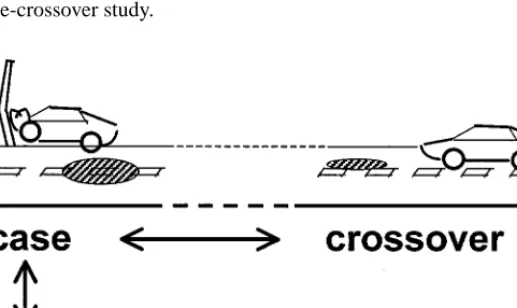
The simplest case-crossover design is closely analogous to a traditional matched-pair case-control design (Figure 1). In both designs, each case has a matched control. In a traditional matched-pair case-control study, the control is a different person at a similar time. In the matched-pair case-crossover design, the control is the same person at a different time, such as the same time on the day before the collision in the car phone study. This seemingly small paradigm shift, from control persons to control times, often has challenging consequences. Although many of the methodologic issues are the same as for traditional case-control studies, our experience with conducting case-control studies did not fully prepare us for doing a case-crossover study.
Figure 1 The relation of the simplest crossover design to a traditional matched-pair case-control design. Here the case, a collision at noon today, was exposed to a hazard, such as a puddle or cell phone call (shaded ellipse). How unusual was this exposure? To answer this question for all cases, a control group is needed. Instead of using a different car at the same time (bottom left), the same car at noon yesterday (top right) can be used as a matched control. Multiple previous control times also can be used to better estimate how often the car normally crossed back and forth between hazards and what fraction of previous driving times was exposed. If traditional controls (bottom left) are included in the study, their exposures at previous times (bottom right) can also be measured to estimate the magnitude of information bias or potential confounding by factors that vary over time.
?
What Problems Can Be Investigated by
a Case-Crossover Study?
Acute Cases The more abrupt the onset of the outcome, the more amenable it is to a case-crossover study because a time of onset is needed. Thus a vehicle collision or an injury that happens within 1 s can often be timed so accurately that triggers occurring just minutes before can be studied. However, triggering of diseases with insidious onset can still be studied by expanding the scrutinized case window, the window of observation when triggers are expected to be seen. To study risk factors for hemorrhagic fever with renal syndrome among soldiers in Korea, Dixon (5) made the case window extend from 7 to 34 days before hospitalization and the control window from 35 to 60 days before hospitalization.
In our MI study (29), we initially included all patients, whether the onset of symptoms was sudden, stuttering, or insidious. In the continuation of the study for another four years, we excluded patients with stuttering onsets and insidious onsets because questions about timing of potential triggers for vague or multiple onset times were difficult to ask, answer, and record. MIs with indistinct onsets were excluded from our analyses of triggering by exertion, anger, and sexual activity, but we could include some of them in analyses of life events, such as the death of friend, relative, or significant person (27), in which we use one-day exposure windows.
Crossover A basic requirement is that at least some subjects must have crossed at least once from lower to higher exposure or vice versa. The minimum amount of crossover is exemplified by the death of a spouse. This is a one-time, irreversible, unidirectional change in exposure status. [We found nine deaths of friends, rela-tives, or significant persons in the 24 h before MI onset, compared with five such deaths in the period 25–48 h before onset and three per day in the period 8–28 days before onset (28)]. Thus the measured exposure variable need not be transient, only its effect.
Crossover can be gradual, as illustrated by Suissa’s study (50) of fatal or near-fatal asthma. He looked at use of beta-agonists (drugs for constricted airways) during the 365 days before hospitalization or death (the case window, which he called the current period), compared with 366–730 days before hospitalization or death (the control window, which he called the reference period). In one analysis, crossover was defined as a change from low use (≤12 canisters/year) to high use (>12 canisters/year) of beta-agonists or vice versa. Out of 129 cases of fatal or near-fatal asthma, 29 were classified as high users in the case window but not the control window (“discordant exposed”) and, conversely, 9 were high users in the control window but not the case window (“discordant unexposed”). The ratio of exposed to unexposed discordants was therefore 3.2 (29/9), which is an estimate of the relative risk (RR) as in a standard simple analysis of a matched-pair case-control study. The remaining 91 patients, who were high users in both periods (“concordant exposed”) or low users in both periods (“concordant unexposed”), Annu. Rev. Public. Health. 2000.21:193-221. Downloaded from arjournals.annualreviews.org by University of Minnesota - Twin Cities - Wilson Library on 08/18/10. For personal use only.
?
dropped out of the analysis just like the concordant pairs in a matched-pair case-control study. In general, if people do not cross between exposed and unexposed, they do not contribute to the RR estimate.
Transience of Effect If the exposure itself is not transient, one or more of its ef-fects should be, otherwise no difference is expected between the exposure frequen-cies in the case and control windows. Transience is assessed from the perspective of the exposed people. For example, a driver’s exposure to a confusing intersection may last only 30 s, although the intersection exists continuously. Conversely, an exposure may be brief although its effect is prolonged, such as a 1-min telephone conversation that bothers the driver for the next 15 min.
The meaning of transience varies not only among different exposures, but also among effects of a single exposure. One exposure can influence risk by several causal pathways, each with separate transient effects and different effect-time re-lationships. An immediate severe effect that rapidly passes may be followed by a milder, long-lasting effect that eventually fades to nil. These separate effects can be in opposite directions. For example, the elevated risk of MI immediately after an episode of strenuous physical exertion, for which we found an RR of 2.4 (1.5 to 3.7) among people who regularly exercise strenuously, is presumably superimposed on the small contribution by each episode to a cumulative training effect, which reduces the risk of MI in the long term. A graph of risk over time, after patients start a regular exercise program, would show periodic spikes on a gradually declining slope (similar to Figure 1 in 45). The opposite situation—a hypothesized harmful long-term effect of beta-agonists coexisting with a known beneficial short-term effect—was investigated by Suissa (50). Separating acute effects from more chronic effects of a given exposure is one of the main rea-sons for using a case-crossover design. Suppose a daily drink of alcohol affects MI risk by a chronic effect on lipoproteins and an acute transient effect on fib-rinolysis. To estimate the magnitude of its acute effect, it would be necessary to remove self-confounding, the confounding of the alcohol’s acute effect by its chronic effect. Using cases as their own matching controls equalizes past alco-hol intake. For example, the traditional case-control study by Jackson et al (15) yielded an odds ratio among men of 0.75 (0.62 to 0.90) for alcohol intake during the 24 h before onset of nonfatal MI, compared with a comparable 24-h period in matched controls. This is consistent with the well-established inverse associa-tion between alcohol intake and MI, which could be caused by a combinaassocia-tion of ethanol effects—a chronic cumulative protective effect plus a repeated transient protective effect. Jackson et al subsequently did case-crossover analyses (24) comparing intake during the 24 h before MI onset with the usual frequency of alcohol intake among cases, by using various assumptions about cases’ patterns of past alcohol intake. They produced RR estimates ranging from 0.48 (0.27 to 0.84), if they assumed that drinking was extremely regular (e.g. that daily drinkers never missed a day), to 1.88 (1.35 to 2.61), if they assumed that drinking days were randomly distributed. In our study, we found that drinkers often reported Annu. Rev. Public. Health. 2000.21:193-221. Downloaded from arjournals.annualreviews.org by University of Minnesota - Twin Cities - Wilson Library on 08/18/10. For personal use only.
?
regular patterns of weekend vs weekday drinking, which favors an intermediate estimate. Using alternative methods of case-crossover analysis, we found no as-sociation between alcohol and MI in our data (22) after removing patients with vague premonitory symptoms who may have avoided alcohol after their symptoms began.
What Is a Trigger?
In a research proposal, the background section needs to be clear about the meaning of a trigger and the public health or clinical value of discovering more about triggers. It has been suggested that a trigger should be distinguished from an etiologic agent because it may merely advance the timing of an outcome that would happen soon anyway (39). This is misleading. The difference between earlier and excess cases is scientifically and legally important (11), but it is not what distinguishes triggers from chronic risk factors.
We have come to the conclusion that trigger is an entirely relative term. It means a more proximal cause. It can be used to describe any component (42) of the causal web that is closer to the onset of the outcome than most of the other component causes under consideration. Thus, depending on the overall exposure window of interest, each of the following causes can be regarded as a trigger of a vehicle collision: the distracting thought a half second before impact, the confusing intersection that the driver entered 10 s earlier, the short angry telephone call 5 min before the intersection, the decision to turn on the telephone 10 min earlier, the drink of alcohol 1 h before driving, the lack of sleep the night before, the start of a course of benzodiazepine taken for the first time on the preceding day, the death of the driver’s husband 3 days earlier, her exhaustion during the last week, and his move to a hospice 1 month before, which entailed her daily trips on roadways more hazardous than her usual routes. All of these factors could be identified as triggers in a case-crossover study.
What Is the Significance of Studying More Proximal Causes?
Knowledge of causes is useful if it enables better prediction of outcomes, elimina-tion of susceptibility (necessary cofactors), or reducelimina-tion of risk by modificaelimina-tion of the cause itself. Are triggers different from other causes in any of these respects? The answer appears to be no. One cannot generalize about the public health or clinical relevance of studying triggers rather than more distal causes. It is true that a trigger is sometimes a very predictive [nearly sufficient (42)] cause because it is most proximal to outcome onset. For example, a collision at high speed is very predictive of an injury. However, in general, a proximal cause might not be any more predictive, more necessary, or more manipulatable than any other component cause. A sudden fog on a busy highway is a highly predictive, but unmanipulat-able and unnecessary cause of a collision. A traffic signal with a faulty yellow light is a very manipulatable, but unpredictive and unnecessary cause. Driving Annu. Rev. Public. Health. 2000.21:193-221. Downloaded from arjournals.annualreviews.org by University of Minnesota - Twin Cities - Wilson Library on 08/18/10. For personal use only.
?
within five car lengths of the car in front is a nearly necessary cause of rear-end collisions in city traffic, but it is relatively unpredictive and unmanipulatable (i.e. unsustainable, because other vehicles quickly enter a five-car-length gap).
The significance of triggers depends on their frequency and duration of effect. If they seldom happen and are short in duration, then their impact on the cumulative long-term RR may be very low. With regard to frequency, we estimated that the doubling of MI risk in the 2 h after sexual activity would translate into a negligible annual RR of only∼1.01 among people who have sexual activity once per week (32). Concerning duration of effect, although the RR of a collision after a telephone call may be similar to that for a drink of alcohol (38), the effect of the drink may last 1 h compared with a few minutes for the phone call. Therefore, alcohol is the more important exposure to prevent. By similar reasoning, the transient hazard of physical exertion is worth risking for the more chronic training effect.
In contrast to MI, many of the chronic behavioral risk factors for vehicle colli-sions and occupational injuries, such as a risk-taking personality, are notoriously difficult to influence. Therefore, preventive actions may be more profitably aimed at reducing the hazardousness of transient environmental exposures, such as am-biguous intersections or occasionally used, ergonomically awkward tools.
Can Transient Preventive Effects Be Studied?
Preventive factors with transient effects are the opposite of triggers. We call them deterrents. For example, if the above-mentioned estimate of 0.48 (0.27 to 0.84) for the RR of MI from ingesting alcohol in the preceding 24 h were true (24; assuming perfect regularity of past alcohol intake), this would suggest that alcohol deters MIs for several hours. Similarly aspirin is hypothesized to deter MIs for several days by reducing the ability of platelets to aggregate. The deterrence wears off as the platelets that are exposed to aspirin are replaced by new platelets. This hypothesis can be studied in our MI data with exactly the same types of analyses as if it were hypothesized to be a trigger.
When a deterrent is taken regularly, one can treat an interruption in the deter-rence as a trigger. For example, the hypothesized surge in risk of MI associated with occasions of forgetting to take an antihypertensive, that is, longer “drug holidays,” might be detectable in our data. (In practice, it is hard for patients to remember instances when they forgot something, so ruling out negative-recall bias may be difficult.) In the rest of this review, the reader should assume that what holds for triggers also holds for deterrents unless we state otherwise.
How Should a Causal Hypothesis about a Trigger
Be Formulated?
We believe that the best way of expressing the causal hypothesis is to focus on the exposed cases. Then use a counterfactual conditional statement (23) adapted Annu. Rev. Public. Health. 2000.21:193-221. Downloaded from arjournals.annualreviews.org by University of Minnesota - Twin Cities - Wilson Library on 08/18/10. For personal use only.
?
for case-crossover studies: “Some exposed cases would not have occurred at that time, if they had not been exposed immediately before.”
This way of stating the causal hypothesis reflects the fact that case-crossover studies by themselves are unable to distinguish between an early case and an excess case (11). Likewise, they cannot distinguish between a deferred case and an avoided case. However, additional knowledge of the mechanisms of onset often permits us to do so. For example, because we know a great deal about how collisions happen, we know it is absurd to suggest that a car-phone call causes an inevitable collision to occur one day earlier than if there had been no phone call. By contrast, the hypothesis that sexual activity merely hastens the onset of an MI that inevitably would happen within a few days, triggered by merely walking up several flights of stairs, is reasonable. If the doubling of risk within 2 h of sexual activity is entirely caused by hastening MIs that would have happened next week, then the annual RR would be 1.00, not 1.01 as stated above.
It should be noted that all epidemiologic studies, even randomized controlled trials, cannot distinguish early from excess cases or deferred from avoided cases (11). However, the meaning of “early” depends on the length of follow-up. A 1-year trial can demonstrate a reduction (or excess) of cases during the 1 year of follow-up, but it cannot rule out the possibility that the reduction (or excess) was caused by deferral (or advancement) of cases to (or from) year 2. The distinction between earlier and excess is often semantic. Most epidemiologists probably would agree that an MI that occurs 5 years early should be regarded as an excess MI, but one that occurs only 5 days early should not be so regarded. Because case-crossover studies examine causation over shorter periods, they are more susceptible to this general weakness of epidemiologic studies.
How Should the Causal Hypothesis Be Quantified?
The above formulation of the causal hypothesis can be quantified as the ratio of the observed number to the expected number of exposed cases. The expected number may be very difficult or impossible to estimate. Consider the challenge of estimating it among constant drinkers who have injuries. They are concordant for alcohol exposure in the case and control times. If one tries to find a traditional control person, matched with each case based on past alcohol intake, the same problem arises; the matched pair is highly likely to be concordant for drinking on the day of the injury. Therefore, the causal hypothesis is tested in only a subset, the discordant patients. In the Missouri study of alcohol and injuries (52), there were 30 people who had one or more drinks on the case day but no drinks on the preceding control day vs only 12 who drank on the control day but not the case day. Assuming drinking yesterday has no influence on today’s risk of injury (which may be false, considering hangovers from heavy drinking yesterday), the number 12 is an estimate of how many patients would have been exposed on the case day if there were no acute causal relationship between alcohol and injuries. Annu. Rev. Public. Health. 2000.21:193-221. Downloaded from arjournals.annualreviews.org by University of Minnesota - Twin Cities - Wilson Library on 08/18/10. For personal use only.
?
The observed-to-expected ratio of 30/12 gives an estimate of 2.5 for the RR among this subset of drinkers. Unfortunately this may not be representative of the RR for the daily transient effect among constant drinkers.
FEASIBILITY STUDIES
What Determines Whether an Interview Study Is Feasible?
If a case-control interview study is feasible, a case-crossover study usually will be. We recommend doing a pilot study to test (a) the feasibility of recruiting patients rapidly enough for them to be able to recall the day of their event, (b) patients’ ability to recall their exposures on control days and/or their usual frequency of exposure, and (c) whether the interview data can be translated into case-crossover analyses with sufficient numbers of discordant patients. If a pilot study is not possible, we recommend contacting investigators who have done a case-crossover interview study that most resembles the proposed study.
Can Administrative Databases Be Used?
The Toronto (38) and Dundee (2) collision studies both involved linkage of ad-ministrative data: police records, a telephone company’s billing data, and a re-search database derived from drug dispensing data. Some case-crossover studies (1, 25, 49) have been done entirely within one database. A common problem with studies based on administrative data is lack of data on confounders. A big part of this problem disappears when cases are used as their own controls. With self-matching, one does not need data on relatively constant characteristics, such as a patient’s average health status and chronic risk factors. In studies of vaginal candidiasis (using start of vaginal preparation of an antimycotic agent) in relation to antibiotics (1) or the dermatologic drug acetritin (49), women’s usual patterns of sexual activity and genetic predisposition to vaginitis were controlled by self-matching.
Sequence symmetry analysis, first proposed by Petri et al (35) and used by Sturkenboom et al (49) and Hallas (13) as a method to explore prescription drug data, can be interpreted as a special type of case-crossover analysis. It can also be used to explore other heath services databases. If one of a pair of drugs (or health services) sometimes causes the other, the sequences of the two drugs in individuals who had both will be asymmetric. That is, people who started the hypothesized causal drug [e.g. an antihypertensive (13)] before the hypothesized outcome drug [e.g. an antidepressant (13)] will outnumber people with the opposite sequence of starting. This is like a reverse-direction matched-pair case-crossover design because the control window comes after the case window. Here the case window is a long period of various lengths before the outcome drug is started, and the control window is a similar period after the outcome drug. Causal inference is Annu. Rev. Public. Health. 2000.21:193-221. Downloaded from arjournals.annualreviews.org by University of Minnesota - Twin Cities - Wilson Library on 08/18/10. For personal use only.
?
limited by the potential for reverse-causation bias and confounding by fluctuating (within-person and between-time) indications or contraindications, which must be considered in all case-crossover analyses of databases.
DESIGN: THE STUDY BASE
What Are the Target Person Times?
When a promising population has been found, the theoretical target population should be defined (23). In a case-crossover study, this entails answering not just “What is the population at risk?” but “What are the person times at risk, that is, times in which an outcome could physically happen and be included in the study (under ideal circumstances of case finding)?” In the collision studies, the target person times at risk were driving times. It was physically impossible for the drivers to be involved in collisions during times spent outside their cars and almost impossible while they were parked. Times spent not driving were theoretically not part of the target person times. In the study of car phone calls and collisions (38), the investigators interviewed the discordant subjects to ascertain whether they had been in their cars at the same time on the day before their collision, a control day. In contrast, the Dundee study (2) of 1731 first collisions among drivers who had used psychotropic medications at least once during a 3-year period was unable to ascertain whether the people had driven on control days. Control days were the same days of the week as the collision days, during the preceding 18 weeks, regardless of whether the person had used a car. Thus, there was a discrepancy between their theoretical target and their actual person times. If people drove on only 90% of control days, this might explain the RRs of 0.93, 0.85, and 0.88 for tricyclic antidepressants, selective serotonin reuptake inhibitors, and other psy-chotropic drugs, respectively, compared with the RR of 1.6 for benzodiazepines. Retired people do not commute to work so they are less likely to have driven regularly on control days. Therefore, the discrepancy between target and actual person times would be greater for the elderly. This might partially explain the RR of 0.93 for benzodiazepine exposure among the elderly, compared with the RRs of >2 among people<45 years old. If Barbone et al (2) had obtained data on driving patterns in the control times by telephoning a sample of elderly drivers, they might have been able to adjust this estimate.
What Is the Study Base?
The concept of the target population is then operationalized as the study base. This may be the most challenging part of one’s research proposal because, rightly or wrongly, reviewers may think that some case time or control time selection biases have been overlooked.
The target person times of the child pedestrian injury study (40) were times when children cross streets in Auckland, New Zealand. The authors wisely chose Annu. Rev. Public. Health. 2000.21:193-221. Downloaded from arjournals.annualreviews.org by University of Minnesota - Twin Cities - Wilson Library on 08/18/10. For personal use only.
?
to restrict their study base to street crossings during children’s journeys to and from school. Note that some children contributed more street-crossing times than others, because their routes crossed more streets. We can imagine several different ways of precisely defining this study base: person times spent crossing the street, person distances on crosswalks, or individual crossings as if each crossing were the same duration and distance. Each definition relates to a slightly different version of the causal hypothesis. The authors chose the third definition, making the simplifying assumption that busy streets have the same width as quiet streets. If busy streets were twice as wide and required twice as much time to cross as quiet streets, then their reported RR of 6.3 (2.1 to 18.8) may have overestimated the effect of traffic density by a factor of about 2. We also wonder whether child times spent walking along rather than crossing streets were inadvertently included in their case times but not their control times.
In a study of antibiotic use as a trigger of vaginal candidiasis (1), with initiation of an antimycotic agent as a proxy for disease onset, we found that the distribu-tion of inducdistribu-tion times had modes at multiples of 7 days. This was because the timing of both antibiotic and antimycotic prescriptions was influenced by lack of access to general practitioners and pharmacists on weekends in Denmark. One approach to eliminating this bias might be to introduce different time restrictions on the study base, depending on the day of the week of the antimycotic agent (19). The study base can be confusing when there is a long induction time between the trigger and the outcome (48). In his study of hemorrhagic fever with renal syndrome, Dixon (5) included cases only if they were hospitalized in Seoul during the months of October through January. Patients were interviewed about their exposures during the preceding 60 days. The last 7 days were excluded to allow for a long induction time and referral process. The other 53 days were split about equally into case and control periods. Thus, for a patient hospitalized on October 1, the exposure window from August 28 to September 24 was taken as the case period and the window from August 2 to 27 was taken as the control period. Al-though the theoretical target person times would be defined as beginning with an infection in September and ending when the last infection began in mid-January, the base person times were between October 1 and January 31. Because of the in-duction time, some of the exposure window was necessarily outside the study base. This is consistent with the established practice in occupational cancer studies (48) for handling the first 2 decades of exposure, which cause increased cancer rates 20 years later. The first 20 years are excluded from the study base, but included in the exposure history. In the hemorrhagic fever study, the question of whether early August—the control period for patients hospitalized in early October— was too far outside the study base is not easy to answer. We discuss it further below.
The study base can also be confusing if it is interrupted rather than continuous, like driving times in the study of car phone calls and collisions. For example, a study of catastrophic injuries among racehorses (6) should have used horse distances rather than horse times as the study base. The authors had a difficult Annu. Rev. Public. Health. 2000.21:193-221. Downloaded from arjournals.annualreviews.org by University of Minnesota - Twin Cities - Wilson Library on 08/18/10. For personal use only.
?
hypothesis to test: There exists a carry-over effect between races, such that horses with insufficient recovery times between races are at increased risk of injury during the next race. This hypothesis can be expressed as the question of whether the risk of injury per horse furlong increases if the furlongs per month are increased (or, similarly, if the durations between runs are shortened.) By assuming that the study base was horse months, the authors substantially overestimated the RRs. They did not account for the fact that, even if there is no carry-over effect, horses that run twice as far during 1 month are twice as likely to be injured, because they have twice as large a base of horse distance in which injuries can occur.
The MI study by Hallqvist et al (14) was a case-crossover study nested within a population-based case-control study. Hallqvist (personal communication) pro-posed that the base of the case-crossover study was other people at the same time: the general population of Stockholm during the 1 h before each heart attack in that population. This is the standard study base for a traditional case-control study, except that it is restricted in time. We see this as the first of three possible study bases: (a) the population base, comprising all simultaneous person times at risk in the geographic catchment area (a “vertical slice” through population time); (b) the case history base, comprising all preceding (and sometimes future) times when persons can become cases during the catchment time window (a “horizontal slice” through population time); or (c) the population history base, comprising all simul-taneous and preceding (and sometimes future) person times in the population at risk in the catchment area and catchment time (an entire rectangle of population time, as illustrated in Figures 2 and 3 in reference 45). Which of these study bases is better for a given hypothesis depends on how well each one permits the counterfactual expected number to be estimated.
When Is a Case History Base Better Than a Population Base?
We did an n-of-1 case-crossover study (20) of hypothesized triggers of repeated syncope experienced by Kenneth Maclure (MM’s father), who was diagnosed with sick sinus syndrome and died of fatal MI at age 73 during a morning swim, after several other potential triggers. The target person times were Kenneth’s 62nd–74th years (and subsequent years if he had lived longer). The study base comprised the years 1980–1981 and 1986, during which there were 33 instances of syncope. We restricted the study base to those years because his wife, Margaret, was willing to review only 3 years of her diaries because the memories rekindled her grief. We had no intention to generalize the findings to other individuals, only to other years. Our goal was to identify triggers to which Kenneth may have been susceptible and to test Margaret’s general hypothesis, “Perhaps I should have done more to help him avoid stress.” Hypothesized triggers included visitors to the home, trips out of town, eating out, unusual exertion, and so on. The 24-h period before an episode of syncope was classified as a case day. Each case day was matched with a control day, the same 24-h period 2 weeks before. Margaret was surprised by our null findings and relieved of some lingering feelings of guilt.
?
To make up for the shortage of exposed case days, we might have looked for other patients with a similar recurring syncope and available diaries and pooled their experience with Kenneth’s. This would involve an assumption that the ad-ditional people had similar susceptibilities to triggers. If Kenneth’s susceptibility differed from that of most syncope patients, then a population base—other people at similar times—would have been problematic.
When Is It Appropriate to Use Both Study Bases?
The previously mentioned study of hemorrhagic fever in Korea used both a pop-ulation and a case history base (5). The question could be formulated either as “Why did these people develop the fever, whereas other people at the same time (in the population base) did not?” or “Why did these people develop the fever now rather than a month or two ago (in the case history base)?” To answer the first question, Dixon used a traditional case-control design. To deal with the problem that his hospital control group (which included a mixture of other illnesses and originated mostly from Seoul) might be unrepresentative of the population base, he also did a case-crossover analysis that answered the second question. By using both methods, he was able to refute more alternative explanations (selection bias and recall bias) than by using either design alone.
The case-crossover analysis included control times when people could not have become captured cases in the study. Cases were enrolled only during the epidemic months, October to January. The control times for cases hospitalized in early Octo-ber were the early weeks of August. However, an infection in early August that led to hospitalization in September would not have been captured as a case in the study because September was not within the study base. For this reason, should early cases have been excluded? Not necessarily. In every case-crossover study in which the control window precedes the case window, the first patient’s control window is outside the case catchment time. However, this is a problem only if there are major time trends in exposure frequency and if the exposure window is large compared with the case catchment window. Both of these conditions existed in Dixon’s study. If Dixon had kept October cases for his case-control study but excluded them from his case-crossover analysis, then the control times all would have been within his case catchment window. By including October cases, his case-crossover analysis may have underestimated the RR for living in tents, if living in tents was more common in August but safer because rodents did not enter seeking warmth.
How Do You Choose Between Alternative Study Bases?
The ideal study base is one with no confounding by other causes nor an imbalance of susceptibilities or necessary cofactors. For example, a randomized control trial of restrictions on phone calls in a large fleet of delivery vehicles would be ideal because other causes and cofactors would tend to be balanced. In the absence of randomization, the better study base is the one that is more similar to the case time in terms of major background causes, susceptibilities, and cofactors.
?
In the case of car collisions, the confounding by unmeasurable driver char-acteristics, such as risk-taking personality, is believed to be serious in compar-isons between drivers. So the past driving time of people who have collisions is usually the better study base. The opposite would hold if person/between-time variations in susceptibility and confounding were much greater than same-time/between-person variations and confounding. For example, to study car phone calls and collisions that occurred during a freezing rain storm, the case history base would be unrepresentative owing to the weather difference, and the population base would be less confounded because the within-day/between-person variation in risk-taking behaviors may be reduced if everyone is driving more cautiously.
Sometimes both past and simultaneous person times can be used interchange-ably. A study of mental stress and myocardial ischemia (12) used a population history base for data collection and initial analyses, but a case history base for the final analyses. (It is noteworthy that the case history of a patient with 20 ischemic events in 48 h resembles our n-of-1 study.) When these authors pooled data across all people and all times (as in their figure showing that ischemia was crudely asso-ciated with tension, frustration, and sadness in the 2760 h of monitored follow-up), they assumed that control times from different people were interchangeable with control times from cases (i.e. they used a population history base). This assump-tion appeared to be reasonable. From the figure and text, we estimate that the crude exposure odds ratio for tension over the entire population history of 2760 h was 2, very close to the exposure odds ratio of 2.2 (1.1 to 4.5) from the case-crossover analysis, adjusting for time and physical activity.
DESIGN: SAMPLING THE STUDY BASE
Why Sample the Study Base Rather Than Including It All?
There is no sharp line between a case-crossover study and a crossover cohort study. If one includes all of the past person times of cases—the entire case history base, then the study can be regarded as a crossover cohort study. If one has good data throughout the case history base, it is possible to invert one’s perspective and look at the data from cause to effect. For example, Farrington’s case-only study (7) of adverse events after measles, mumps, and rubella vaccination was restricted to patients who had both vaccination and an adverse event of interest—aseptic meningitis or convulsions with normal cerebrospinal fluid assay. The only question was the timing of the adverse events compared with time of vaccination, which Farrington treated as time zero. Likewise, in the study of antibiotics and vaginal candidiasis described above (1), all patients had used an antibiotic once and an antimycotic agent once. Time zero could be the start of antibiotic treatment, and the subsequent epidemic curve of antimycotic use could be examined as a crossover cohort study. Alternatively, time zero could be the start of antimycotic treatment, and prior timing of antibiotics could be examined as a case-crossover study. Annu. Rev. Public. Health. 2000.21:193-221. Downloaded from arjournals.annualreviews.org by University of Minnesota - Twin Cities - Wilson Library on 08/18/10. For personal use only.
?
A more complete crossover cohort study includes people who cross between exposed and unexposed times, but never become cases. They permit you to calcu-late a risk difference (RD) rather than just an RR. [An RD can also be estimated if a traditional control group is included and the sampling fractions of cases and controls are known, as in the Swedish study (14) of triggering of MI.] The simplest crossover cohort study is a before-after or an interrupted time series (4) in which the whole cohort simultaneously crosses once. The study of mental stress and myocardial ischemia (12) helps clarify the relation between a crossover cohort study and a case-crossover study and their relative strengths and weaknesses. A crossover cohort study has exposure information for the entire collection of person times at risk, not just for a sample of those person times (the control times). This prevents control-time selection bias. In the ischemia study, the analysis focused on 58 patients monitored for∼48 h, giving a total of 2760 person hours at risk, in which 388 episodes of ischemia occurred. Data on physical exertion and mental state were available for almost every waking hour. For sleeping hours, patients were assumed to be unexposed. Thus the investigators could divide the whole population history base into exposed and unexposed person hours and calculate an hourly risk in each: “Almost 40% of hours associated with heavy activity in-cluded ischemic episodes compared with less than 10% of hours associated with no activity” (12:1524). This translates into an RR of 4 and an RD of 30%.
If the data collection is prospective, one can avoid recall bias. This was a virtue of the ischemia study. The principal disadvantage is inefficiency. The ischemia study collected data from many subjects who contributed little or nothing to the analysis: those who had no outcomes (72 of 132 monitored for 48 h had no ischemic episode) and those who were concordant for the exposure of interest (30 of the 58 included in the analysis had no heavy exertion). The above-mentioned RD of 30% for heavy exertion probably would have been half as large if the 72 subjects with no ischemic episode were included in the denominator. The unadjusted case-crossover odds ratio of 15.7 for heavy exertion was more than double the cohort’s crude exposure odds ratio of 6.0 [(40%/60%)/(10%/90%)], presumably because the 30 concordant unexposed patients were sicker, that is, more susceptible to ischemia during inactivity and more likely to avoid heavy exertion.
Instead of all patients recording their mental states about 100 times each during the 48-h follow-up period (about once every 20 min), the patients could have reported mental states just 30 times each, yet there would still have been>2 control times per case time for most patients. The authors might still have obtained good estimates of the exposure odds in the study base and therefore good estimates of the RRs. Of course, this gain in data collection efficiency from sampling the study base comes at the price of less statistical power. We explored the tradeoffs between five alternative methods of sampling the case history base of our MI study (27). We found that “usual-frequency” data on heavy physical exertion during the entire year before MI permitted estimation of an RR with a 95% confidence interval (4.5 to 7.6), less than half as wide as the interval (2.7 to 11.1) from the matched-pair analysis, using only the day before as the control time.
?
How Long Should the Sampled Person Times Be?
At some stage between the beginning of design and the end of analysis, the study base must be divided into person times. These are the units of analysis. For example, Roberts et al (40) chose street crossing as the unit of analysis. If one can anticipate the most desirable unit of analysis early in the study, that unit can be used for sampling the study base. However, if the extra data cost nothing, the study base should be sampled in a manner that allows for various possible units of analysis. The Toronto collision study (38) looked at several days of telephone records, but the final unit of analysis was a fraction of an hour. The length of person times sampled should be related to the length of the case window, which should be related to one’s hypothesis about the length of the hazard period.
What Is an Effect Period, a Hazard Period,
and an Exposure Window?
While reviewing these published studies, we saw more clearly the need to distin-guish between several types of person times. To help reviewers, we suggest that the following terms be used.
The induction time is the time between cause and effect in an individual, the time between a momentary trigger and the onset of the triggered outcome (e.g. latency period). Most case-crossover studies so far have studied effects that could have minimum induction times of nearly zero. An exception was Dixon’s study (5) of hemorrhagic fever, which allowed for an incubation period.
The effect period is the time between the minimum and maximum induction times in the population. When the minimum induction time is zero, the effect period equals the maximum induction time. The maximum induction time is analogous to the washout period in crossover experiments, after which carryover effects are hypothesized not to occur.
A hazard period is a time interval after a trigger begins, such as a road hazard, when a population experiences an increased risk of the outcome caused by the trigger. The hazard period equals the effect period plus the duration of the episode of exposure. If the exposure is instantaneous, the hazard period equals the effect period. When the triggers are not instantaneous, such as extended telephone con-versations or long episodes of exertion, the hazard period is longer than the effect period. The total hazard period may be divided into several hazard periods of different degrees of excess risk (Figure 1 in reference 18).
An exposure window is an arbitrary unit of observation. It is a window one chooses to look into, when one is stating the hypothesis, designing the questions, or exploring the data. If it is the window in which one hypothesizes that an excess of triggers will be seen, it is the case window. The thing one observes while peering in that case window is case time. We designed the MI interview so that we could use exposure windows as short as several minutes and as long as a few days, because we were uncertain how long the hazard periods were. Evidence Annu. Rev. Public. Health. 2000.21:193-221. Downloaded from arjournals.annualreviews.org by University of Minnesota - Twin Cities - Wilson Library on 08/18/10. For personal use only.
?
concerning mechanisms of MI onset, anecdotal reports of triggered MIs, and the circadian pattern of MI incidence suggested that hazard periods could range from seconds to days.
The estimated effect period or hazard period is usually imprecise because it incorporates not only variation among the induction times but uncertainty of the timing of the trigger and the outcome. For example, the collision study (38) estimated the effect period to be∼5–15 min after car phone use, meaning from a minimum of zero to a maximum of 5 or 15 min after the call. Although the time of the phone call was exactly known from the telephone company’s records, the timing of the collision could be estimated only imprecisely, using drivers’ recollections and police reports. For triggering MI, we found that the estimated effect period was ≤1 h for exertion (29), whereas for sexual activity (32) and episodes of anger (28), it was≤2 h. Hallqvist et al (14) made improvements on our interview, so that they could measure more precisely the timing of exertion compared with time of MI onset. They estimated that the excess risk remained for ∼45 min after exertion stopped. They also estimated that the maximum induction time for MI onset after anger was probably≤1 h (31).
Should Times When Exposure Is Impossible Be Excluded
from the Study Base?
A common temptation is to control for exposure opportunity (37), that is, to select control times so that they are similar to case times concerning the patient’s opportunity to be exposed. For example, the Toronto collision study (38) included, as one of several control days, the “maximal-use day,” which was “The day with the most cell phone activity of the three days preceding the collision...” (Figure 1 in reference 38). By selecting a control time when drivers had more opportunity to use their phones (because there was evidence that they had remembered to take their phones that day), the usual frequency of cell phone use was overestimated, so the RR was underestimated to be 3 instead of 4.
The various studies of triggers of cardiovascular events have all faced the ques-tion whether sleep time should be excluded from the study base. Willich et al (53) excluded sleep time; the others (12, 14, 29) included it. On first thought, it seems like a form of control-selection bias to include sleep time in the control person time, because people do not have the opportunity to be exposed when asleep. However, this is the fallacy of controlling for exposure opportunity (37) in a new disguise. Sometimes the opposite may be true; to exclude sleep time may introduce a se-lection bias if cardiovascular events at all hours of the night have been included among the cases. However, as long as the same restriction applies to both case times and control times, selection bias is usually avoided.
To understand the exposure opportunity fallacy in the case-crossover context, consider again the ischemia study (12) in which all events detected by Holter monitor in 58 patients observed for 48-h periods were included, even ischemic events during sleep. Exposure data were collected only during waking hours, Annu. Rev. Public. Health. 2000.21:193-221. Downloaded from arjournals.annualreviews.org by University of Minnesota - Twin Cities - Wilson Library on 08/18/10. For personal use only.
?
between 6 AMand midnight. Patients recorded their mental states at randomly chosen control times, when alerted by a programmed beeper that sounded on average 3.2 times per hour during their waking hours. There was no need to “control for exposure opportunity” by excluding sleep time from the control time.
The investigators had two choices. (a) They could do as they did; that is, they could include all recorded ischemic events. Thus the study base comprised 2760 person hours—∼48 h from each of the 58 patients, including sleep time—and the investigators had to make the assumption that patients were unexposed when their beepers were turned off. (b) Alternatively, the investigators could have restricted the study base to the waking hours during which exposure data were collected. We used the first approach in our MI onset study because our questions about exposure during the past 26 h included nighttime as well as daytime. The second approach seemed more difficult because detailed data on usual wake times and sleep times were hard to collect. A child injury study (36) used the second approach. Sleep time was excluded because few children are seriously injured falling out of bed while asleep.
“Controlling for exposure opportunity” is appropriate only if it is not an expo-sure of primary interest but a necessary cofactor or an important confounder or modifier that one certainly would control for. Driving was a necessary cofactor in the collision studies. Seasonal exposure to active virus in aerosolized rodent urine may be considered a necessary cofactor in the study of hemorrhagic fever; outside the epidemic season, living in tents may not be a risk factor. In our ongoing study of occupational hand injuries (46), we do not count injuries outside working hours (although occasionally an injury after work may be partially attributable to an unreported strain at work.)
The confusion about exposure opportunity arises partly from the need to equal-ize opportunities for outcomes between exposed times and unexposed times. Con-fusion is more likely when the exposure and outcome are similar. In the study of antibiotics and vaginal candidiasis described above (1), the exposure was the start of an antibiotic and the proxy for the outcome was the start of an antimycotic agent. Controlling for day of the week was necessary in that study because the opportunity to start an antimycotic agent was much less on weekdays when gen-eral practitioners’ offices were closed. If it had been a prospective study in which women reported vaginal symptoms immediately by telephone (and if starting an antibiotic was the only cause of vaginitis associated with day of the week), then there would have been no need to control for day of the week. Then the fact that the opportunity to start an antibiotic was greater on weekdays would be irrelevant.
Should Case Times Always Be Excluded
from the Control Times?
In a cohort study, all cases in the numerator are also counted as persons or person times in the denominator. In a nested case-control study, controls are sampled from Annu. Rev. Public. Health. 2000.21:193-221. Downloaded from arjournals.annualreviews.org by University of Minnesota - Twin Cities - Wilson Library on 08/18/10. For personal use only.
?
the denominator without excluding patients who eventually become cases. The same principle holds for case-control studies even when the underlying cohort is not well specified. By the same token, the denominators of crossover cohort studies include case times. The same is true for the control times of case-crossover studies. They are meant to represent the denominator of the corresponding crossover cohort. Therefore they do not need to be free of previous case times.
In the ischemia study (12), case hours were those with an ischemic event and control hours were non-case hours. The odds of heavy physical exertion vs in-activity were 36 to 230 in case hours and 54 to 2081 in control hours, giving a crude exposure odds ratio of 6. In contrast, the crude risk ratio was 4 (36 case hours among 90 h of heavy exertion, divided by 230 case hours among 2311 h of inactivity.) The exposure odds ratio overestimated the risk ratio because the rare disease assumption did not hold. If these researchers had defined control hours as the full study base, including both case hours and noncase hours, the rare disease assumption would not be needed. Then their crude exposure odds ratio would equal 4.
This does not mean that the index case time (as distinct from previous case times) should be included among the control times. For example, the Danish pilot study of whether media events trigger physician visits might be viewed erroneously as a retrospective cohort study with one continuous week of follow-up, because all patients were asked about their exposures to health information in the media during the week before their visit. It was tempting to count the case day as part of the denominator, which means it would be counted as both a case day and a control day. This would cause the RR to be underestimated, however. Only if the case history were very long, such as 1 year, would it be appropriate to view this as a retrospective crossover cohort study. Previous days with visits to a physician would not need to be excluded from the denominator (the control time). The index case time (the visit that caused the patient to be included in the study) also could be included if the entire case history were included in the denominator.
When Can Future Person-Times Be Used as Controls?
The ischemia study (12) and the air pollution studies (17, 34) used both past and future control times. Such bidirectional sampling (33) makes sense in studies of ambient air pollution because people’s past illnesses do not influence future am-bient air pollution levels (although they may influence people’s tendency to stay indoors or to leave town). A symmetric bidirectional design (e.g. selecting control days as 7, 14, 21, and 28 days before and after the case day) eliminates most of the bias from pollution trends over time (3). Studies of air pollution and daily mortality traditionally have used time series designs with increasingly sophisticated Poisson regression models to control for secular, seasonal, and weekly trends. Critics argue that such studies have depended too much on modeling assumptions. In response to critics, some researchers (17, 34) have used symmetric bidirectional case-crossover designs to control for time trends by design. They reanalyzed data Annu. Rev. Public. Health. 2000.21:193-221. Downloaded from arjournals.annualreviews.org by University of Minnesota - Twin Cities - Wilson Library on 08/18/10. For personal use only.
?
previously analyzed by Poisson regression and obtained almost identical results. They concluded that case-crossover designs are better suited to the study of ef-fect modifiers than Poisson regression of time series data, although they have less statistical efficiency (3).
SAMPLE SIZE
How Many Cases and Control Person Times
Are Needed for a Case-Crossover Study?
Less than half as many subjects may be needed in a case-crossover study as in a traditional case-control study because the same results may be obtained without the need to interview traditional controls, and each case can provide multiple control times. The most important determinants of sample size are the rarity of the trigger and/or the frequency of discordance, which are often unknown until a pilot study is done. If possible, efficiency may be gained by excluding cases with regular constant exposure or nonexposure and recruiting only patients with a high frequency of crossover. This is a form of counter matching (47), which increases the proportion of discordant subjects.
Are Case-Crossover Studies Inefficient
Because of Overmatching?
The concept of self-confounding between acute and chronic effects of exposures should help dispel the concerns of some reviewers that self-matching is overmatch-ing. Self-matching can be overmatching only if there is little or no confounding by unmeasured constant characteristics, nor much residual confounding by poorly measured constant characteristics. This will rarely happen if an exposure has both an acute and a chronic effect, because past exposure is usually highly correlated with recent exposure.
What Power Is Gained by Going from 1 to 4 to 100 Control
Times per Case Time?
A common rule of thumb is that little is to be gained from going beyond four controls matched to each case in a case-control study. This rule of thumb does not apply when the exposure of interest is rare, which is often the case with triggers. Thus, we (26) found that the confidence intervals of our RR estimates were reduced by∼35% in going from 1 to 4 control periods and by 40% in going from 4 to>100 control periods. Unlike a traditional case-control study, in which the cost of additional interviews limits the ratio of controls to cases, there may be no additional cost in a case-crossover study. For example, in our MI study, it cost nothing extra to ask about usual frequency during the past year, rather than during the past week.
?
DATA COLLECTION
What Has Been Learned About Questionnaire Design?
We limit our advice to four major points. First, although some questions are easy to phrase, one should expect the design and testing of the interview to be a challenge, especially if the effect period is uncertain. Second, we found that redundancy permitted validation checks that helped rule out recall bias. For alcohol, we asked about (a) usual frequency and time since last intake, (b) intake during the past 36 h, which we recorded by using a timeline, (c) usual weekly pattern of alcohol intake (e.g. weekends only, every Thursday, etc), and (d), among regular drinkers, usual frequency of abstaining for 24 h and time since last 24-h abstention. Third, we found that open-ended questions at the beginning of the interview are useful to assess whether patients have prior hypotheses that might cause reporting bias. But case-crossover analyses are not possible with open-ended questions because information is also needed on past exposure to the trigger from patients who did not experience the trigger just before their event. Fourth, on the brighter side, when the meaning of a phrase is subjective, such as “enraged: loss of control, throwing objects, hurting yourself or others” (28), it is reassuring that each patient will use the same definition for both case time and control time.
What Questions Are Needed When a Cofactor of
Interest Is Intermittent?
In a study of alcohol and injuries (52), alcohol is an intermittent modifier of risk. Exposures to hazardous objects are also intermittent. To assess the modifying ef-fect of alcohol, we puzzled over whether it was necessary to ask such specific ques-tions as “How often do you drink alcohol just before you use kitchen/workbench tools?” We concluded that such questions were not necessary to assess qualitatively whether alcohol increased or decreased the RR. However, to quantify accurately the magnitude of modification, we would need to ask an awkward question on the patient’s usual frequency of concurrent exposure to both alcohol and physical haz-ards. In the Dundee collision study (2), an RR of 8 (based on 7 exposed cases) was reported for benzodiazepine use concurrent with a positive breath test for alcohol at the time of collision. This estimate assumes that the people exposed to alcohol on the collision day were also exposed on all of their control days or that the odds of benzodiazepine use on control days was not related to alcohol use.
METHODS OF ANALYSIS
Alternative approaches to the analysis of case-crossover studies are described at length elsewhere (7, 8, 10, 18, 24, 26, 51a). We recommend that a research pro-posal emphasize the most familiar methods: Mantel-Haenszel estimates (18) with confidence intervals for sparse data (41), computed by using formula 12-58 in the Annu. Rev. Public. Health. 2000.21:193-221. Downloaded from arjournals.annualreviews.org by University of Minnesota - Twin Cities - Wilson Library on 08/18/10. For personal use only.
?
first edition of Modern Epidemiology (43) [formula 15-24 in the second edition (44)], and by using conditional logistic regression (26).
Reviewers of the proposal may expect familiarity with an important paper by Greenland (10) that gives a unified approach to the analysis of case distribution (case-only) studies. These include case-crossover studies, as well as two designs that use hypothetical rather than observed controls: genotype (16) and case-specular studies (54). Greenland’s method extends to case-crossover studies that include traditional (other-people) controls and use control-crossover analyses (see section on “Limitations” below). His point of departure is a case-crossover study with “usual frequency” data (26) that enable the exposure distribution in the entire case history base to be estimated (which is why Greenland likes the term “case-distribution study”). For example, in the MI study, we asked cases for their usual frequency of sexual activity in the past year. A future car phone study might ascertain the percentage of car travel time spent using a cell phone. In such analyses, there are no specific control times.
Greenland’s use of the terms “pseudo-controls” and “hypothetical controls” and the phrase “K-1 matched controls” can be misleading. At first glance, these terms seem to imply that control times in all case-crossover studies are false or hypothetical. Actually, Greenland is using the term “controls” in a novel way to describe the case history base. These controls are not control times of equal length. If applied to the Dundee study (2), which had 18 control days for each collision day, K-1 would not equal 18. K is the number of exposure levels. In the simplest analyses of the Dundee study, K was 2 (e.g. yes or no for exposure to benzodiazepine). For each case in such analyses, there would be only one pseudo-control—the aggregated past person times having the opposite exposure to the case time. This novel usage is likely to be confusing to some readers, so we translate the key formula into more concrete terms, as follows.
Greenland showed that the contribution to the joint likelihood from subject i could be written as
[exp(uc(i)diβ+wc(i)θ)ti c(i)] Á X
k
exp(ukdiβ+wkθ)ti k.
(We combine notation from Greenland’s Equations 5 and 16.) It is best to read this formula from back to front and bottom to top and to refer to Figure 2, in which we illustrate the terms. The sum of all person times when individual i is at risk is represented byPktik[e.g. travel times (the T shapes in Figure 2)]. The
term tikequals the amount or fraction of these times spent by individual i at the k level of exposure. (The log of tikis the individual’s offset in a conditional logistic regression analysis.) The simplest way to define k is to give it only two levels,
k=1 (e.g. a car phone call, shown in Figure 2 as a k-shaped cellular telephone) or k=0. In Figure 2, ti(k=1)is represented by the amount or fraction of roadway
that is shaded (e.g. the duration and aftermath of cell phone calls.) The ratio
ti(k=1)/ti(k=0)is the exposure odds in the case history base (the ratio of shaded to
unshaded road). The ratio ti c(i)/ti(k6=c)is the odds of either exposure or nonexposure. Annu. Rev. Public. Health. 2000.21:193-221. Downloaded from arjournals.annualreviews.org by University of Minnesota - Twin Cities - Wilson Library on 08/18/10. For personal use only.
?
Figure 2 A pictorial explanation of Greenland’s likelihood formula for case-crossover studies (10), using the example of car telephone calls and collisions as in Figure 1. Time moves from right to left. Objects are approximately shaped and positioned like letters in Greenland’s formula. Road segments (T shapes) are travel times that together make the study base when collisions are possible. The hypothesized cause, a k-shaped car phone, casts a shadow (the hypothesized hazard period) for the duration and aftermath of each call. The case window (top, large C shape) encircles case time immediately before damage to the D-shaped car driven by individual i, who has collided with a post shaped like the numeral one (illustrating Di =1 if a case). The length of
the case window can be arbitrarily increased or decreased to test hypotheses about the length of the hazard period. For a traditional case-control analysis, a control car (Di = 0) is sampled from the
population of different cars at the same time, and exposure is assessed in the catchment window (bottom, large C shape) encircling a control time immediately before sampling. In case-crossover analyses, control times are the same car at different times. Thus, one or more control times are sampled from the case’s history of travel times (catchment windows are not shown here), or else the entire case history may be included as control times, without sampling (as shown here). Level of exposure in the case time is shown by radio signals (w, u) meaning whether using the car phone. The dish on the tower (θ) represents a possible trend in cellular-telephone calls (average increase or decrease in the log odds of a call) as cars approach the tower and signal quality improves. If such a trend exists, it is likely to be a confounder. Because it affects the entire population history, it can be measured in a control-crossover analysis. The association of interest, shown as a sign warning drivers to beware of the bother (β) of calls, is the average increase or decrease in the log odds of a call during the case time (the antilog of which estimates the RR of collision associated with car phone calls.)