Detecting linguistic change based on word co-occurrence
patterns
Carmen Klaussner
Trinity College Dublin
Carl Vogel
Trinity College Dublin
Arnab Bhattacharya
Trinity College Dublin
ABSTRACT
Diachronic linguistic analysis focuses on detecting elements of language change over time. This change can take different forms, as for instance certain words could show a slow increase or decrease in frequency over time as these become more popular or obsolete. We are interested in sudden change in words that are attested for in every time slice of the overall examined time period. In particular, we are trying to relate the change in frequency of words that are alwaysthere to words that emerge around certain points in time and only remain frequent for shorter periods of time, suggesting they are more prone to sudden changes in popular topics or could be influenced by historical events. This addresses the question of how the more regular word expressions’ frequencies are influenced by new clusters of words appearing and disappearing. Although there might be links to collocation analysis, words that occur frequently next to each other are not of primary interest here, but rather words that are conceptually related, where one is causing or affecting the frequency of the other, which causes them vary in a similar fashion. We use statistical change point analysis for identification of significant change over time and seek to validate our findings by randomly extracting example sentences from the data.
KEYWORDS
diachronic analysis, language change, change point analysis
1
INTRODUCTION
Findings from temporal studies offer an important source of enrich-ment and validation for non-temporal studies, especially when one needs to disentangle (general) temporal effects from non-temporal ones, as for instance in the realm of stylometry and authorship attribution [2]. Change in linguistic variables can occur in differ-ent shapes and forms: slow gradual change as opposed to sudden and abrupt, short as well as long-term effects. Differences could be rooted in levels of linguistic abstraction, as for instance individual words are likely to show more variation over time than entire word classes, where smaller fluctuations would be averaged and only larger trends pervading the entire group would be more easily dis-cernible. Features are usually classified along one or more different dimensions, such as membership of either an open-or closed-class or according to the frequency strata, i.e. frequent, medium-frequent and rare, they belong to. However, even though these classifica-tions are often represented as categories suggesting there is a clear boundary between, for instance what is frequent and infrequent, a continuous representation, especially considering temporal effects would occasionally seem more suited. This is especially true in the realm of diachronic analyses, the analysis of texts over time, as most
items might appear across different frequency strata depending on the exact time period examined.
We aim to show that even the open-class/closed-class view of features might be insufficient when observed through the lens of temporal text representation. While something might bear the label of common noun, it could in fact be closer to a function word, behaving and being affected by similar factors, such as regular occurrence in different contexts.
In this work, we consider the analysis of the more regular and possibly also frequent items, in particular those appearing in all years of the time period examined. Typically, these features are more general in meaning (e.g. temporal expressions) rendering them suitable for a variety of language contexts other than strongly topic-related words, such ashurricaneorcomputer. Our main hypothesis is that these items change through other less frequent items that are more prone to topic change over time, such as concepts relating to the outbreak of a war or natural disaster. The type of change we are looking for is a change in mean, whereby a feature changes its relative frequency fairly abruptly at timet, rising or falling to a new level and remaining there for at least some time. If one compares the mean over the samples before timetto the mean taken over the samples after timet, one obtains significantly different means. This type of research has to be distinguished from two related areas of research, i.e. semantic change in the form of neologisms and collocation analysis. Semantic change analysis is different in that it considers cases whereby a word acquires a new sense and possibly also a second part-of-speech class and could subsequently be used in different syntactic contexts, whereas here we consider changes of word frequencies and their possible non-semantic change related causes, as for instance a particular temporal expression used for contrasting different situations, e.g.‘If I had only known then, what I know now.’Also, conceptually, these regular and irregular appearing words could be relatable through collocations or otherwise longer n-gram sequences. While the method presented here could be used for their detection as well, it is not limited to relationships between words that occur close to each other, but also words or expressions that only share a conceptual rather than spatial relationship, such as the first (‘Detecting’) and last (‘patterns’) word of the title of this work, that as 8-grams are rarely computed, is less likely to be captured by collocation analysis, while the terms are clearly conceptually related.
validation of these through the actual data. We discuss these results in section 7 and conclude the work in section 8.
2
PREVIOUS RESEARCH
Different areas of linguistic research consider the change of broader categories of words, such as frequency effects in syntax [1], largely distinguishing between type and token frequency of a particular variable or category. Bybee and Thompson [1] discuss three fre-quency effects that are important not only in shaping phonology and morphology, but also syntax; two effects are caused by high token frequency, which have adverse tendencies that can only be explained by considering the influence of the third frequency effect of high type frequency. A high token frequency of an item pro-motes its reduction, as visible in conventionalized contractions in English (I’m,can’t). In contrast, the ‘Conserving Effect’ is visible with high token items, where the more the form is used the more it is strengthened, compare normalization of the English past tense of ‘weep’ fromwepttoweeped, compared to high frequency items, such as ‘sleep’ (slept). A syntactic example of this is the fact that pronouns, although derived from full noun phrases show much more conservative behaviour (e.g. case marking) due to their higher frequency. The type of change that is resisted in the high token frequency items is change on the basis of combinatorial patterns or constructions that are productive. “The more lexical items that are heard in a certain position in a construction, the less likely it is that the construction will be associated with a particular lexical item” [1, p.384]. This is observable in the ditransitive construction, which is only acceptable with very specific lexical verbs of high frequency, compare: “ Hetoldthe woman the news” vs. “Hewhisperedthe woman the news” [1, p.385], where the verbtellis a lot more fre-quent thanwhispered. To a limited extent, this is also productive in that the construction can apply to a few new high frequency verbs, such ase-mailedortelephoned.
Hamilton et al. [4] consider the function aspect of diachronic change by taking a closer look at global and local shifts in a word’s distributional semantics in historical texts from English, French and German.1For the local orcultural shifts, they use a local neighbour-hood measure and for the global measure they compute the cosine distance between two word vectors capturing the co-occurrence statistics at consecutive time pointstandt+1. Based on previous results in the literature, they predict that nouns are more likely to undergo change because of cultural shifts, whereas verbs are more likely to change because of regular semantic change. Across all languages as predicted, the local neighbourhood measure assigns higher rates of semantic change to nouns than verbs with the op-posite applying to the global measure. This also remains the case, when adverbs and adjectives are included among the verbs, sup-porting previous results in the literature suggesting that adverbial and adjectival modifiers are often the target of regular or global linguistic change [4].
The research presented by Kulkarni et al. [7] considers change point analysis in the context of investigating statistically significant shifts of semantic change. They consider three different approaches,
1
Local or cultural shifts are deemed less regular and stable than global shifts, as they are caused by more changeable factors, such as new technologies, whereas global shifts are associated to regular semantic change, such as grammaticalization.
one frequency based, whereby sudden changes in word usage are captured. The second one involves asyntactictime-series analysis, analyzing word’s part-of-speech tag distributions and finally they construct a distributional time-series by considering contextual cues from word co-occurrence statistics. Using human evaluators to assess the performance of their models, they find the highest amount of agreement between annotators and method with respect to words that have undergone change is the distributional method with c.53% average agreement compared to c.22% (syntactic) and c.13% (frequency). Another change point oriented analysis was addressed by Riba and Ginebra [9], which investigates a possible change in authorship of Tirant lo Blanc, identifying a clear single sudden change point that is supported by cluster analysis. Our work examines possible changes in features that are both regular in occurrence and highly frequent caused by features that are only highly frequent over a short period of time, similar to semantic cultural shifts, but for the difference that these words would not necessarily take on a new meaning.
3
DATA
For this analysis, we consider a 100-year long extract fromThe Cor-pus of Historical American English (COHA)[3].2This is a 400-million word corpus, which contains samples of American English from 1810–2009 balanced in size, genre and sub-genre in each decade (1000–2500 files each). It therefore contains balanced language sam-ples fromfiction,popular magazines,newspapersandnon-fiction books, which are again balanced across sub-genre, such asdrama andpoetry.3
For this study, we selected all data from the years of 1880-1979 covering all genre ofnews,magazine,fictionandnon-fiction. For most of the experiments, we only use thenewssection of the data, as it is most likely to contain the types of change we are targeting, though occasionally comparing to the other three genre. In order to arrive at a relative frequency count for each feature, we combine the individual files on a per year basis and relativize by the overall token count for that year.4As features, we consider the set of word bigrams marked for syntactic context, e.g. the wordlikehas different meanings depending on its context. It can be used as both a verb and a preposition, which should subsequently be treated as two separate items. We chose bigram size as it provides more context and is richer in meaning allowing us to discern more specific items of change than with unigram size. We decided against analyzing items of higher rank and abstraction, such as part-of-speech sequences as these are more difficult to evaluate, while word sequences offer more possibilities for human evaluation.
In order to extract part-of-speech (POS) features needed for syn-tactic word features, we used the TreeTagger POS tagger [8, 10]. Our new syntactic word features were then created by using the tag sequence as a suffix to the original word in context that gave rise to it. Thus, “He likes her” becomes “he.PP likes.VBZ her.PP”.5Items
2
free version accessible on: http://corpus.byu.edu/coha –last verified July 2017.
3
There is an excel file with a detailed list of sources available on: http://corpus.byu.edu/coha/–last verified July 2017.
4
In the case of higher sequence features, such as word bigrams the unigram token count is replaced by the unique bigram token count.
5
In this, the difference between the original word in context and the lemma of the word would primarily be reflected in verbs.
are then joined to bigram sequences and each two syntactic word sequence is relativized by the total number of bigram sequences in that year. For this work, we are primarily interested in changes in common nouns, requiring us to extract these from all other types. We only retainadjective-nounornoun-nouncombinations, as we expect the other types that can occur in noun phrases, i.e. deter-miners, proper nouns and pronouns to follow a different frequency distribution that might introduce noise.
Figure 1: PCA results for the 10 highest associated bigrams.
last.JJ week.NN last.JJ year.NN next.JJ year.NN
good.JJ deal.NN young.JJ lady.NN few.JJ moments.NNS
young.JJ man.NN
first.JJ time.NN
many.JJ people.NNS
great.JJ deal.NN
−1.0 −0.5 0.0 0.5 1.0
−1.0 −0.5 0.0 0.5 1.0
pc1 axis
pc2 axis
4
METHODS
In this section, we describe the methods used for initial detection of interesting constant features, our data exploration and the change point analysis.
4.1
Detecting changing features
As we are interested in change in variables appearing in all time instances of a temporally-ordered data series, we consider only those bigram adjective-noun/noun-noun types that appear in all time slices and discard all others. Even when reducing the set of fea-tures to these constant noun types, some 350 sequences remain for examination. In order to discover interesting (and possibly related) features more easily, we first order them according to mean relative frequency and then use principal component analysis (PCA) on sets of 50 bigram features, as we have found estimation and later inter-pretation of components to be better, when the document-feature ratio is in favour of more samples. PCA is an unsupervised statisti-cal technique to convert a set of possibly related variables to a new uncorrelated representation or principal components. This type of analysis groups features according to common variance patterns and can help to detect features that vary in a similar way. The results of running PCA on the 50 most frequent noun-noun/adjective-noun
[image:3.612.323.567.254.572.2]sequences are 50 new components that group related features to-gether.6A feature can be negatively or positively related to a new component. The components themselves account for decreasing proportions of variance, e.g. in this case the first component ac-counts for 25% and the second component for 12% of the variance with the rest being more broadly spread out. Inspection of first principal component allows for discovery of the three highest as-sociated items:last week,last yearandnext yearwith very similar weights: 0.259558004, 0.256880159 and 0.252325884 respectively (Figure 1).
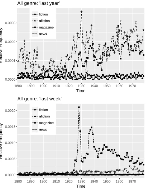
Figure 2: 19th/20th century corpus: word bigrams ’last year’ and ’last week’ shown over different genre types: news, mag-azines, fiction and non-fiction.
●●●● ●
●●●● ●●
●● ●●●●●●●●●●●
● ●●●●●●●●●●●●●
● ●●●●●
● ●
● ●●
●●● ●●
● ●●●●●●
● ●
●●●●●●●●●●●●●● ●
●●●●●●●● ●
●● ●
●● ●
●●●●●●●
0.0000 0.0001 0.0002 0.0003
1880 1890 1900 1910 1920 1930 1940 1950 1960 1970
Time
Relativ
e Frequency
● fiction
nfiction
magazine
news All genre: 'last year'
●●●●●●●●●●●●●●●●●●●●●●●●●●●●●●●●●●●●●●●●●●●●●●●●●●●●●●●●●●●●●●●●●●●●●●●●●●●●●●●●●●●●●●●●●●●●●●●●●●●●
0.0000 0.0005 0.0010 0.0015 0.0020
1880 1890 1900 1910 1920 1930 1940 1950 1960 1970
Time
Relativ
e Frequency
● fiction
nfiction
magazine
news All genre: 'last week'
Figure 2 shows two of the features:last yearandlast week. Both display rather sudden changes around 1920, albeit for different genre, ‘last year’ becomes more frequent in thenewsdomain and after thatmagazines, while for ‘last week’, the order is reversed: firstmagazinesand thennews.
4.2
Type-token analysis
In order to understand the underlying development in the data bet-ter, yielding a more informed analysis, we explore some methods
6
For this experiment only, we took logarithms of relative frequencies before applying PCA.
inspired from data analysis in the financial sector,Rate of Change (RoC). The methods described here are used in section 5. In par-ticular, we are interested in what way different groups of features change over time with respect to different quantities. For this, we consider two basic linguistic measures, type-token ratio (T TR) cal-culated as the number of types in a particular category divided by all the number of tokens and a type-vs-all-types ratio (TYPR), whereby we compare the number of types in a particular category to all types. Further we combine these two ideas with the RoC in order to gain insights in how types of features not only change over time, but are related to the respective previous time instance. The log RoC is defined as, the value of the variableVt today divided by the value yesterdayVt−1as shown in eq. 1. Thus, this
is showing how a particular value changes, for instance from one year to the next.
RoCln=ln
Vt
Vt−1 !
(1)
For most of the analysis, we use simple T TR and TYPR, except for figure 5, for which a slightly modified version of the RoC is used. Rather than having the current value at timet in the numerator, we consider the set of linguistic types that two time points have in common , as shown in Eq. 2. Thus,|typesy
t| ∩ |typesyt−1|refers
to the size of the group of features found in yearytandyt−1with
respect to the number of tokens inyt−1. The second version, shown
in eq. 3 relativizes with respect to the number of total types inyt−1.
In the following, we refer to these to measures as T TR’ and TYPR’ to distinguish these from static type-token ratios. As is common with financial data to achieve symmetry between decrease and increase, we take natural logarithms.
TT R′
yt =ln
|typesy
t|∩ |typesyt−1|
|tokensy
t−1|
!
(2)
TYPR′
yt =ln
|typesy
t|∩ |typesyt−1|
|typesyt−1|
!
(3)
These two measures allow us to observe how the broader cate-gories behave with respect to feature types and what proportion these take of either all types or tokens.
4.3
Change-point Detection
Change point analysis is the analysis of a time-series with the aim to detect specific pointstin time that separate the points before and after it with respect to some criterion. More formally, aspects of change point analysis can be defined as follows: given a time-series {yt : t ∈ 1, ...n}, a change point occurs if there exists a timek, where 1≤k≤n−1, such that the distributions of{y1...yk}and
{yk+1...yn}are different with respect to some criterion, i.e. change
inmean, change inregressionor change invariance. For this analysis, we are primarily interested in changes in mean as these would sig-nal a higher or lower average usage of a feature with respect to an earlier time period, while for instance a change in variance would indicate greater or lesser variability in how a feature is used. As we are interested in long-term change, that lasts at least 10 years or so we require a change point detection technique that is less volatile to short-term fluctuations in the data. For our experiments, we chose the approach by James et al. [5], originally used for breakout
detection in cloud data in the presence of anomalies.7The proposed approach (‘E-divisive with Medians’(EDM)) is a non-parametric technique using medians and estimating the statistical significance of a change point through a permutation test. We found this tech-nique to return fewer change points that were more spread out than distribution based change point methods, rendering it even more desirable as our data is not always normally-distributed. We found that using transformations occasionally smooths over interesting developments making these less desirable to use in this context.
5
DATA EXPLORATION
[image:4.612.320.555.345.481.2]In the following section, we look at unigram and bigram instances of both function and content types to gain an intuition about general trends in the data. We begin by exploring changes in type and token relations in unigrams of both a function (determiner) and a content (noun) category. For the determiner category, we considered both instances corresponding to⟨DT⟩and⟨WDT⟩, thus boththe.DTand which.WDTin contexts, such as‘Which/The book...’.
Figure 3: News corpus: determiner types divided by total to-kens(TTR) or types (TYPR).
●●●●●●●●●●●●●●●●●●●●●●●●●●●●●●●●●●●●●●● ●
●●●●●●●●●●●●●●●●●●●●●●●●●●●●●●●●●●●●●●●●●●●●●●●●●●●●●●●●●●●● 0.0000
0.0005 0.0010 0.0015 0.0020
1880 1890 1900 1910 1920 1930 1940 1950 1960 1970
Time
Propor
tion (%)
● TTR
[image:4.612.104.290.418.474.2]TYPR
Figure 3 shows the number of determiner types with respect to all types/all tokens over time. The top line shows a sharp decrease in 1920 for the determiner vs. all types ratio, with this being also visible but less pronounced for the type-to-token ratio. One aspect that needs to be taken into account in this context is the influence of types attested for in all time instances. We refer to these as the ‘universally’ constant types to distinguish between these and the types that are ‘partially’ constant appearing in a few consecutive years but not in all.8The shortest span of constancy is two instances (years), which we refer to here as ‘pairwise’ constancy. The concept of constancy in itself has to be distinguished from possible asso-ciated frequency distributions. A feature could appear in all time instances and be therefore constant, but might vary considerably with respect to its relative frequency. With respect to determiners, the proportion of constant determiners of all occurring determiners is relatively high indicating that other constancy types shared less
7
This is implemented in the R packageecp[6].
8By ‘universally’ the span of our entire data set is meant rather than any data and
time space that could be examined in this way.
of the variation observed in figure 3. Thus, as would be expected with a true function category, most of its types account for a high proportion of all of its types as well as variation in frequency over time. With the noun category, in this case only considering singular and plural common nouns the situation is somewhat reversed. All common noun types account for c. 38% of the entire token variety, but only 0.05% of these are types that are universally constant. Sim-ilarly, the non-universally constant types also account for most of the tokens, indicating that variety rather than constancy of types is predominant here. So we expect the proportions of universally con-stant features to behave differently for nouns and determiners. We test this by subtracting the proportion of constant determiner types of all types from the proportion of all determiner types of all types for each year and compare these differences using theWilcoxon signed rank testto the same quantities for nouns. The difference in means over these yearly differences is significant, meaning that universally constant types behave differently in each group. Con-versely, comparisons based on the complement of those universally constant features is also significant. In terms of frequency changes, one can observe a sharp drop in tokens (T TR) and a slightly more temperate downward curve in types (T TYR) after 1920.
Figure 4: News corpus: adjective-noun types divided by all unigram types/tokens.
●
●●●●●●●●●●●●●●●●●●● ●●●●
● ●●●●●
● ●●●●●
● ●●
●
●●●●●●●● ●●●●●
● ●●●
●● ●●●●●
●● ●●●●●●●●●●●●
●●●●●● ●●●●●●●●●●●●●●●●
0.04 0.06 0.08 0.10 0.12
1880 1890 1900 1910 1920 1930 1940 1950 1960 1970
Time
Propor
tion (%)
● TTR
TYPR
As a final step, we consider word bigram sequences, in particu-lar the group of bigrams comprised of either adjective + common noun (plural/singular) or bigrams of only common nouns (plu-ral/singular). Figure 4 shows the adjective-noun bigram types with respect to all types/all tokens. Interestingly, although the com-mon noun unigram types are decreasing over time, these bigram types are increasing in proportion to both all types and tokens. The universally constant features in this set are very limited in this subgroup and largely all variation is accounted for by partially constant features.
Figure 5 shows the pairwise‘appearing’features, i.e. those fea-tures found at timet, that are not at timet−1 with respect to all types (TYPR’)/tokens (T TR’) at timet−1. As is observable, there is a comparatively large increase of new features in 1920 and a somewhat smaller increase again at c. 1939. This indicates that there might be new concepts emerging for this feature type that have not been there previously. The variation found with respect
Figure 5: News corpus: pairwise appearing adjective-noun types against all types/tokens.
● ●
●
● ●
● ●
●● ●
●
●●●●●
● ●
● ●
● ●●
●●●● ●
●●● ●
● ●
●
● ●
● ●
● ●
● ●●
● ●
● ●
● ●
● ●
●● ●
●● ●
● ●
● ●●●
● ●
●
●●● ●
●
● ●●●
● ●
● ●
● ●
● ●
● ●
●
●
● ●●
●●
● ●
●
● ●
● ●
−3 −2 −1
1880 1890 1900 1910 1920 1930 1940 1950 1960 1970
Time
log (Propor
tion (%))
● TTR'
TYPR'
to these groups might only be found in this particular domain ofnewsarticles, where language might be more variable than in other domains, such asfictionornon-fiction. Thus, one would not necessarily expect these findings to translate to other genres.
6
CHANGE-POINT EXPERIMENTS
Based on the exploratory analysis described in section 4.1, we chose ‘last year’as our variable of interest and determine by change point analysis whether there is an abrupt sort of change as opposed to a more gradual trend. Figure 2 shows two adjective-noun phrase bigrams, ‘last week’ and ‘last year’. Both are universally constant over both thenewsandmagazinecorpus, but not constant forfiction andnon-fiction.
6.1
Discovery of Related Variables
Given our variable of interest, we seek to find variables that display similar change or as we hypothesise are somewhat responsible for the change observed in that universally constant feature.
Our set of suitable candidate variables comprises the set of bi-gram adjective-noun/noun-noun combinations, that in contrast to our main variable need not be universally constant, but might only turn out to be partially constant over the entire time span. Each variable’s frequency in the group is relativized with respect to the entire token count for the respective year.
The very first step in this is to run a change point analysis for ‘last year’ over the entire 100-year span in order to ascertain the exact point of change. As could be observed from figure 2, a change happened a little after 1920 with the period afterwards giving rise to a higher frequency pattern than the years leading up to it. One then chooses an interval of a certain length after the change point to limit the number of candidate features for examination. The rationale in this case being that given a rise in frequency after the change point one would expect correlated features to be partially constant for at least a certain period of time afterwards, e.g 10 years. We therefore extract the partially constant features for this time period only. We then take the remaining features and calculate their individual change points over the entire 100-year period. Given all change points over all features, these are divided into three different
[image:5.612.59.291.374.507.2]Table 1: Correlation between‘last year’and chosen features. Universally constant features are marked in italics.
No. 1920-1930 1930-1940 1940-1950 1950-1960 1960-1970
1. first half 0.88 first quarter 0.85 first year 0.8 automobile industry −0.87 other countries −0.76
2. floor leader 0.85 second quarter 0.83 international law −0.76 european countries −0.82 government officials −0.75
3. first quarter 0.84 common stock 0.82 other words −0.72 democratic leaders 0.81 political parties −0.7
4. recent weeks 0.55 current year 0.82 public utility −0.66 british government −0.74 european countries −0.69
5. current year 0.77 first time −0.74 international relations −0.65 overwhelming majority 0.7 political leaders −0.66
6. farm relief 0.76 tomorrow morning 0.67 national policy −0.61 last week 0.69 other words −0.64
7. same period 0.75 first half 0.65 late today −0.6 british empire −0.62 open market 0.59
8. automobile industry 0.75 same period 0.64 near future −0.57 floor leader −0.62 low prices 0.57
9. weather conditions 0.73 stock market 0.63 european countries 0.53 american people −0.6 american government −0.57
10. same time 0.72 low prices 0.63 oil production 0.53 other countries −0.55 vice president 0.55
11. executive session 0.72 american people −0.62 american people −0.51 next year 0.54 other nations −0.53
12. whole world −0.71 business conditions 0.61 political parties −0.51 next month 0.54 present conditions −0.53
13. second quarter 0.69 present time 0.6 low prices 0.5 current year −0.54 third quarter 0.51
14. motion picture 0.67 whole world −0.58 last week 0.49 last summer 0.53 several occasions −0.51
15. vice president 0.66 last week 0.58 vice president 0.45 disarmament conference 0.53 war debt −0.5
16. american people −0.65 law enforcement 0.56 crude oil 0.45 first year 0.52 past week −0.5
17. first year 0.65 good business 0.55 next year 0.45 crude oil 0.51 american people 0.46
18. recent years 0.63 present indications 0.54 next few −0.45 present time −0.46 farm products 0.46
19. american government −0.62 past year 0.53 present conditions −0.45 recent years 0.45 large majority −0.45
20. public interest −0.6 near future 0.52 recent months 0.43 political leaders −0.45 present time −0.44
21. important factor 0.6 income tax 0.48 stock market -0.42 international relations -0.45 foreign countries -0.44
groups of features, those whose change points occur before the main feature’s change point (in this case ‘last year’), those whose occur exactly at the same time and those whose occur after. Only those features that change significantly with respect to their mean within 10 years before or after the main feature’ change are retained, the reason being that we deem it unlikely that those changes more remote in time would be related. Using the present method for detection, features usually do not have more than one change point and in the cases that they have two, these are separated by a time span of at least 20 years. A change point indicates a change in mean and what follows could either be an increase or a decrease in frequency.9As we only focus on features with similar trends, we discard those with an opposing trend to our candidate feature, by calculating the correlation between ‘last year’ and each feature over the interval covering 15 years on either side of a feature’s change point and only retaining those features for which this correlation is positive.10In the present case, the specifications were set as follows: the change point for ‘last year’ was estimated at 1923, so we choose the interval spanning the years 1924-1934 to look for features that are constant over this period of time. We would not expect the exact time frame to be of high importance, as one would expect most features to level off more gradually over time. After discarding features not constant over this interval, 103 features are left, where at least 22 of these are also temporal expressions. In fact, when we consider the universally constant adjective-noun combinations that are constant over the entire 100-span, the majority of these turn out to be temporal expressions (12/16). The fact that not more features are constant over the entire span hints at the domain being somewhat volatile with respect to content sequences.
Table 1 shows the highest pairwise correlations (either nega-tive or posinega-tive) between ‘last year’ and each of the 104 features over smaller intervals of 10 years from 1920 to 1970, where the universally constant features are marked in italics. The first inter-val covers a few years before the change point and a few years
9
We focus on synonymous changes and causes here, i.e. the parallel increase of two features together, rather than assuming that a decrease in one feature causes an increase in the other feature, although this would also be a valid scenario.
10
We used the Spearman rank coefficient for this, as available from the core R package.
after that, so somewhat of a transition period where different con-cepts have similar trends to ‘last year’. There are a few temporal expressions and politically/industry-related terms, suchfloor leader, executive session,vice presidentandautomobile industryand a few expressions (possibly temporal), that would probably be anchored more strongly in the business context, such asfirst quarterand second quarter. The second time window spanning 1930-1940, fea-tures various concepts related to the stock exchange and business, suchcommon stock,stock market,business conditionsandincome taxas well as a few temporal expressions possibly used in this context, such asfirst quarterandsecond quarter. Interestingly, over the next time span covering 1940-1950, for instancestock market goes from being reasonably positively correlated (0.63) to being negatively correlated (−0.42). and other concepts, such aseuropean countriesandoil productiontake precedence instead. In the next time window (1950-60), the highest rated concepts are negatively correlated with ‘last year’, this effect becoming even stronger in the very last time frame of 1960-70. Overall, we interpret this to mean that very different concepts come to be used with ‘last year’ than provided the basis for this set of correlated features. Certain events, such the surprising wall street crash in 1929 could have caused temporal expressions to gain more prominence and created an at-mosphere of immediacy that at least in the news world made the use of temporal expressions more likely. With WWII and the cold war shortly following, this might have kept the temporal dimension palpable. When we examine the list of change points, including the ones more than 10 years after ‘last year’, it is noticeable that a few expressions’ points of change lie very close together, for instance stock market,preferred stock,financial position,first quarterandthird quarterall change in either the year 1915 or 1916 and in 1945 or 1946. Figure 6 depicts this overlap in increase after the first change point and return to initial mean frequency pattern after the second change point.
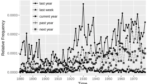
Another aspect that is noticeable in the results is that various temporal expressions appear in the list of features highly correlated with ‘last year’. This suggests that temporal expressions in general increased in usage over time with respect to this genre. Figure 7 shows a few of the expressions from table 1. All seem to increase
Figure 6: News corpus: relative frequency of items with change points around 1915-16 and 1945-46.
● ● ● ● ● ●● ● ●●●●● ●● ● ● ● ● ●● ● ● ●● ● ● ● ● ●●● ● ● ●● ● ● ● ● ● ● ● ● ●● ● ● ● ● ● ● ● ● ● ● ● ● ● ● ●●●●● ● ●●●●●● ● ●● ● ●● ● ● ● ● ● ● ● ●● ●● ● ● ●●● ● ● ●●●● 0.00000 0.00005 0.00010
1880 1890 1900 1910 1920 1930 1940 1950 1960 1970
Time
Relativ
e Frequency
● stock market first quarter
preferred stock
third quarter
[image:7.612.57.303.131.275.2]financial position
Figure 7: News corpus: relative frequency of temporal ex-pressions. ● ● ●● ● ● ● ● ● ● ● ● ● ● ● ● ●● ● ● ● ● ● ●● ● ● ● ● ● ● ● ● ● ● ● ● ● ●● ● ●● ● ● ● ● ● ● ● ● ● ● ● ● ● ● ● ● ● ● ●●● ● ● ● ● ●● ● ●● ● ● ● ● ● ● ● ● ● ●● ● ● ● ● ● ● ● ● ● ● ● ● ● ● ● ● 0.0000 0.0001 0.0002 0.0003
1880 1890 1900 1910 1920 1930 1940 1950 1960 1970
Time
Relativ
e Frequency
● last year
last week
current year
past year
next year
in frequency over time. However, correlation analysis might be a little volatile in that smaller spans of the entire period are not representative of the overall correlation. For this reason, we seek to validate our results further, which will be done in the next section.
6.2
Validation of Results
As the final part of this analysis, we seek to further validate our results. One part of this is to see whether this effect also exists in less changeable genre, such asfiction. Thus, we repeat the exact same experiment, but using thefictioncorpus as a basis rather than the newscorpus. We first estimate possible change points on the basis of the new corpus. Interestingly, the change point for ‘last year’ in the fiction genre happens earlier, around 1917. There seems to be a lot less variety in adjective-noun combinations as the partially constant features over 1918-1928 only add up to 27. Of these 27, only 9 are positively correlated to ‘last year’ based on a span of± 15 around their individual change point.
[image:7.612.55.302.337.478.2]However, onlygood evening,little girl,good night,good timeand very wellare actually positively correlated with ‘last year’ over an
Figure 8: Fiction corpus: relative frequency of highest‘last year’correlated features in the fiction genre.
●●●● ● ●● ● ● ●● ●● ●●● ● ● ●●●●●● ● ●●● ● ●● ●● ● ● ●●● ● ●● ● ●● ● ● ● ● ● ●● ● ●● ● ●●● ● ●● ● ● ●● ●● ● ●●●● ●●●● ● ● ●● ● ● ●● ●● ● ●● ● ●● ● ●● ●●● ● ● 0.00000 0.00005 0.00010 0.00015
1880 1890 1900 1910 1920 1930 1940 1950 1960 1970
Time
Relativ
e Frequency
● last year good evening
little girl
good night
good time
interval of±15 years around its own change point, with the highest correlation being around 0.4. Figure 8 shows them side-by-side with ‘last year’. This suggests that the temporal aspect has not grown as much in importance in this genre and is less closely linked to adjective-noun types as it seems to be the case in thenewsdomain.
In order to validate this in thenewsdata, we consider actual language samples for co-occurrence of items highly correlated with ‘last year’. We randomly extract sentences containing ‘last year’ and observe what concepts co-occur in the same sentences. We take ten samples each from before 1923 (1910-1920), immediately after (1924-1934) and again at a later stage (1950-1960).
Table 2 shows salient concepts occurring in the same sentence as ‘last year’ for all three time periods. The number in bracket indicates in how many sentences of the ten selected ones the term occurred. The terms occurring in the first time span are mostly related to elections and governments with some more general political topics, such ascompanyandwagesentering into it as well. The second time span set around the change in ‘last year’ seems to contain almost exclusively stock exchange related news items. The final period, set after the end of WWII contains very mixed samples from sports, to international politics, companies and space programs. Although extracting a few random samples from a large set of texts cannot provide very fixed conclusions, these results seem to support our earlier findings of a strong correlation between stock exchange related items and the temporal expression ‘last year’ during a particular time period, where this seems to have dominated the news. In order to see to what extent this effect generalizes to other temporal expressions, we need to analyze these separately.
7
DISCUSSION
We have reported an exploratory analysis to investigate the re-lationship between temporal expressions, such as ‘last year’ and temporally less stable word expressions that appear and disap-pear over time. We hypothesized that these fluctuating words that are more strongly connected to current events would somewhat influence the rise in frequency of more stable concepts, such as
Table 2: News corpus: salient words occurring with ‘last year’ in 10 randomly selected sentences for each of the time periods: 1910-1920, 1924-1934, 1950-1960.
News corpus salient words occurring with ‘last year’
1910-1920
(primary) election(2), party(2), board of education(2), mexican bullets (1), company (3),
director(s)(2), railroad(1), wages(1), shareholders(1), submarine(1), national committee(1)
1924-1934
adjustment bond(1), common stock(2), stock (dividend)(2), (cash) investment (2), congress (1), sales(1), share(1),
corporation(1), net profit(1), minor purchases(1), liquidation(1), dividend rate(1), president(1), preferred dividends(1)
1950-1960
tournament(1), basketball coach(1), chicago medical society(1), tax bill(1), (space) administration(2), international agreement(1),
wage(1), arbitration(1), net income(1), auto companies(1), production schedules(1), national aeronautics(1), russians pioneer(1)
temporal expressions. Our results suggest that there might indeed be a connection between ‘last year’ and clusters of words linked to historical events, such as the stock marked crash. However, while stock market related words are only constant and very frequent for a limited time frame, ‘last year’ and other temporal expressions remain frequent. We believe that this could be due to temporal aspect in news language having become more important after 1923, having gathered momentum through events, such as the stock mar-ket crash and then remained to stay. Our parallel analysis of fiction data at the same time seems to confirm this insofar as this effect is not found with the same strength in fiction data. Based on our language sample analysis that appears to support our change point and correlation analysis, ‘last year’ is continued to be used in vari-ous different concepts, possibly more varied than before 1923. Our analysis using change points adds to a simpler relative frequency detection approach by considering the uncertainties associated with our predictions. Although without having conducted a semantic change analysis, we cannot be entirely certain that this change is not caused by a shift in semantics, however, the possible semantic space of temporal expressions could be seen as more limited than that for regular common nouns or adjectives. In fact, these temporal expressions might semantically be closer to function types than to content types, in spite of belonging to the latter word class. In a sense, temporal adverbs are similar to prepositions, only anchored in time rather than in space and consequently there might be less room for reinterpretation of their meaning.
Our results also need validation from historians, especially with respect to events in 1923 that could have caused temporal expres-sions to become more frequent. The type of analysis we have done here shows changes in words’ relative frequency patterns that could reflect political or cultural changes. In this, we are at the mercy of the sampling of our newspaper corpus that although balanced over different sources is not impervious to other external factors that could influence the language samples. For instance, by the mid-1920s, the businessman William Randolph Hearst had acquired 28 newspapers, that consequently have been subject to same edi-torial decisions, distorting our perception of what language was representative for that time.
8
CONCLUSION AND FUTURE WORK
In essence, this work has been exploratory trying to connect groups of words that might not occur close to each other in space making their relatedness less tangible. Although, additional work is needed to further support our findings, our results tentatively suggest that
words or expressions that are stable in occurrence, might be rather volatile with respect to their relative frequency distribution. As temporal expressions have fewer semantic associations, they might depend more strongly on features that do.
The results we have obtained are tentative and in order to claim an increase of temporal expressions possibly related to certain historical events, one needs to show this effect to hold for other temporal expressions as well as exclude any possible semantic shift. We also need validation from historians to interpret and relate our results to historical and cultural changes in or around 1923. Partic-ular language usage and change therein can reflect shifts in society and general opinion, adding a more subtle basis for interpretation of past events.
Acknowledgement
We would like to thank our anonymous reviewers for their helpful suggestions on how to improve the earlier version of this paper. This research is supported by Science Foundation Ireland (SFI) through the CNGL Programme (Grant 12/CE/I2267 and 13/RC/2106) in the ADAPT Centre (www.adaptcentre.ie)
REFERENCES
[1] Joan Bybee and Sandra Thompson. 1997. Three frequency effects in syntax. In
Annual Meeting of the Berkeley Linguistics Society, Vol. 23.
[2] Walter Daelemans. 2013. Explanation in computational stylometry. In
Computa-tional Linguistics and Intelligent Text Processing. Springer, 451–462.
[3] Mark Davies. 2010. The Corpus of Historical American English: 400 million words, 1810-2009.http://corpus. byu. edu/coha/.24 (2010), 2011. (last verified: 24.08.2015).
[4] William L Hamilton, Jure Leskovec, and Dan Jurafsky. 2016. Cultural Shift or Linguistic Drift? Comparing Two Computational Measures of Semantic Change.
InEmpirical Methods in Natural Language Processing (EMNLP).
[5] Nicholas A James, Arun Kejariwal, and David S Matteson. 2016. Leveraging cloud data to mitigate user experience from Breaking Bad. InBig Data (Big Data), 2016
IEEE International Conference on. IEEE, 3499–3508.
[6] Nicholas A James and David S Matteson. 2013. ecp: An R package for non-parametric multiple change point analysis of multivariate data.arXiv preprint
arXiv:1309.3295(2013).
[7] Vivek Kulkarni, Rami Al-Rfou, Bryan Perozzi, and Steven Skiena. 2015. Sta-tistically Significant Detection of Linguistic Change. InProceedings of the 24th
International Conference on World Wide Web (WWW ’15). International World
Wide Web Conferences Steering Committee, Republic and Canton of Geneva, Switzerland, 625–635.https://doi.org/10.1145/2736277.2741627
[8] Meik Michalke. 2014.koRpus: An R Package for Text Analysis. http://reaktanz.de/ ?c=hacking&s=koRpus (Version 0.05-4).
[9] Alex Riba and Josep Ginebra. 2006. Diversity of vocabulary and homogeneity of literary style.Journal of Applied Statistics33, 7 (2006), 729–741.
[10] Helmut Schmid. 1994. Probabilistic part-of-speech tagging using decision trees.
InProceedings of international conference on new methods in language processing,
Vol. 12. Manchester, UK, 44–49.