Abstract—In this paper, we propose the fourth stage of the inverse polynomial scheme for the numerical solution of initial value problems of ordinary differential equations. Binomial expansion and Taylor’s series method are used towards the derivation of the scheme. We further study the analysis properties to show the efficiency of the method. Numerical experiments are carried out and the results are compared with the theoretical solution and some existing methods to show that it is adequate, effective and computationally time friendly.
Index Terms— inverse polynomial, initial value problem, ordinary differential equations, consistency, stability, convergence.
I. INTRODUCTION
n science and engineering, modeling a system frequently amounts to solving an initial value problem. In this context, the differential equation is an evolution equation specifying how, given initial conditions, the system will evolve with time. Turning the rules that govern the evolution of a quantity into a differential equation is called modeling [2].
Numerical method is a substantial aspect in solving initial value problems in ordinary differential equations where the problems cannot be solved or difficult to obtain analytically. The numerical solutions of first order initial value problems have caught much attention recently; a new numerical scheme for the solution of initial value problems in ordinary differential equations was developed [10]. An integrator was also developed in [11] by representing the theoretical solution to initial value problems by an interpolating function which maybe linear or nonlinear.
There is a technique [20] for comparing numerical methods that have been designed to solve stiff systems of ordinary differential equations; the technique was applied to five methods of which three turn out to be quite good. However, each of the three has a weakness of its own, which can be identified with particular problem characteristics. Wavelets was used in solving the first order ordinary differential equations which are either stiff or non-stiff [3]. It is worth mentioning that [1] works on the method for the numerical solution of the Painlevé equations (equations
Manuscript received September 01, 2015; revised May 4, 2017. O. E. Abolarin is with the Department of Mathematics, Federal University Oye-Ekiti, Ekiti State, Nigeria. (Corresponding Author; Phone: +2348038584643; E-mail address: [email protected]) S. W. Akingbade is with the Department of Mathematics, Federal University Oye-Ekiti, Ekiti State, Nigeria.
(E-mail address: [email protected]).
having singularities at points where the solution takes certain finite values). Researchers also worked on some other forms of equations like the integro-differential equations [15] and the integral equations where the Petrov-Galerkin method is employed for the numerical solution of stochastic volterra integral equations [4].
Other notable works are [6], [7], [8], [13], [16], and [19] to mention a few.
In this paper, we developed a numerical integrator capable of solving equations of the form
0 0) ( ); ,
(x y y x y
f
y (1) The integrator is developed by representing the theoretical solution ‘
y
(
x
)
’ to (1) by an interpolating function.In [14], the effectiveness of the first stage, second stage of the inverse polynomial method to solving ordinary differential equations with singularities was shown using a different integrator and [18] worked on the third stage of the method and analyzed its analysis properties; the local truncation error and the order were also determined towards its implementation.
II.
PRELIMINARIESIn this section, we present some useful existing concept and works.
Definition II.1. The conventional one-step numerical integrator for initial value problem (1) is generally described according to [12] as
) ; , (
1 y h x y h
yn n
n n (2)Examples of such method are Euler’s method and Runge-Kutta’s method.
Definition II.2. Truncation error is the error committed when the higher terms of the power series are ignored. Such errors are essentially algorithmic errors and we can predict the extent of the error that will occur in the method.
Definition II.3. An algorithm is said to be numerically stable if an error whatever the cause does not grow much larger during calculation. This happens if the problem is well posed, that is, the solution changes by only a small amount if the problem data are changed by small amounts.
Definition II.4. The simplest methods of order ‘P’ are always based on the Taylor series expansion of the solution ‘y(x)’ of the IVP (1) as in [9]. If we assume ‘yp1(x)’ to
Derivation and Application of Fourth Stage
Inverse Polynomial Scheme to Initial Value
Problems
O. E. Abolarin and S. W. Akingbade
I
IAENG International Journal of Applied Mathematics, 47:4, IJAM_47_4_14
be continuous on the closed interval [a, b], then the Taylor’s formula is given by
. )] ( )! 1 ( ) ( ! ... ) ( ! 2 ) ( [ ) ( ) ( )! 1 ( ) ( ! ... ) ( ! 2 ) ( ) ( ) ( ) ( 1 1 1 1 1 1 2 1 n n n n p p p p n n n n p p p p n n n n n x x where y p h x y p h x y h x y h x y y p h x y p h x y h x y h x y h x y x y
(3)The continuity of ‘ 1( ) x
yp ’ implies that it is bounded on
[a, b] and therefore,
). ( 0 )! 1 ( ) ( 1 1 1 p p n p h p h
y
(4)We introduce (4) in (3),
) ( )] ( ! ... ! 2 ) ( ) ( [ ) ( 1 1 p n p p n n
n y x Oh
p h x y h x y h x y Hence, ) ( )] , ( ! ... )) ( , ( 2 )) ( , ( [ ) ( ) ( 1 ) 1 ( 1 1 p n n p p n n n n n n h O y x f p h x y x f h x y x f h x y x y (5)
Equation (5) is called the Taylor Series Method of order P. In this work, we denote the Taylor’s series method of order 4 as TSM-4.
Definition II.5. Runge-Kutta Method (RK4) is a technique for approximating the solution of ordinary differential equations. It was developed by two mathematicians Carl Runge and Withen Kutta around 1900.
Runge-Kutta method is popular because of its efficient used in most computer programs for differential equations. The most widely used Runge-Kutta scheme is the fourth order scheme RK4 based on Simpson’s rule [17].
( 2 2 )
6 1 2 3 4
1 k k k k
h y
yn n (6)
) , ( ) 2 , 2 1 ( ) 2 , 2 1 ( ) , ( 3 4 2 3 1 2 1 hk y h x f k k h y h x f k k h y h x f k y x f k where n n n n n n n n
III. FOURTHSTAGEINVERSEPOLYNOMIAL SCHEME
Let the numerical approximation ‘ 1
n
y ’ evaluated at
1
x
nx
to exact solution ‘ ( )1
n
x
y ’ to the first order
ordinary differential equation be represented as
1 0 1
kj
j n j n
n
y
a
x
y
(7)The parameters
a
js
'
are to be determined from the non-linear equations that will be generated by considering the following steps:1. For the fourth order, k=4, and setting
a
0
1
4
14 3 3 2 2 1
1 1 ( )
n n n n n
n y ax a x a x a x
y (8)
2. Obtain the Binomial Expansion of (8)
4 4 4 3 3 2 2 1 3 4 4 3 3 2 2 1 2 4 4 3 3 2 2 1 4 4 3 3 2 2 1 1 ) ( ! 4 ) 4 )( 3 )( 2 )( 1 ( ) ( ! 3 ) 3 )( 2 )( 1 ( ) ( ! 2 ) 2 )( 1 ( ) )( 1 ( 1 n n n n n n n n n n n n n n n n n n x a x a x a x a x a x a x a x a x a x a x a x a x a x a x a x a y y
3. Express the left hand side of (8) in terms of its Taylor's series expansion
! 4 ! 3 ! 2 ) 4 ( 4 3 2 n n n n n n y h y h y h y h y h
y
4. Insert the obtained equations from steps 2 and 3 above into (8) and expand
n n n n n n n n n n n n n n y x a a a a a a a y x a a a a y x a a y x a y y h y h y h y h y 4 2 2 1 4 1 4 2 2 3 1 3 3 3 1 2 1 2 2 2 1 ) 4 ( 4 3 2 ) 3 2 ( ) 2 ( ) ( ! 4 ! 3 ! 2 1
5. We make the expression above agrees term by term for each parameter.
n n
n a x y
y
h 1
n n n y x y h
a1 (9)
n n n y x a a y h 2 2 2 1 2 ) ( !
2
Solve for
a
2by substituting (9) 2 2 2 2 2 2 2 ) ( 2 n n n n n y x y y h y ha (10)
n n
n aa a a x y
y
h 3 3
1 3 2 1 3 ) 2 ( !
3
Using (9) and (10),
3 3
3 3 2 2 2 2 2 3 3 3 ) ( 2 ) ( 2 2
6 n n
n n n n n n n n n n n n y x y h y x y y h y h y x y h y x y h a 3 3 3 3 3 2 3 3 6 ) ( 6 6 n n n n n n n n y x y h y y y h y y h a
(11)
n n
n aa a a a a a x y
y h 4 2 2 1 4 1 4 2 2 3 1 ) 4 ( 4 ) 3 2 ( !
4
n n n
y
x
y
h
a
a
a
a
a
a
a
4 ) 4 ( 4 2 2 1 4 1 2 2 3 1 4!
4
3
2
We express each term of
a
4 above in relation to (9), (10), and (11)IAENG International Journal of Applied Mathematics, 47:4, IJAM_47_4_14
4 4 4 4 4 4 2 4 4 4 4 4 4 4 2 4 3 1 ) ( 2 ) ( 2 ) ( 4 3 2 n n n n n n n n n n n n n n n n y x y h y x y y y h y x y h y x y y y h a
a
4 4 2 2 4 4 4 2 4 4 4 4 4 2 2 4 ) ( ) ( ) ( n n n n n n n n n n n n y x y y h y x y y y h y x y h
a
4 4 4 4 4 4 2 4 2 2 1 4 1 ) ( 2 2 ) ( 3 3 n n n n n n n n y x y h y x y y y h a a
a
Finally, n n n n n n n n n n n n n y x y y h y y h y y y h y y y h y h
a 4 4
2 2 4 ) 4 ( 3 4 2 4 2 4 4 4 4 24 ) ( ) ( 6 8 ) ( 36 ) ( 24
(12)
By using (9), (10), (11), and (12) in (8), we have the fourth stage Inverse Polynomial:
1 ) 4 ( 3 4 2 2 4 2 4 2 4 3 3 4 4 3 3 2 3 3 2 2 2 2 3 4 5 ) ( ) ( 6 ) ( 36 8 4 ) ( 24 ) ( 24 24 12 ) ( 24 24 24 24 n n n n n n n n n n n n n n n n n n n n n n n n n n y y h y y h y y y h y y y h y y h y h y y h y y y h y y h y y h y hy y y (13)
Equation (13) is the Fourth Stage Inverse Polynomial Scheme (New Method).
IV. ANALYSISOFTHEBASICPROPERTIESOFTHE FOURTHSTAGESCHEME
A. Consistency
A numerical scheme with an increment function ‘(xn,yn;h)’ is said to be consistent with the initial value
problem (1) if
x y
f h yxn, n; ) ,
(
when h=0.From (2)
yn1yn h
(xn,yn;h) (14)( , ; )
,
1 x y h
h y y n n n
n
In light of this, with respect to the scheme,
nn n n n n n n n n n n n n n n n n n n n n n n n n n n n y y y h y y h y y y h y y y h y y h y h y y h y y y h y y h y y h y hy y y y y 1 ) 4 ( 3 4 2 2 4 2 4 2 4 3 3 4 4 3 3 2 3 3 2 2 2 2 3 4 5 1 ) '' ( ) ( 6 '' ) ( 36 8 4 ) ( 24 ) ( 24 '' 24 '' 12 ) ( 24 24 24 24
4 2 2 2 2 3 (4)
4 2 3 3 2 2 2 3 4 ) 4 ( 4 2 3 3 2 2 4 4 2 3 2 3 2 3 2 4 5 5 ) ( 6 8 ) ( 36 ) ( 24 ) ( 6 6 4 ) ( 2 12 24 24 ) ( 6 8 ) ( 36 ) ( 24 [ ] ) ( 6 6 [ 4 ) ( 2 12 24 24 24 n n n n n n n n n n n n n n n n n n n n n n n n n n n n n n n n n n n n n n n n n n n n n n n n n n n n y y y y y y y y y y y h y y y y y y y h y y y y h y hy y y y y y y y y y y y y y h y y y y y y y h y y y y h y hy y y h y yn 1 n
4 2 2 2 2 3 (4)
4 2 3 3 2 2 2 3 4 ) 4 ( 4 2 3 3 2 2 4 3 2 3 2 2 3 4 ) ( 6 8 ) ( 36 ) ( 24 ) ( 6 6 4 ) ( 2 12 24 24 ) ( 6 8 ) ( 36 ) ( 24 [ ] ) ( 6 6 [ 4 ) ( 2 12 24 n n n n n n n n n n n n n n n n n n n n n n n n n n n n n n n n n n n n n n n n n n n n n n n n n n y y y y y y y y y y y h y y y y y y y h y y y y h y hy y y y y y y y y y y y y y h y y y y y y y h y y y y h y y h
4 2 2 2 2 3 (4)
4 2 3 3 2 2 2 3 4 4 3 2 3 2 2 4 4 2 3 2 3 2 3 2 4 1 ) ( 6 8 ) ( 36 ) ( 24 ) ( 6 6 4 ) ( 2 12 24 24 ) ( 6 8 ) ( 36 ) ( 24 ) ( 6 6 4 ) ( 2 12 24 n n n n n n n n n n n n n n n n n n n n n n n n n iv n n n n n n n n n n n n n n n n n n n n n n n n n n y y y y y y y y y y y h y y y y y y y h y y y y h y y h y y y y y y y y y y y y y h y y y y y y y h y y y y h y y h h y y
4 2 2 2 2 3 (4)
4 2 3 2 2 2 2 3 4 4 3 2 3 2 2 4 3 2 3 2 2 2 3 4 1 ) ( 6 8 ) ( 36 ) ( 24 ) ( 6 6 4 ) ( 2 12 24 24 ) ( 6 8 ) ( 36 ) ( 24 ) ( 6 6 4 ) ( 2 12 24 n n n n n n n n n n n n n n n n n n n n n n n n n iv n n n n n n n n n n n n n n n n n n n n n n n n n n y y y y y y y y y y y h y y y y y y y h y y y y h y y h y y y y y y y y y y y y y h y y y y y y y h y y y hy y y h y y
4 2 2 2 2 3 (4)
4 2 3 2 2 2 2 3 4 4 2 3 3 2 2 4 3 2 3 2 2 2 3 4 1 ) ( 6 8 ) ( 36 ) ( 24 ) ( 6 6 4 ) ( 2 12 24 24 ) ( 6 8 ) ( 36 ) ( 24 ) ( 6 6 4 ) ( 2 12 24 n n n n n n n n n n n n n n n n n n n n n n n n n iv n n n n n n n n n n n n n n n n n n n n n n n n n n y y y y y y y y y y y h y y y y y y y h y y y y h y hy y y y y y y y y y y y y y h y y y y y y y h y y y hy y y h y y
Taking the limit as h approaches zero,
n n n y h y
y 1
(15)
B. Stability
One-step scheme is said to be stable if for any initial error
0
e
, there exist a constant M andh
0>0 such that when the general one-step scheme is applied to initial value problems with step size (0, ),0
h
h the ultimate error
e
n satisfies the following inequalities
0 Me en and 0M 1
Using the general form, 1 0 1
kj j h n j h n h
n y a x
y (16)
The theoretical solution y(x) is given as
h n k j j h n j h n h
n y x a x T
x y
1 0 1) ( )( (17)
h n k j j h n j h n k j j h n j h n h n h
n
y
y
x
a
x
y
a
x
T
x
y
1 0 1 1 0 1)
(
)
(
h n k j j h n j h n hn
e
a
x
T
e
1 01 (18)
We take the absolute value of both sides,
h n k j j h n j h n h
n e a x T
e
1 0 1We assume that
k j h n j jx a Q 0 (19) Then,IAENG International Journal of Applied Mathematics, 47:4, IJAM_47_4_14
1
0 1
0
kj
j h n j k
j
j h n
j
x
a
x
a
M
Q
x
a
k
j
j h n
j
11
0
(20)
h n h n h
n Me T
e 1 (21) Let
E
nh
sup(
e
nh)
and Tsup(Tnh)Similarly,
sup(
)
1
1
h
n hn
e
E
with 0nWe then have in the form
T
ME
E
nh
nh1
(22) For h=1,T ME
En1 n
For h=2,
T
ME
E
n2
n1
T MT E
M
T T ME M
n n
2
) (
T MT E
M
En n
2 2
For h=3,
T
ME
E
n3
n2
M(M2EnMTT)T
T MT T M E M
En n
2 3
3
The general form is
0
r r n
k h
n M E M T
E (23)
0
r r n
k h n k
n E M E M T
e
Since M<1 and as n,Enh 0
This shows that the method is stable and also convergent. C. Convergence
The necessary and sufficient conditions for a numerical method to be convergent are stability and consistency. Since these conditions are satisfied, we can conclude that the proposed method is Convergent.
More of stability, consistency and convergence shall be discussed in the next section by considering some test problems.
V. NUMERICALRESULTSANDINTERPRETATIONS. A. Test problems
We require that the first, second,
third and fourth derivatives with respect to
‘x’ of the interpolating function, respectively coincide with the differential equation as well as its first, second, third and fourth derivatives with respect to x at
x
n. In other words, we require that,3 )
4 (
2
) (
) (
) (
) (
n n
n n
n n
n n
f x y
f x y
f x y
f x y
Now for
n x x
h n 0 , (24)
We generate iterations to determine ‘
y
n’ at each value of ‘xn’.We shall compare our results with the Taylor’s series method of order P=4 (TSM-4), Runge-kutta of order 4 (RK4) and the exact solution of each of the initial value problems in order to show the effectiveness of the new method. We consider the following examples:
Example 1
The logistics growth modelled by the differential equation
) 1 (
m p kp dt
dp
for some positive constants
k
andm
We now take the IVP(xt):5 . 0 ) 0 ( ); 1
(
y y y
y (a)
1 . 0 h
The exact solution is given as t
e t
y
5 . 0 5 . 0
5 . 0 )
(
Table I
Results of Example 1
t
New Method Exact solution Error 0.0 0.500000000 0.500000000 0.000000000 0.1 0.524979165 0.524979187 0.000000022 0.2 0.549833952 0.549833997 0.000000045 0.3 0.574442450 0.574442516 0.000000066 0.4 0.598687573 0.598687660 0.000000087 0.5 0.622459225 0.622459331 0.000000106 0.6 0.645656182 0.645656306 0.000000124 0.7 0.668187632 0.668187772 0.000000140 0.8 0.689974326 0.689974481 0.000000157 0.9 0.710949335 0.710949502 0.000000167 1.0 0.731058400 0.731058578 0.000000178Example 2
The non-linear initial value problem as in [5]
1 ) 0 ( , 1 ) 0 ( ; 0 )
( 2
y y y
y (b)
1 . 0
h , 1.0
n
x
This can be reduced to the desired order by the method of reduction of order. The exact solution is then given as
1 1 ) (
x x y
IAENG International Journal of Applied Mathematics, 47:4, IJAM_47_4_14
Table II
Results of Example 2
x
TSM-4 RK4 New Method0.0 1.000000000 1.000000000 1.000000000 0.1 0.909033333 0.909091186 0.909090909 0.2 0.833290126 0.833333729 0.833333333 0.3 0.769197044 0.769231206 0.769230769 0.4 0.714258558 0.714286154 0.714285714 0.5 0.666644250 0.66666709 0.666666667 0.6 0.624981120 0.624980325 0.625000000 0.7 0.588219131 0.588217885 0.588235294 0.8 0.555541530 0.555540041 0.555555556 0.9 0.526303480 0.525828299 0.526315790 1.0 0.499989092 0.499560026 0.500000000 The exact solution is given as follows
Table III
Exact Solution to (b)
x
Exact solution 0.0 1.000000000 0.1 0.909090909 0.2 0.833333333 0.3 0.769230769 0.4 0.714285714 0.5 0.666666667 0.6 0.625000000 0.7 0.588235294 0.8 0.555555556 0.9 0.526315790 1.0 0.500000000 Table IVError Analysis from the Results of Example 2
x
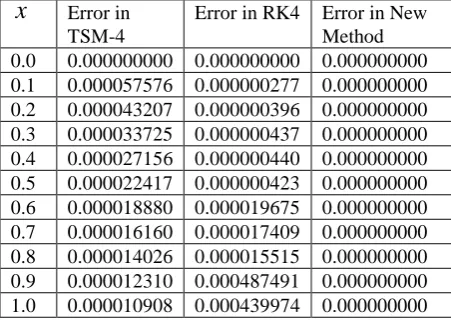
Error in TSM-4Error in RK4 Error in New Method 0.0 0.000000000 0.000000000 0.000000000 0.1 0.000057576 0.000000277 0.000000000 0.2 0.000043207 0.000000396 0.000000000 0.3 0.000033725 0.000000437 0.000000000 0.4 0.000027156 0.000000440 0.000000000 0.5 0.000022417 0.000000423 0.000000000 0.6 0.000018880 0.000019675 0.000000000 0.7 0.000016160 0.000017409 0.000000000 0.8 0.000014026 0.000015515 0.000000000 0.9 0.000012310 0.000487491 0.000000000 1.0 0.000010908 0.000439974 0.000000000
Example 3
We consider the special initial value problem in ordinary differential equation of the form
1 2; (0)1, 0.01 h
y y
y , 0x0.04 (c)
The exact result is given as
1 0
); 4 tan( )
(x x x
[image:5.595.304.413.288.441.2]y
Table V
Results of Example 3
x
TSM-4 RK4 New Method0.00 1.0000000 1.0000000 1.0000000 0.01 1.0202027 1.0202027 1.0202027 0.02 1.0408219 1.0408219 1.0408219 0.03 1.0618748 1.0618748 1.0618748 0.04 1.0833797 1.0833797 1.0833797 0.05 1.1053556 1.1053556 1.1053556 0.06 1.1278228 1.1278228 1.1278228 0.07 1.1508026 1.1508026 1.1508026 0.08 1.1743174 1.1743174 1.1743174 0.09 1.1983911 1.1983911 1.1983911 0.10 1.2230489 1.2230489 1.2230489 The exact solution is given as follows
Table VI
Exact Solution to (c)
x
Exact Solution 0.00 1.0000000 0.01 1.0202027 0.02 1.0408219 0.03 1.0618748 0.04 1.0833797 0.05 1.1053556 0.06 1.1278228 0.07 1.1508026 0.08 1.1743174 0.09 1.1983911 0.10 1.2230489B. Interpretation of results
We have implemented the fourth stage of the Inverse Polynomial Scheme which has an advantage over all previously proposed methods of the same order as it is seen in Table II when it was compared with Runge-Kutta method of order 4 (RK4) and the Taylor’s series method P=4 (TSM-4). Table IV showed the analysis of error in each of the methods. In Table I, the new method is well behaved when compared with the exact solution. This makes it to be more accurate and reliable.
Example 3 is a special initial value problem which is unbounded or undefined at ‘
4
x ’
So, the new method compared favourably with the existing methods and the exact method when called upon to solve this form of initial value problem as shown above in Table V.
From all the examples, we can see that the issue of stability and consistency of the new scheme is well demonstrated and thereby showing a measure of convergence towards the exact solution.
ACKNOWLEDGMENT
The authors are grateful to the reviewers for their helpful suggestions and valuable comments towards the improvement of the paper.
IAENG International Journal of Applied Mathematics, 47:4, IJAM_47_4_14
[image:5.595.61.287.486.646.2]REFERENCES
[1] A. A. Abramov and L. F. Yukhno, “A method for the numerical solution of Painleve equations,” Journal of Computational mathematicsandmathematicalphysics. vol. 53, no 5, pp. 540-563, 2013.
[2] P. Blanchard, R. L. Devaney and G. R. Hall, Differential equations (4th ed). Boston: Richard Stratton. Retrieved November 5, 2012.
[3] C. H. Hsiao, “Numerical solution of stiffs differential equation via Harr wavelets,” International Journal of Computer Mathematics. vol. 82, pp. 1117-1123, 2005.
[4] F. Hosseini Shekarabi, M. Khodabin and K. Maleknejad, “The Petrov-Galerkin method for numerical solution of stochastic volterra integral equations,” IAENG International Journal of Applied Mathematics. vol. 44, no. 4, pp. 170-176, 2014.
[5] “Reduction of order” CliffsNotes.com. Houghton Mifflin Harcourt,
2014.
[6] E. Hairer and G. Wanner, Solving ordinary differential equations II. Stiff and differential-algebraic problems. Second Ed, Springer-Verlag, 1996,pp. 2-11.
[7] Dingwen Deng and Tingting Pan, “A fourth-order singly diagonally implicit Runge-Kutta method for solving one-dimensional Burgers’ equation,” IAENG International Journal of Applied Mathematics.vol. 45, no. 4, pp. 327-333, 2015.
[8] S. O. Fatunla, Numerical methods for initial value problems in ODEs. Academic Press Inc. UK, 1988, pp. 20-88.
[9] G. F. Corliss and Y. F. Chang, “Solving ODEs using Taylor series”, ACM Transactions on Mathematical Software.pp. 114-144, 1982.
[10] E. A. Ibijola and R. B. Ogunrinde, “On a new numerical scheme for the solution of IVPs in ODEs,” Australian Journal of Basic and Applied Sciences. vol. 4, no. 10, pp. 5277-5282, 2010.
[11] J. Sunday and M. R Odekunle, “A new numerical integrator for the solution of initial value problems in ODEs,” Pacific Journal of Science and Technology.vol. 13, no 1,pp. 221-227, 2012.
[12] J. D. Lambert, Computational methods in ODEs. John Willey and sons, NewYork. 1973, ch 4
[13]P. Kama and E. A. Ibijola, “On a new one step method for numerical solution of ODEs,” International Journal of Computer Mathematics vol. 78, no. 4, pp. 457-467, 2000.
[14] K. O. Okosun, “kth order inverse polynomial methods for the integration of ordinary differential equations with singularities,” An M.Tech Thesis, Industrial Mathematics and Computer department, Federal University of Technology, Akure.Nigeria, 2003.
[15] M. Asgari, “Numerical solution for solving a system of fractional integro-differential equations,” IAENG International Journal of Applied Mathematics.vol. 45, no 2, pp. 85-91, 2015.
[16] L. F. Shampine, Numerical Solutions of ODEs. Chapman & Hall, New York, 1994, pp. 138-159
[17] P. Kaps, P. Rentrop, “Generalized Runge-Kutta methods of order four with step size control for stiff ODEs,” Numerische Mathematik. vol. 33, no 1, pp 55-68, 1979.
[18] R. B. Ogunrinde, “On a new inverse polynomial numerical scheme for the solution of IVPs in ODEs,” International Journal of Mathematical, Computational, Physical, Electrical and Computer Engineering, Waset.vol. 9, no. 2,2015.
[19] A. Wambecq, “Nonlinear methods in solving ODEs,” Journal of computational & applied Mathematics vol. 2, no. 1, pp. 27-33, 2012. [20] W. H. Enright, T. E. Hull, B. Lindberg, “Comparing numerical
methods for stiff systems of ODEs,” BIT Numerical Mathematics. vol. 15, no. 1, pp. 10-48, 1975.