Nonparametric Bayesian Semi-supervised Word Segmentation
Ryo Fujii Ryo Domoto Hakuhodo Inc. R&D Division 5-3-1 Akasaka, Minato-ku, Tokyo
{ryo.b.fujii,ryo.domoto}@hakuhodo.co.jp
Daichi Mochihashi
The Institute of Statistical Mathematics 10-3 Midori-cho, Tachikawa city, Tokyo
[email protected] Abstract
This paper presents a novel hybrid genera-tive/discriminative model of word segmenta-tion based on nonparametric Bayesian meth-ods. Unlike ordinary discriminative word seg-mentation which relies only on labeled data, our semi-supervised model also leverages a huge amounts of unlabeled text to automat-ically learn new “words”, and further con-strains them by using a labeled data to seg-ment non-standard texts such as those found in social networking services.
Specifically, our hybrid model combines a discriminative classifier (CRF; Lafferty et al. (2001) and unsupervised word segmentation (NPYLM; Mochihashi et al. (2009)), with a transparent exchange of information between these two model structures within the semi-supervised framework (JESS-CM; Suzuki and Isozaki (2008)). We confirmed that it can appropriately segment non-standard texts like those in Twitter and Weibo and has nearly state-of-the-art accuracy on standard datasets in Japanese, Chinese, and Thai.
1 Introduction
For any unsegmented language, especially East Asian languages such as Chinese, Japanese and Thai, word segmentation is almost an inevitable first step in natural language processing. In fact, it is be-coming increasingly important lately because of the growing interest in processing user-generated me-dia, such as Twitter and blogs. Texts in such media are often written in a colloquial style that contains many new words and expressions that are not present in any existing dictionaries. Since such words are theoretically infinite in number, we need to lever-age unsupervised learning to automatically identify them in corpora.
For this purpose, ordinary supervised learning is clearly unsatisfactory; even hand-crafted
dictionar-ies will not suffice because functional expressions more complex than simple nouns need to be recog-nized through their relationship with other words in text, which also might be unknown in advance. Pre-vious studies of this issue used character and word information in the framework of supervised learning (Kruengkrai et al., 2009; Sun et al., 2009; Sun and Xu, 2011). However, they
(1) did not explicitly model new words, or
(2) did not give a seamless combination with dis-criminative classifiers (e.g., they just used a threshold to discriminate between known and unknown words).
In contrast, unsupervised word segmentation methods (Goldwater et al., 2006; Mochihashi et al., 2009) use nonparametric Bayesian generative models for word generation to infer the “words” only from observations of raw input strings. These methods work quite well and have been used not only for tokenization but also for machine transla-tion (Nguyen et al., 2010), speech recognitransla-tion (Lee and Glass, 2012; Heymann et al., 2014), and even robotics (Nakamura et al., 2014).
However, from a practical point of view, such purely unsupervised approaches do not suffice. Since they only aim to maximize the probability of the language model on the observed set of strings, they sometimes yield word segmentations that are
ãôO¦·¢{{ã:YÅèQBSUZØ$^|º{{{
VV¤$•GV
^Þ—×&NJOFN!á\$7BñÂ|×b·ö •i•i•°bi| KHËbº·i|äØ®{{{
¹¹péýCPCPü{Öóyy${D1®
A·p7'D.LýÕ<ÝúNzìí
+ˆ$7
Figure 1: Excerpt of Weibo tweets. It contains many “un-known” words such as novel proper nouns, terms from local dialects, etc., that cannot be covered by ordinary la-beled data or dictionaries.
179
different from human standards on low frequency words.
To solve this problem, this paper describes a novel combination of a nonparametric Bayesian gener-ative model (NPYLM; Mochihashi et al. (2009)) and a discriminative classifier (CRF; Lafferty et al. (2001)). This combination is based on a semi-supervised framework called JESS-CM (Suzuki and Isozaki, 2008), and it requires a nontrivial exchange of information between these two models. In this approach, the generative and discriminative models will “teach each other” and yield a novel log-linear model for word segmentation.
Experiments on standard datasets of Chinese, Japanese, and Thai indicate that this hybrid model achieves nearly state-of-the-art accuracy on standard corpora, and, thanks to our nonparametric Bayesian model of infinite vocabulary it can accurately seg-ment non-standard texts like those in Twitter and Weibo (the Chinese equivalent of Twitter) without any human intervention.
This paper is organized as follows. Section 2 in-troduces NPYLM which will be leveraged in the framework of JESS-CM, described in Section 3. Section 4 introduces our model, NPYCRF, and the necessary exchange of information, while Sec-tion 5 is devoted to experiments on datasets in Chi-nese, JapaChi-nese, and Thai. We analyze the results and discuss future directions of research on semi-supervised learning in Section 6 and conclude in Section 7.
2 Unsupervised Word Segmentation
To acquire new words from an observation consist-ing of raw strconsist-ings, a generative model of words can be extremely useful for word segmentation. Goldwater et al. (2006) showed that a bigram hi-erarchical Dirichlet process (HDP) model based on Gibbs sampling can effectively find “words” in small corpora. In extending this work, Mochihashi et al. (2009) proposed a nested Pitman-Yor language model (NPYLM), a hierarchical Bayesian language model, where charactern-grams (actually,∞-grams
(Mochihashi and Sumita, 2008)) are embedded in word n-grams, and an efficient dynamic
program-ming algorithm for inference exists. Conceptually, NPYLM posits that an infinite number of spellings,
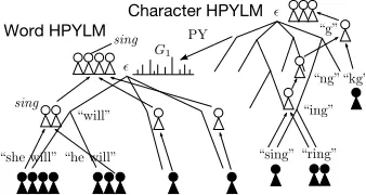
[image:2.612.340.509.55.145.2]Character HPYLM Word HPYLM
Figure 2: The structure of NPYLM by a Chinese Restau-rant Process representation (replicated from Mochihashi et al. (2009)). The word and character HPYLM are drawn as suffix trees; the character HPYLM is a base measure for the word HPYLM, and the two are learned as a single model. Each black customer is a count in HPYLM, and a white customer is a latent proxy customer initiated from each black customer: see Teh (2006) for details.
i.e., “words”, are probabilistically generated from charactern-grams, and a word unigram is drawn
us-ing the charactern-grams as the base measure. Then
bigram and trigram distributions are hierarchically generated and the final string is yielded from the “word”n-grams, as shown in Figure 2.
Practically, NPYLM can be considered as a hi-erarchical smoothing of the Bayesian n-gram
lan-guage model, HPYLM (Teh, 2006). In HPYLM, the predictive distribution of a wordw=wtgiven a
his-toryh=wt−(n−1)· · ·wt−1 is expressed as
p(w|h) = c(w|h)−d·thw θ+c(h) +
θ+d·th· θ+c(h) ·p(w|h
′) (1)
wherec(w|h)denotes the observed counts,θand d
are model parameters, andthwandth·=Pwthware
latent variables estimated in the model.
The probability of w given h is
recur-sively interpolated using a shorter history
h′ = wt−(n−2)· · ·wt−1. If h is already empty
at the unigram level, NPYLM employs a back-off distribution using charactern-grams forp(w|h′):
p0(w) =p(c1· · ·ck) (2) =Qki=1p(ci|c1· · ·ci−1). (3)
In this way, NPYLM can assign appropriate prob-abilities to every possible sequence of segmenta-tion and learn the word and character n-grams at the same time by using a single generative model (Mochihashi et al., 2009).
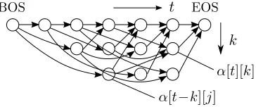
node corresponds to an inside probability α[t][k]1
that equals the probability of a substring ct1 = c1· · ·ct with the last k characters ctt−k+1 being a
word. This inside probability can be computed re-cursively as follows:
α[t][k] = L
X
j=1
p(ctt−k+1|ctt−k−j+1−k )·α[t−k][j] (4)
Here,1≤L≤t−kis the maximum allowed length of
a word. With these inside probabilities, we can make use of Markov Chain Monte Carlo (MCMC) method with an efficient forward filtering-backward sam-pling algorithm (Scott, 2002), namely a “stochas-tic Viterbi” algorithm to iteratively sample “words” from raw strings in a completely unsupervised fash-ion, while avoiding local minima.
[image:3.612.324.526.53.134.2]Problems and Beyond Unsupervised word seg-mentation with NPYLM works surprisingly well for many languages (Mochihashi et al., 2009); however, it has certain issues. First, since it optimizes the performance of the language model, its segmenta-tion does not always conform to human standards and depends on subtle modeling decisions. For ex-ample, NPYLM often separates inflectional suffixes in Japanese like “る” in “見–る” from the rest of the verb, when it is actually a part of the verb it-self. Second, it can produce deficient segmenta-tions for low-frequency words and the beginning or ending of a string where the available information comes from only one direction. These issues can be alleviated by using na¨ıve semi-supervised learn-ing method (Mochihashi et al., 2009) that simply
Figure 3: Semi-Markov model representation of NPYLM (simplest case of segment length≤3). Each node corre-sponds to a substring ending at timet, and its lengthkis indexed by each row.
[image:3.612.96.278.504.580.2]1While we consider only bigrams in this paper for simplic-ity, the theory can be naturally extended to higher-order n-grams. However, it requires quite a complicated implementa-tion, and the expected gain in performance will not be large, even if we use trigrams (Mochihashi et al., 2009).
Figure 4: Semi-supervised learning of the same model structure (HMM and CRF) with JESS-CM. Discrimina-tive and generaDiscrimina-tive potentials are given relaDiscrimina-tive weights 1 :λ0, and added together in the log probability domain.
addsn-gram counts from supervised segmentations
in advance. However, this solution is not perfect because these supervised counts will eventually be overwhelmed by the unsupervised counts, because the overall objective function remains unsupervised. To resolve this issue, we must resort to an explicit semi-supervised learning framework that combines both discriminative and generative models. We used JESS-CM (Suzuki and Isozaki, 2008), currently the best such framework for this purpose, which we will briefly introduce below.
3 Integration with a Discriminative Model JESS-CM (Joint probability model Embedding style Semi-Supervised Conditional Model) is a semi-supervised learning framework that outperforms other generative and log-linear models (Druck and McCallum, 2010). In JESS-CM, the probability of a label sequenceygiven an input sequencexis
writ-ten as follows:
p(y|x)∝pDISC(y|x; Λ)pGEN(y,x; Θ)λ0 (5)
wherepDISCandpGENare respectively the
discrim-inative and generative models, andΛandΘare their
corresponding parameters. Equation (5) is the prod-uct of the experts, where each expert works as a “constraint” to the other with a relative geometrical interpolation weight1 :λ0. If we takepDISC to be a
log-linear model like CRF (Lafferty et al., 2001):
pDISC(y|x)∝expPKk=1λkfk(y,x)
, (6)
Equation (5) can be also expressed as a log-linear model with a new “feature function”
logpGEN(y,x):
p(y|x)∝expλ0logpGEN(y,x) +PKk=1λkfk(y,x)
Here, the parameterΛ = (λ0, λ1,· · · , λK)includes
the interpolation weightλ0and
F(y,x) = (logpGEN(y,x), f1(y,x),· · · , fK(y,x)).
JESS-CM interleaves the optimization ofΛandΘ
to maximize the objective function
p(Yl, Xu|Xl; Λ,Θ) =p(Yl|Xl; Λ)·p(Xu; Θ) (8)
wherehXl, Yli is the labeled dataset and Xu is the
unlabeled dataset.
Suzuki and Isozaki (2008) conducted semi-supervised learning on a combination of a CRF and an HMM, as shown in Figure 4. Since CRF and HMM have the same Markov model structure, they interpolate two weights
PK
k=1λkfk(yt, yt−1,x) and (9) λ0logpGEN(yt|yt−1,x) (10)
on the corresponding path, altenately
• fixingΘand optimizingΛof CRF onhXl, Yli,
and
• fixingΛand optimizingΘof HMM onXu
until convergence, and thereby iteratively maximiz-ing the two terms in (8).
Through this optimization, pDISC andpGEN will
“teach each other” to make the feature logpGEN
more accurate, and further rectified by pDISC with
respect to the labeled data. Note that the interpo-lation weightλ0is automatically computed through
this process.
4 Connecting Two Worlds: NPYCRF We wish to integrate NPYLM and CRF, applying semi-supervised learning via JESS-CM. Note that Suzuki and Isozaki (2008) implicitly assumed that the discriminative and generative models have the same structure as shown in Figure 4. Since NPYLM is a semi-Markov model as described in Section 2, a na¨ıve approach would be to combine it with a semi-Markov CRF (Sarawagi and Cohen, 2005) as the dis-criminative model.
However, this strategy does not work well for two reasons: First, since a semi-Markov CRF is a model for transitions between segments, it cannot deal with character-level transitions and thus per-forms suboptimally on its own. In fact, our pre-liminary supervised word segmentation experiments showed a F1 measure of around 95%, whereas a
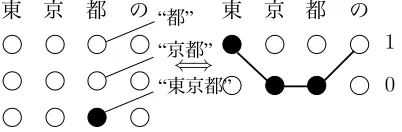
⇐⇒
東 京 都 の “都” 東 京 都 の “京都”
“東京都”
1
[image:4.612.321.522.53.119.2]0
Figure 5: Equivalence of semi-Markov (left) and Markov (right) potentials. The potential of substring “東京都” (Tokyo prefecture) being a word on the left is equivalent to the sum of potentials along the U-shaped path on the right.
character-wise Markov CRF achieves >99%.
Sec-ond, the semi-Markov CRF was originally designed to chunk at most a few words (Sarawagi and Cohen, 2005). However, in word segmentation of Japanese, for example, we often encounter long proper nouns or Katakana sequences that are more than ten char-acters, requiring a huge amount of memory even for a small dataset.
In this paper we instead transparently exchange information between the Markov model (CRF) on characters and the semi-Markov model (NPYLM) on words to perform a semi-supervised learning on different model structures. Called NPYCRF, this unified statistical model makes good use of the dis-criminative model (CRF) from the labeled data and the generative model (NPYLM) from the unlabeled data.
4.1 CRF→NPYLM
To convert from a CRF to NPYLM, we can easily translate Markov potentials into semi-Markov po-tentials as shown in Andrew (2006) for the super-vised learning case.
Consider the situation depicted in Figure 5. Here we can see that the potential of the substring “東京 都” (Tokyo prefecture) in the semi-Markov model (left) corresponds to the sum of the potentials in the Markov model (right) along the path shown in bold. Here, we introduce binary hidden states in the Markov model for each character, similarly to the BI tags used in supervised learning, where state1
repre-sents the beginning of a word and state0represents
a continuation of the word.
Mathematically, we define γ[a, b) as the sum of the potentials along a U-shaped path over an inter-val[a, b)(a < b) as shown in Figure 5, which begins
k j
t t−k+1 t−k
t−k−j+1
[image:5.612.82.284.51.107.2]k j t−k+1t t+1t+j
Figure 6: Substring transitions for marginalization.
Using this notation, the potential that corresponds to
α[t][k] is γ[t−k+ 1, t + 1) covering ct−k+1· · ·ct,
and thus the forward recursion of the inside proba-bilityα[t][k]that incorporates the information from
the CRF can be written as follows, instead of (4):
α[t][k] = L
X
j=1
exphλ0logp(ctt−k+1|ct−kt−k−j+1)
+γ[t−k+1, t+1)i·α[t−k][j]. (11)
Backward sampling can be performed in a similar fashion. In this way, we can incorporate information from the character-wise discriminative model (CRF) into the language model segmentation of NPYLM.
4.2 NPYLM→CRF
On the other hand, translating the information from the semi-Markov to Markov model, i.e., translat-ing a potential from the word-based language model into the character-wise discriminative classifier, is not trivial. However, as we describe below, it is ac-tually possible to do so by extending the technique proposed in Andrew (2006).
Note that for the inference of CRF, from the stan-dard theory of log-linear models we only have to compute its gradient with respect to the expectation of each feature in the current model. This reduces the problem to a computation of the marginal prob-ability of each path, which can be derived within the framework of semi-Markov models as follows:
Semi-Markov feature λ0. Following the line of
argument presented in the Section 4.1, the po-tential with respect to the semi-Markov feature weight λ0 that is associated with the word
transi-tion ctt−−kk−j+1 → ctt−k+1, shown in Figure 6, can
be expressed as an expectation using the standard forward-backward formula:
p(ctt−k+1, ctt−k−j+1−k |s) =α[t−k][j]β[t][k]·
exphλ0logp(ctt−k+1|ctt−−kk−j+1) +γ[t−k+1, t+1)
i
/Z(s) (12) Here,Z(s)is a normalizing constant associated with
each input strings, andβ[t][k]is a backward
proba-bility similar to (11) computed by
β[t][k] = L
X
j=1
exphλ0logp(ct+jt+1|ctt−k+1)
γ[t+1, t+j+2)i·β[t+j][j]. (13) Markov featuresλ1,· · · , λK. Note that the
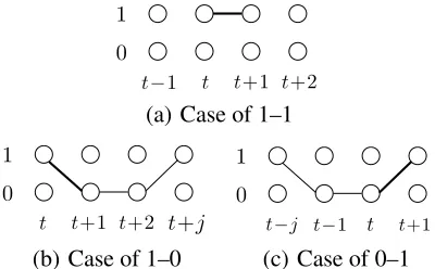
fea-tures associated with label bigrams in our binary CRF can be divided into four types: 1-1,1-0,0-1, and 0-0, as shown in Figure 7.
Case 1-1: As shown in Figure 8(a), this case means that a word of length 1 begins at timet, which is
equivalent to the probability of substringcttbeing
a word:
p(zt= 1, zt+1= 1|s) =p(ctt|s). (14)
Here,p(ckℓ|s)is the marginal probability of a
sub-stringcℓ· · ·ckbeing a word, which can be derived
from equation (12):
p(ckℓ|s) =X j
p(ckℓ, cℓℓ−j−1|s)
=X j
α[ℓ−1][j]·β[k][k−ℓ+1]·
exphλ0logp(ckℓ|cℓℓ−−1j) +γ[ℓ, k+1)
i
/Z(s)
= β[k][k−ℓ+1] Z(s) ·
X
j
expλ0logp(ckℓ|cℓℓ−−1j)
+γ[ℓ, k+1)α[ℓ−1][j]
= α[k][k−ℓ+1]·β[k][k−ℓ+1]
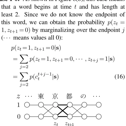
Z(s) (15) Case 1-0: As shown in Figure 8(b), this case means that a word begins at time t and has length at least 2. Since we do not know the endpoint of this word, we can obtain the probability p(zt= 1, zt+1= 0)by marginalizing over the endpointj
(· · · means values all 0):
p(zt= 1, zt+1= 0|s)
=X j=2
p(zt= 1, zt+1= 0,· · ·, zt+j= 1|s)
=X j=2
[image:5.612.322.542.466.687.2]p(ct+j−1t |s) (16)
(a) Case of 1–1
[image:6.612.83.283.58.182.2](b) Case of 1–0 (c) Case of 0–1
Figure 8: Label bigram potentials for marginalization. The probability of each label bigram (bold) of the Markov model can be obtained by marginalizing the probability of the U-shaped path including it, which is computed in the semi-Markov model.
wherep(ct+jt −1|s)is obtained from (15).
Case 0-1: Similarly, as shown in Figure 8(c) this case means that a word of length at least 2 begins before time t and ends at time t. Therefore, we
can marginalize over the start point of a possible word to obtain the marginal probability:
p(zt= 0, zt+1= 1|s)
=X j=1
p(zt−j= 1,· · ·, zt= 0, zt+1= 1|s) (17)
=X j=1
p(ctt−j|s). (18)
Case 0-0: In principle, this means that a word be-gins before timetand ends later than (and
includ-ing) time t+ 1. Therefore, we can marginalize over both the start and end time of a possible word spanning[t, t+1]to obtain:
p(zt= 0, zt+1= 0|s) =X j=1
X
k=1
p(ct+kt−j|s). (19)
However, in fact we can avoid this nested compu-tation because the probability ofp(zt, zt+1) over
the possible values of zt and zt+1 must sum to
1. We can therefore simply calculate it as follows (Andrew, 2006):
p(zt= 0, zt+1= 0|s) = 1−p(1,1)−p(1,0)−p(0,1)
(20) wherep(x, y)meansp(zt=x, zt+1=y|s). 4.3 Inference
Finally, we obtain the inference algorithm for NPY-CRF as a variant of the MCMC-EM algorithm (Wei
and Tanner, 1990) shown in Figure 9.2In learning of
a NPYLM, we add the CRF potentials as described in Section 4.1, and sample a possible segmenta-tion from the posterior through Forward filtering-Backward sampling to update the model parameters. On the basis of this improved language model, the CRF weights are then optimized by incorporating language model features as explained in Section 4.2. We iterate this process until convergence.
Note that we first have to learn an unsupervised segmentation in Step 2 before training the CRF. Since our inference algorithm includes an optimiza-tion of CRF and thus is not a true MCMC, the learn-ing of word segmentationafterthe supervised infor-mation will be severely constrained and likely to get stuck in local minima.
In practice, we found that the EM-style batch learning of CRF described above often fails because our objective function is non-convex. Therefore, we switched to ADF below (Sun et al., 2014), an adap-tive stochastic gradient descent that yields state-of-the-art accuracies for natural language processing problems including word segmentation. In this case,
Λ in Figure 9 was optimized with each minibatch
through the labeled datahXl, Yli, while
incorporat-ing information from the unlabeled dataXu by the
language model.
Because of its heavy computational demands,
1: AddhYl, Xlito NPYLM.
2: OptimizeΛonhYl, Xli. (pure CRF) 3: forj= 1· · ·Mdo
4: fori= randperm(1· · ·N)do 5: ifj >1then
6: Remove customers ofXu(i)from NPYLMΘ 7: end if
8: Draw segmentations ofXu(i)from NPYCRF 9: Add customers ofXu(i)to NPYLMΘ 10: end for
11: OptimizeΛof NPYCRF onhYl, Xli. 12: end for
Figure 9: Basic learning algorithm for NPYCRF. Xu(i) denotes thei-th sentence in the unlabeled dataXu. We can also iterate steps 4 to 10 several times untilΘ approx-imately converges, before updatingΛ.
Language Dataset Labeled Unlabeled Test
Chinese MSR 86,924 865,679 3,985 Weibo 10K-40K 880,920330,000
[image:7.612.69.308.53.127.2]Japanese Twitter 59,931 600,000 444 Thai InterBEST 10,000 30,133 10,000
Table 1: Statistics of the datasets for the experiments.
we parallelized the NPYLM sampling over sev-eral processors and because of the possible corre-lation of segmentations within the samples, used the Metropolis-Hastings algorithm to correct them. The acceptance rate in our experiments was over 99%.
For decoding, we can simply find a Viterbi path in the integrated semi-Markov model while fixing all the sampled segmentations on the unlabeled data.
5 Experiments
We conducted experiments on several corpora of un-segmented languages: Japanese, Chinese, and Thai. The corpora included standard corpora as well as text from Twitter and its equivalent, Weibo, in Chi-nese.
5.1 Data
Chinese For Chinese, we first used a standard dataset from the SIGHAN Bakeoff 2005 (Emerson, 2005) for the labeled and test data, and Chinese gi-gaword version 2 (LDC2009T14) for the unlabeled data. We chose the MSR subset of SIGHAN Bakeoff written in simplified Chinese together with the pro-vided training and test splits, which contain about 87K/40K sentences, respectively. For the unlabeled data, i.e., a collection of raw strings, we used a ran-dom subset of 880K sentences from Chinese giga-word with all spaces removed. We chose this size to be about 10 times larger than the labeled data, con-sidering current computational requirements. We used the part from the Xinhua news agency 2004 and split the data into sentences at the end-of-sentence character “。”.
Because the MSR and Xinhua datasets were com-piled from newspapers, to meet our objective on in-formal text we conducted further experiments using
3This is the total number of sentences in the experiment: the actual number of unsupervised sentences is this set minus the different number of supervised sentences.
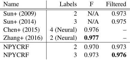
Name Labels F Filtered
Sun+ (2009) 2 N/A 0.973
Sun+ (2014) 3 N/A 0.975
Chen+ (2015) 4 (Neural) 0.976 – Zhang+ (2016) 2 (Neural) 0.977 –
NPYCRF 2 0.970 0.973
NPYCRF 3 0.973 0.976
Table 2: Accuracies of Bakeoff MSR dataset in Chinese. “Filtered” are the results with a simple post-hoc filter de-scribed in Sun et al. (2009).
Data Label Unlabel IV OOV F
Topline 880K – 0.981 0.699 0.977
Sup 10K 10K – 0.949 0.690 0.928 Sup 20K 20K – 0.957 0.683 0.941 Sup 40K 40K – 0.963 0.682 0.951 Semi 10K 10K 870K 0.954 0.698 0.933 Semi 20K 20K 860K 0.961 0.690 0.945 Semi 40K 40K 840K 0.970 0.648 0.955 Table 3: Accuracies on Leiden Weibo corpus in Chinese. ‘Label’ and ‘Unlabel’ are the amounts of labeled and un-labeled data, respectively. “Topline” is an ideal situation of complete supervision, and K= 103sentences.
the Leiden Weibo corpus4 from Weibo, a Twitter
equivalent in China. From this dataset, we used the sentences that have exact correspondence between the provided segmented-unsegmented pair, yielding about 880K sentences. Since we did not know how much supervision would be necessary for a decent performance, we conducted experiments with dif-ferent amounts of labeled data: 10K, 20K, 40K and 880K(all). Note that the final case amounts to com-plete supervision, an ideal situation that is not likely in practice.
Japanese Word segmentation accuracies around 99% have already been reported for newspaper do-mains in Japanese (Kudo et al., 2004). Therefore, we only conducted experiments on segmenting Twitter text. In addition to our random Twitter crawl in April 2014, we used a corpus of Japanese Twitter text compiled by the Tokyo Metropolitan University5.
This corpus is actually very small, 944 sentences. It mainly targets transfer learning and is segmented ac-cording to BCCWJ (Basic Corpus of Contemporary
[image:7.612.317.534.54.155.2]Written Japanese) standards from the National Insti-tute of Japanese Language (Maekawa, 2007). There-fore, for the labeled data we used the “core” subset of BCCWJ consisting of about 59K sentences plus 500 random sentences from the Twitter dataset. We used the remaining 444 sentences for testing. For the unlabeled data, we used a random crawl of 600K Japanese sentences collected from Twitter in March-April, 2014.
Thai Unsegmented languages, such as Thai, Lao, Myanmar, and Kumer, are also prevalent in South East Asia and are becoming increasingly important targets of natural language processing. Thus we also conducted an experiment on Thai, using the standard InterBEST 2009 dataset (Kosawat, 2009). Since it is reported that the “novel” subset of InterBEST has relatively low precision, we used this part with a ran-dom split of 10K sentences for supervised learning, 30K sentences for unsupervised learning, and a fur-ther 10K sentences for testing.
5.2 Training Settings
Because Sun et al. (2012) report increased accuracy with three tags, {B,I,E}6, we also tried these tags in place of the binary tags described in Section 4.2. This modification resulted in 6 possible transitions out of 32 = 9 transitions, whose computation
fol-lows from the binary case in Section 4.2. We used normal priors of truncated N(1, σ2) and N(0, σ2)
for λ0 and λ1· · ·λK, respectively, and fixed the
CRF regularization parameterCto1.0, andσto1.0
by preliminary experiments on the same data. For the feature templates, we followed Sun et al. (2012). In addition to those templates, we used char-acter type bigrams, where the ‘charchar-acter type’ was defined by Unicode blocks (like Hiragana or CJK Unified Ideographs for Chinese and Japanese) or Unicode character categories (Thai).
To reduce computations by restricting the search space appropriately, we employed a Negative Bi-nomial generalized linear model on string features (Uchiumi et al., 2015) to predict the maximum length of a possible word for each character position in the training data. Therefore, the upper limit ofL
in (11) and (13) wasLtfor each positiont, obtained 6The B, I, and E tags mean the beginning, internal part, and end of a word, respectively.
东软集团 19
游景玉 17
任尧森 17
南昆铁路 16 东方红三号”卫星 13
刘积仁 13
internet 11
东宝 11
张肇群 10
彭云 10
玲英 10
抚州 10
亚仿 10
南丁格尔 9
中远香港集团 7 海尔-波普彗星 7 第九届全国人民代表大会 6
巨型机 6
にゃん 6
セフレ 6
フォロワー 5 https 4 December 4 トナカイ 3 アオサギ 3 フォロバ 3
じゅん 3
環奈 3
リプ 3
トッキュウジャー 2 リフォロー 2 酔っ払い 2 ツイート 2 クシャミ 2 エタフォ 2 まじかよ 2
ググれ 2
ふりふり 2
[image:8.612.319.535.52.241.2](a) MSR (Simplified Chinese) (b) Twitter (Japanese)
Figure 10: New words acquired by NPYCRF. For each figure, the left column is the words that did not appear in the provided labeled data, and the right column is the frequencies NPYCRF recognized in the test data. In Chi-nese, we found many proper names including company and person name, and in Japanese, we found many novel slang words and proper names.
from this statistical model trained on labeled seg-mentations. We observed that this prediction made the computation several times faster than, for exam-ple, using a fixed threshold in Japanese where quite long words are occasionally encountered.
5.3 Experimental results
CRF NPYLM NPYCRF Gold
有些 有些 有些 有些
大学生 大学生 大学生 大学生
眼 眼高手低 眼 眼高手低
高手 高手
低 低
, , , ,
不屑 不屑于 不屑于 不屑于
于
做 做 做 做
小 小 小 小
事情 事情 事情 事情
。 。 。 。
王思斌 王 王思斌 王思斌
思 斌
, , , ,
男 男 男 男
, , , ,
1949年10月 1949年 1949年10月 1949年10月 10月
生 生 生 生
。 。 。 。
Figure 11: Example of segmentation of the SIGHAN Bakeoff MSR dataset made with supervised (CRF), un-supervised (NPYLM), and semi-un-supervised (NPYCRF) models in comparison with gold segmentations (Gold). “眼高手低” is a proverb and “王思斌” is a full name of a person.
available in practice. In fact, we realized that the Weibo segmentations were given automatically by an existing classifier, and contain many inappropri-ate segmentations, while NPYCRF finds much “bet-ter” segmentations.
Figure 11 compares the results of CRF, NPYLM, and NPYCRF with the gold segmentation. While proverbs like “眼高手低” (wide vision without ac-tion) are correctly captured from the unlabeled data by NPYLM, it is sometimes broken by CRF through integration. In another case, the name of a per-son is properly connected because of the informa-tion provided by the CRF. This comparison shows that there is still room for improvement in NPYCRF. Section 6 discusses future research directions for im-provements.
Japanese and Thai Figure 12 shows an example of the analysis of Japanese Twitter text. Shaded words are those that are not contained in labeled data (BCCWJ core) but were found by NPYCRF. Many segmentations, including new words, are cor-rect. We expect NPYCRF would perform better with more unlabeled data that are easily obtained.
Tables 4 and 5 show the segmentation accuracies of the Twitter data in Japanese and novel data in
いや 他 で も 普通 に する よ シシルス サーチ 用 に ボーナス 持ちピン と か も ある し
誰 だ スズカ エルフォトン に ぶっこん だ の… 電車 で 座っ て ん だ けど 、 目 の 前 が 酔っ払い が 吊革 で フラフラ し て て ハラハラ する … 手遅れ に な ら ない うち に 離脱 する か …
ひこ にゃん 音頭 だ にゃん ♪ ひこ にゃん ひこ にゃん ひこ にゃん にゃん っ
ほんと です よ ほんと 嬉しい くっそ 倍率 やば そう 、 、 、 ほんと それ ! ! みほりん と 参戦 し たい まぢ で みほりんまま に も 会い たい
初めまして ♪ 私 は 絢瀬 絵里 役 の 鈴々 蝶 です ♪ 似 て ない です が 、 応援 し て くれる と 嬉しい です ♪ ちょくちょく 絡みだす なら なw w wこれ から も ちょ くちょく 絡む から よろしく (`ω´)
Figure 12: Samples of NPYCRF segmentation of Twit-ter text in Japanese that are difficult to analyze by ordi-nary supervised segmentation. It contains a lot of novel words, emoticons, and colloquial expressions that are not contained in the BCCWJ core text (shaded).
Thai. While there are no publicly available results for these data (the InterBEST testset is closed dur-ing competition), NPYCRF achieved better accura-cies than vanilla supervised segmentation based on CRF. Considering that many new words were found in Figure 12, for example, we believe NPYCRF is quite competitive thanks to its ability to learn the in-finite vocabulary, which it inherits from NPYLM.
6 Analysis
As shown in Figure 11, NPYCRF makes good use of NPYLM but sometimes ignores its prediction by falling back to CRF, yielding suboptimal perfor-mance. This is mainly because the geometric in-terpolation weight λ0 is always constant and does
not vary according to the input. For example, even if the substring to segment is very rare in the la-beled data, NPYCRF trusts the supervised classi-fier (CRF) with a constant rate of1/(1+λ0)in the
log probability domain. To alleviate this problem,
Model IV OOV F
CRF 0.939 0.706 0.916 NPYCRF 0.947 0.708 0.921 Table 4: Accuracies for Twitter text in Japanese.
Model IV OOV F
CRF 0.961 0.409 0.948 NPYCRF 0.959 0.362 0.954
it is necessary to change λ0 depending on the
in-put string in a log-linear framework.7 While this
might be achieved through Density Ratio estimation framework (Sugiyama et al., 2012; Tsuboi et al., 2009), we believe it is a general problem of semi-supervised learning and is beyond the scope of this paper.
This issue also affects the estimation of λ0 as a
scalar: that is, we found thatλ0often fluctuates
dur-ing traindur-ing because Λ (which includes λ0) is
esti-mated using only limitedhXl, Yli. In practice, we
terminated the EM algorithm in Figure 9 early af-ter a few iaf-terations. Therefore, with a more adaptive semi-supervised learning framework, we expect that NPYCRF will achieve higher accuracy than the cur-rent performance.
7 Conclusion
In this paper, we presented a hybrid genera-tive/discriminative model of word segmentation, leveraging a nonparametric Bayesian model for un-supervised segmentation. By combining CRF and NPYLM within the semi-supervised framework of JESS-CM, our NPYCRF not only works as well as the state-of-the-art neural segmentation without hand tuning of hyperparameters on standard cor-pora, but also appropriately segments non-standard texts found in Twitter and Weibo, for example, by automatically finding “new words” thanks to a non-parametric model of infinite vocabulary.
We believe that our model lays the foundation for developing a methodology of combining nonpara-metric Bayesian models and discriminative classi-fiers, as well as providing an example of semi-supervised learning on different model structures, i.e. Markov and semi-Markov models for word seg-mentation.
Acknowledgments
We are deeply grateful to Jun Suzuki (NTT CS Labs) for important discussions leading to this re-search, Xu Sun (Peking University) for details of his experiments in Chinese. We would also like to thank anonymous reviewers and the action editor,
7This is reminiscent of context-dependent Bayesian smooth-ing of MacKay (1994) in the probability domain, as opposed to the fixed Jelinek-Mercer smoothing (Goodman, 2001).
especially the editors-in-chief for the thorough com-ments for the final manuscript.
References
Galen Andrew. 2006. A Hybrid Markov/Semi-Markov Conditional Random Field for Sequence Segmenta-tion. InEMNLP 2006, pages 465–472.
Xinchi Chen, Xipeng Qiu, Chenxi Zhu, and Xuanjing Huang. 2015. Gated Recursive Neural Network for Chinese Word Segmentation. In ACL 2015, pages 1744–1753.
Gregory Druck and Andrew McCallum. 2010. High-Performance Semi-Supervised Learning using Dis-criminatively Constrained Generative Models. In ICML 2010, pages 319–326.
Tom Emerson. 2005. The Second International Chinese Word Segmentation Bakeoff. In Proceedings of the Fourth SIGHAN Workshop on Chinese Language Pro-cessing.
Sharon Goldwater, Thomas L. Griffiths, and Mark John-son. 2006. Contextual Dependencies in Unsupervised Word Segmentation. InProceedings of ACL/COLING 2006, pages 673–680.
Joshua T. Goodman. 2001. A Bit of Progress in Lan-guage Modeling, Extended Version. Technical Report MSR–TR–2001–72, Microsoft Research.
Jahn Heymann, Oliver Walter, Reinhold H¨ab-Umbach, and Bhiksha Raj. 2014. Iterative Bayesian Word Segmentation for Unsupervised Vocabulary Discov-ery from Phoneme Lattices. In ICASSP 2014, pages 4057–4061.
Krit Kosawat. 2009. InterBEST 2009: Thai Word Seg-mentation Workshop. InProceedings of 2009 Eighth International Symposium on Natural Language Pro-cessing (SNLP2009), Thailand.
Canasai Kruengkrai, Kiyotaka Uchimoto, Junichi Kazama, Kentaro Torisawa, Hiroshi Isahara, and Chuleerat Jaruskulchai. 2009. A word and character-cluster hybrid model for Thai word segmentation. In Eighth International Symposium on Natural Lanugage Processing.
Taku Kudo, Kaoru Yamamoto, and Yuji Matsumoto. 2004. Applying Conditional Random Fields to Japanese Morphological Analysis. InEMNLP 2004, pages 230–237.
John Lafferty, Andrew McCallum, and Fernando Pereira. 2001. Conditional Random Fields: Probabilistic Mod-els for Segmenting and Labeling Sequence Data. In Proc. of ICML 2001, pages 282–289.
David J. C. MacKay and L. Peto. 1994. A Hierarchical Dirichlet Language Model. Natural Language Engi-neering, 1(3):1–19.
Kikuo Maekawa. 2007. Kotonoha and BCCWJ: Devel-opment of a Balanced Corpus of Contemporary Writ-ten Japanese. In Corpora and Language Research: Proceedings of the First International Conference on Korean Language, Literature, and Culture, pages 158– 177.
Daichi Mochihashi and Eiichiro Sumita. 2008. The Infi-nite Markov Model. InAdvances in Neural Informa-tion Processing Systems 20 (NIPS 2007), pages 1017– 1024.
Daichi Mochihashi, Takeshi Yamada, and Naonori Ueda. 2009. Bayesian Unsupervised Word Segmentation with Nested Pitman-Yor Language Modeling. In Pro-ceedings of ACL-IJCNLP 2009, pages 100–108. Tomoaki Nakamura, Takayuki Nagai, Kotaro Funakoshi,
Shogo Nagasaka, Tadahiro Taniguchi, and Naoto Iwa-hashi. 2014. Mutual Learning of an Object Concept and Language Model Based on MLDA and NPYLM. In2014 IEEE/RSJ International Conference on Intel-ligent Robots and Systems (IROS’14), pages 600–607. ThuyLinh Nguyen, Stephan Vogel, and Noah A. Smith. 2010. Nonparametric Word Segmentation for Ma-chine Translation. InCOLING 2010, pages 815–823. Sunita Sarawagi and William W. Cohen. 2005.
Semi-Markov Conditional Random Fields for Information Extraction. InAdvances in Neural Information Pro-cessing Systems 17 (NIPS 2004), pages 1185–1192. Steven L. Scott. 2002. Bayesian Methods for Hidden
Markov Models. Journal of the American Statistical Association, 97:337–351.
Masashi Sugiyama, Taiji Suzuki, and Takafumi Kanamori. 2012. Density Ratio Estimation in Machine Learning. Cambridge University Press. Weiwei Sun and Jia Xu. 2011. Enhancing Chinese Word
Segmentation using Unlabeled Data. InEMNLP 2011, pages 970–979.
Xu Sun, Yaozhong Zhang, Takuya Matsuzaki, Yoshimasa Tsuruoka, and Jun’ichi Tsujii. 2009. A Discrimina-tive Latent Variable Chinese Segmenter with Hybrid Word/Character Information. InNAACL 2009, pages 56–64.
Xu Sun, Houfeng Wang, and Wenjie Li. 2012. Fast On-line Training with Frequency-Adaptive Learning Rates for Chinese Word Segmentation and New Word Detec-tion. InACL 2012, pages 253–262.
Xu Sun, Wenjie Li, Houfeng Wang, and Qin Lu. 2014. Feature-Frequency-Adaptive Online Training for Fast and Accurate Natural Language Processing. Compu-tational Linguistics, 40(3):563–586.
Jun Suzuki and Hideki Isozaki. 2008. Semi-Supervised Sequential Labeling and Segmentation Using Giga-Word Scale Unlabeled Data. InACL:HLT 2008, pages 665–673.
Yee Whye Teh. 2006. A Hierarchical Bayesian Lan-guage Model based on Pitman-Yor Processes. In Pro-ceedings of ACL/COLING 2006, pages 985–992. Yuta Tsuboi, Hisashi Kashima, Shohei Hido, Steffen
Bickel, and Masashi Sugiyama. 2009. Direct Den-sity Ratio Estimation for Large-scale Covariate Shift Adaptation. Information and Media Technologies, 4(2):529–546.
Kei Uchiumi, Hiroshi Tsukahara, and Daichi Mochi-hashi. 2015. Inducing Word and Part-of-speech with Pitman-Yor Hidden Semi-Markov Models. In ACL-IJCNLP 2015, pages 1774–1782.
Greg C.G. Wei and Martin A. Tanner. 1990. A Monte Carlo Implementation of the EM Algorithm and the Poor Man’s Data Augmentation Algorithms. Journal of the American Statistical Association, 85(411):699– 704.