Breaking the Closed World Assumption in Text Classification
Geli Fei
and
Bing Liu
Department of Computer Science
University of Illinois at Chicago
[email protected], [email protected]
Abstract
Existing research on multiclass text classific
a-tion mostly makes the closed world assump-tion, which focuses on designing accurate classifiers under the assumption that all test classes are known at training time. A more re-alistic scenario is to expect unseen classes during testing (open world). In this case, the goal is to design a learning system that classi-fies documents of the known classes into their respective classes and also to reject docu-ments from unknown classes. This problem is called open (world) classification. This paper
approaches the problem by reducing theopen space risk while balancing the empirical risk. It proposes to use a new learning strategy, called center-based similarity (CBS) space learning (or CBS learning), to provide a novel solution to the problem. Extensive e xperi-ments across two datasets show that CBS learning gives promising results on multiclass open text classification compared to state-of-the-art baselines.
1
Introduction
With the rapid growth of online information, text classifiers have become one of the most important tools for people to track and organize information. And the emergence of social media platforms has brought increasing diversity and dynamics to the Web. Many social science researchers rely on the collected online user generated content to carry out research on different social phenomenon. In this case, multiclass text classifiers are widely used to gather information of several topics of interest. However, most existing research on multiclass text classification makes the closed world assumption, meaning that all the test classes have been seen in training. However, in a more realistic scenario
where people use a multiclass classifier to collect information of several topics from a data source that covers a much broader range of topics, it is normal to break the closed world assumption and to see the arrival of documents from unknown classes that have never been seen in training. In this case, a multiclass classifier should not always assign a document to one of the known classes. In-stead, it should identify unknown classes of docu-ments and label them as unknown or reject. This is called open (world) classification.
More precisely, in the traditional multiclass classification setting, the learner assumes a fixed set of classes Y = {C1, C2, …, Cm}, and the task is to construct a 𝑚-class classifier using the training data. The resulting classifier is tested/applied on the data from only the m classes. While in open classification, we allow the classifier to predict la-bels/classes from the set of C1, C2, …, Cm, Cm+1 classes, where the (m+1)th class C
m+1 represents the unknown which covers documents of all unknown or unseen classes or topics. In other words, every test instance may be predicted to belong to either one of the known classes yi∈𝑌, or Cm+1 (un-known).
It is thus not sufficient for a classifier to just re-turn the most likely class label among the m known classes. An option to reject must be provided. An obvious approach to predicting the class label
𝑦∈𝑌∪{𝐶!!!} for an n-dimensional data point 𝑥∈𝑅! is to incorporate a posterior probability es-timator 𝑝(𝑦|𝑥) and a decision threshold into an ex-isting multiclass learning algorithm (Kwok, 1999; Fumera and Roli, 2002; Huang et al., 2006; Bravo et al., 2008). There are many reasons this tech-nique would not achieve good results in open clas-sification. As we will discuss in the following sec-tions, one of the most important reasons is that the underlying classifier is not robust or is not
formed enough to reject unseen classes of docu-ments due to its significant open space risk.
Traditional multiclass learners optimize only on the known classes under the closed world assump-tion, while a potential learner for open classifica-tion has to optimize for both the known classes and for the unknown classes. Some recent research in the field of computer vision studied the problem, which they call open set recognition (Scheirer et al., 2013; 2014; Jain et al., 2014) for facial recog-nition. Classic learners define and optimize over empirical risk, which is measured on the training data. For open classification, it is crucial to consid-er how to extend the model to capture the risk of the unknown by preventing overgeneralization or overspecialization. In order to tackle this problem, Scheirer et al. (2013) introduced the concept of open space risk and formulated an extension of ex-isting one-class and binary SVMs to address the open classification problem. However, as we will see in section 3, their proposed method is weak as the positively labeled open space is still an infinite area.
In this work, we propose a solution to reduce the open space risk while also balancing the empirical risk for open classification. Intuitively, given a positive class of documents, our open space for the positive class is considered as the space that is suf-ficiently far from the center of the positive docu-ments. In the multiclass classification setting, each of the m target classes is surrounded by a ball cov-ering the positively labeled (the target class) area, while any document falling outside of all the m balls is considered belonging to the unknown class.
Recent work by Fei and Liu (2015) proposed a new learning strategy called center-based similari-ty space learning (CBS learning) to deal with the problem of covariate shift in binary classification. We found that it is also suitable for open classifica-tion. Instead of conducting learning in the tradi-tional document space (or D-space) with n-gram features, CBS learning learns in a similarity space. Unlike SVM learning in D-space that bounds the positive class only by an infinite half-space formed with the decision hyperplane, which has a huge open space risk, CBS learning finds a closed boundary for the positive class covering only a fi-nite area, which is a spherical area in the original D-space and thus reduce the open space risk signif-icantly. While discussing CBS learning, we will al-so describe the underlying assumptions made by it
which were not stated in our earlier paper (Fei and Liu, 2015). Our final multiclass classifier is called cbsSVM (based on SVM).
To the best of our knowledge, this is the first at-tempt to study multiclass open classification in text from the open space risk management perspective. Our experiments show that cbsSVM for multiclass open classification produces superior classifiers to existing state-of-the art methods.
2
Related Work
Compared to research on multiclass classification with the closed world assumption, there is relative-ly less work on open classification. In this section, we review related work on one-class classification, SVM decision score calibration, and others.
One-class classifiers, which only rely on posi-tive training data, are natural starting solutions to the multiclass open classification task. One-class SVM (Scholkopf et al., 2001) and SVDD (Tax and Duin, 2004) are two representative one-class clas-sifiers. One-class SVM treats the origin in the fea-ture space as the only member of the negative class, and maximizes the margin with respect to it. SVDD tries to place a hypersphere with the mini-mum radius around almost all the positive training points. It has been shown that the use of Gaussian kernel makes SVDD and One-class SVM equiva-lent, and the results reported in (Khan and Madden, 2014) demonstrate that SVDD and One-class SVM are comparable when the Gaussian kernel is ap-plied. However, as no negative training data is used, one-class classifiers have trouble producing good separations. We will see in Section 4 that their results are poor.
probabil-ity of this instance belonging to a class is lower than the threshold in multiclass open classification settings.
Recently, researchers in computer vision (Scheirer et al., 2013; 2014; Jain et al., 2014) made some attempts to solve open classification (which they call open set recognition) for visual learning from new angles. Scheirer et al. (2013) introduced the concept of open space risk, and defined it as a relative measure. The proposed model reduces the open space risk by replacing the half-space of a bi-nary linear classifier with a positive region bound-ed by two parallel hyperplanes. While the positive-ly labeled region for a target class is reduced com-pared to the half-space in the traditional linear SVM, their open space risk is still infinite. In (Jain et al., 2014), the authors proposed to use Extreme Value Theory (EVT) to estimate the unnormalized posterior probability of inclusion for each class by fitting a Weibull distribution over the positive class scores from a 1-vs-rest multiclass RBF SVM clas-sifier. Scheirer et al. (2014) introduced the Com-pact Abating Probability (CAP) model, which ex-plains how thresholding the probabilistic output of RBF One-class SVM manages the open space risk. Using the probability output from RBF one-class SVM as a conditioner, the authors combine RBF One-class SVM and a Weibull-calibrated SVM similar to the one in (Jain et al., 2014). For both methods (Jain et al., 2014; Scheirer et al., 2014), decision thresholds need to be chosen based on the prior knowledge of the ratio of unseen classes in testing, which is a weakness of the methods.
Dalvi et al. (2013) proposed Exploratory Learn-ing in the multiclass semi-supervised learnLearn-ing (SSL) setting. In their work, an “exploratory” ver-sion of expectation-maximization (EM) is pro-posed to extend traditional multiclass SSL meth-ods, which deals with the scenario when the algo-rithm is given seeds from only some of the classes in the data. It automatically explores different numbers of new classes in the EM iterations. The underlying assumption is that a new class should be introduced to hold an instance 𝑥 when the prob-ability of 𝑥 belonging to the existing classes is close to uniform. This is quite different from our work. First, it works in the semi-supervised setting and assumes that test data is available during train-ing. Second, it only focuses on improving accuracy on the classes with seed examples.
3
Proposed Method
In this section, we propose our solution for the open classification problem. First we discuss our strategy to reduce the open space risk while bal-ancing the empirical risk of the training data. Then we apply a recently proposed SVM-based learning strategy (Fei and Liu, 2015), which yields the same risk management strategy. We will also discuss its underlying assumptions, which was not addressed in the original paper of Fei and Liu (2015). Lastly, we will show why the proposed solution works for open classification.
3.1
Open Space Risk FormulationConsider the risk formulation by Scheirer et al. (2013), where apart from the empirical risk, there is risk in labeling the open space (space away from positive training examples) as “positive” for any known class. Due to lack of information on a clas-sification function on the open space, open space risk is approximated by a relative Lebesgue meas-ure (Shackel, 2007). Let 𝑆! be a large ball of radius 𝑟! that contains both the positively labeled open space 𝑂 and all of the positive training examples; and let 𝑓 be a measurable classification function where 𝑓! 𝑥 =1 for recognition of class 𝑦 of in-terest and 𝑓! 𝑥 =0 otherwise. The probabilistic open space risk 𝑅! 𝑓 of function 𝑓 for a class 𝑦 is defined as the fraction (in terms of Lebesgue measure) of positively labeled open space com-pared to the overall measure of positively labeled space (which includes the space close to the posi-tive examples).
𝑅! 𝑓 =
𝑓! 𝑥 𝑑𝑥 !
𝑓! 𝑥 𝑑𝑥 !!
The above definition indicates that the more we label open space as positive, the greater open space risk is. However, it does not suggest how to speci-fy the positively labeled open space 𝑂.
center 𝑐𝑒𝑛!. Let classification function 𝑓! 𝑥 =1 when 𝑥∈𝐵!! 𝑐𝑒𝑛! , and 𝑓! 𝑥 =0 otherwise. Also let ℎ be the positive half space defined by a binary SVM decision hyperplane Ω obtained using positive and negative training examples, and let the size of ball 𝐵!! be bounded by Ω, 𝐵!!⋂ℎ=𝐵!!. We define open space as
𝑂=𝑆!−𝐵!! 𝑐𝑒𝑛!
where radius 𝑟! needs to be determined from the training data for each known positive class.
This open space formulation greatly reduces the open space risk compared to traditional SVM and 1-vs-Set Machine in (Scheirer et al., 2013). For traditional SVM, whose classification function 𝑓!!"# 𝑥 =1 when 𝑥∈ℎ, and positive open space being approximately ℎ−𝐵!! 𝑐𝑒𝑛! , which is only bounded by the SVM decision hyperplane Ω. For 1-vs-Set Machine in (Scheirer et al., 2013), whose classification function 𝑓!!!!"!!"# 𝑥 =1 when
𝑥∈𝑔, where 𝑔 is a slab area with thickness 𝛿
bounded by two parallel hyperplanes Ω and Ψ (Ψ∥Ω) in ℎ. And its positive open space is ap-proximately 𝑔−𝐵!! 𝑐𝑒𝑛! . Given open space formulations of traditional SVM and 1-vs-Set Ma-chine, we can see that both methods label an un-limited area as positively labeled space, while our formulation reduces it to a bounded spherical area.
Given the above open space definition, the ques-tion is how to estimate radius 𝑟! for the positive
class. We show that the center-based similarity space learning (CBS learning) recently proposed in (Fei and Liu, 2015) is suitable for the purpose. It was original proposed to deal with the negative co-variate shift problem in binary text classification.
Below, we first introduce CBS learning and then discuss why it is suitable for our problem, as well as its underlying assumptions.
3.2
Center-Based Similarity Space Learning We now discuss CBS learning for binary text clas-sification. Let D = {(d1, y1), (d2, y2), …, (dn, yn)} be the set of training examples, where di is the fea-ture vector (e.g., with unigram feafea-tures) represent-ing a document di and yi∈ {1, -1} is its class label.This feature vector is called a document space vec-tor (ds-vector). Traditional classification directly uses D to build a binary classifier. CBS learning
transforms each ds-vector di (no change to its class) to a center-based similarity space feature vector (CBS vector) cbs-vi. Each feature in the CBS vec-tor is a similarity between a center cj of the positive class documents and di. CBS learning can use mul-tiple document space representations or feature vectors (e.g., one based on unigrams and one based on bigrams) to represent each document, which re-sults in multiple centers for the positive documents. There can also be multiple document similarity functions used to compute similarity values. The detailed learning technique is as follows.
For a document di in D, we have a set Ri of pds -vectors Ri = {𝐱!!, 𝐱!!, …, 𝐱!!}. Each ds-vector 𝐱!! denotes one document space representation of the document di, e.g., unigram representation or bi-gram representation. Then the center of positive training documents can be computed, which is rep-resented as a set of 𝑝 centroids C= {c1, c2, …, cp}, each of which corresponds to one document space representation in Ri. Rocchio method in infor-mation retrieval (Rocchio, 1971; Manning et al. 2008) is used to compute each center cj (a vector), which uses the corresponding ds-vectors of all training positive and negative documents.
𝐜!= 𝛼 𝐷!
𝐱!! 𝐱!! −
𝛽
|𝐷−𝐷!|
𝐱!! 𝐱!! !!∈!!!!
!!∈!!
where 𝐷! is the set of documents in the positive class and |.| is the size function. 𝛼and 𝛽are pa-rameters, which are usually set empirically. It is reported that using tf-idf representation, 𝛼=16 and 𝛽=4 usually work quite well (Buckley et al. 1994). The subtraction is used to reduce the influ-ence of those terms that are not discriminative (i.e., terms appearing in both classes).
Based on Ri for any document di in both training and testing and the previously computed set C of centers using the training data, we can transform a document di from its document space representa-tions Ri to one center-based similarity vector cbs-vi by applying a similarity function 𝑆𝑖𝑚 on each ele-ment 𝐱!! of Ri and its corresponding center 𝐜! in C.
cbs-vi = Sim(Ri, C)
For ds-features, we use unigrams and bigrams with tf-idf weighting as two document representa-tions. We also adopt the five similarity measures in (Fei and Liu, 2015) to gauge the similarity of two vectors. Based on these measures, we produce 10 CBS features to represent a document in the CBS space.
3.3
Why does CBS learning work?Given the open space definition in Section 3.1, our goal is to estimate the radius 𝑟! of the positively labeled space for the positive class. Now we ex-plain how CBS learning gives an estimate of 𝑟!.
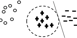
Due to learning in the similarity space with similarities as features, CBS learning generates a boundary based on similarities to separate the posi-tive and negaposi-tive training data in the similarity space, which is essentially a ball encompassing the positive training data in the original document space. In other words, instead of explicitly mini-mizing the positively labeled open space risk, CBS learning approximates the radius 𝑟! by learning a score based on similarities in the similarity space, which is equivalent to a limited spherical area in the original document space. The generated model thus not only limits the positively labeled open space on the positive side of Ω (SVM decision hy-perplane), but also balances the empirical risk from the positive and negative training examples. In fact, 𝑟! is approximately the distance from the cen-ter of positive class to Ω measured in similarities. Figure 1 illustrates the point. The positively la-beled/classified region produced by CBS learning is the circle in the original document space, while SVM learning produces a half space bounded by its decision line, which is approximately the tan-gent line of the circle. Note that as multiple simi-larity features are used, the spherical area is formed by an integrated similarity produced by SVM, which combines all similarity features.
In order for the method to work well for our multiclass classification, ideally two assumptions should be made about the data. First, the target
classes of documents are generated by a mixture model, where each mixture component is respon-sible for each class of documents. Secondly, after feature normalization each target class of docu-ments is generated by a Gaussian distribution, where the Gaussian mean resides at the center of the class, and its 𝑛×𝑛 covariance matrix has equal eigenvalues so that the positive class can have a spherical shape boundary or a ball. Note that we do not make any assumptions about data from non-target classes.
3.4
Multiclass Open ClassificationThe preceding discussion is based on binary open classification. We follow the standard technique of combining a set of 1-vs-rest binary classifiers to perform multiclass classification with a rejection option for unknown. The SVM scores for each classifier are first converted to probabilities based on a variation of Platt’s (2000) algorithm, which is supported in LIBSVM (Chang and Lin, 2011). Let 𝑃 𝑦|𝐱 be a probably estimate, where 𝑦 ∈𝑌 is a class label and 𝐱 is a feature vector, and let 𝜆 be the decision threshold (usually 0.5). Let 𝑌 be the set of known classes, 𝐶!!! be the unknown class, and 𝑦∗ is the final predicted class for x. The final
classifier (called cbsSVM) uses this following for classification.
𝑦∗= 𝑎𝑟𝑔𝑚𝑎𝑥!∈𝑌𝑃
𝑦|𝐱
𝑖𝑓𝑃𝑦
∗|𝐱 ≥𝜆𝐶𝑚+1 𝑜𝑡ℎ𝑒𝑟𝑤𝑖𝑠𝑒
4
Experiments
In this section, we show the results of the proposed method cbsSVM and compare it extensively with state-of-the-art baselines across two datasets.
4.1
Baselines1-vs-Rest multiclass SVM (1-vs-rest-SVM). This is the standard 1-vs-Rest multiclass SVM with Platt Probability Estimation (Platt, 2000), and it is implemented based on LIBSVM1 (version 3.20) (Chang and Lin, 2011). It works in the same way as the proposed cbsSVM (Section 3.4) except that it uses the document space classification. Linear ker-nel is used as it is shown by many researchers that linear SVM performs the best for text classification
[image:5.612.108.235.65.129.2]1 http://www.csie.ntu.edu.tw/~cjlin/libsvmtools/
(Joachims, 1998; Colas and Brazdil, 2006). 1-vs-Set Machine (1-vs-set-linear). For this base-line (Scheirer et al., 2013), we use all the default parameter settings in the original paper. That is, the near and far plane pressures are set at 𝑝! =1.6 and 𝑝! =4 respectively; regularization constant 𝜆! =1 and no explicit hard constraints are used on the training error (𝛼=0,𝛽=1).
W-SVM (wsvm-linear and wsvm-rbf). These two baselines combine RBF one-class SVM with bina-ry SVM (Scheirer et al., 2014). Both linear kernel and RBF kernel are tested. For thresholding the output, two parameters 𝛿! and 𝛿! are required. We set 𝛿!=0.001, which is used to adjust what data the one-class SVM considers to be related. 𝛿! is a
required decision threshold not only for W-SVM, but also for the next two baselines (PI-SVM, PI -OSVM). Two ways of setting 𝛿! were suggested by the authors. We set it as the prior probability of the number of unseen classes during evaluation (testing). An alternative way is to set it based on an openness score computed using the number of training and testing classes. We tried both methods and found the former gave better results.
PI-SVM (Pi-svm-linear and Pi-svm-rbf). This
baseline is from (Jain et al., 2014), which estimates the probability of inclusion based on the output of binary SVMs. Two kernels are tested. As stated above, the threshold 𝛿 is set as the prior probability of the number of unseen classes in test.
PI-OSVM (Pi-osvm-linear and Pi-osvm-rbf).
Sim-ilar to PI-SVM, PI-OSVM (Jain et al., 2014) uses a multiclass one-class SVM before fitting an Ex-treme Value Theory distribution to estimate the probability of inclusion. Again, two kernel func-tions are tested and the prior probability of the number of unseen classes is used to set 𝛿. As PI -OSVM is a variant of the traditional one-class SVM, we do not use one-class SVM as a baseline. Exploratory Seeded K-Means (Exploratory-EM). In (Dalvi et al., 2013), three well-known multiclass semi-supervised learning methods were extended under the exploratory EM framework. We compare with exploratory version of Seeded K-Means due to its superior performance on 20newsgroup dataset. We also applied the criteria that work the best in the original paper for creating new classes and for model selection, i.e., the
MinMax criterion and the AICc criterion. Note that ExploratoryEM works in the semi-supervised set-ting and uses both the training and test data as la-beled and unlala-beled data in training. As more than one new class can be introduced during training, for comparison we lump together all instances as-signed to new classes as being rejected (unknown). In the experiments, we set the max number of it-erations to be 50. Little changes in results are shown after 50 iterations.
All documents use tf-idf term weighting scheme with no feature selection. Source code for different baselines (1-vs-Set Machine2, W-SVM and P
I -SVM3, and Exploratory learning4) was provided by the authors of their original papers.
4.2
DatasetsWe perform evaluation using two publically avail-able datasets: 20-newsgroup (Rennie, 2008) and Amazon reviews (Jindal and Liu, 2008). The 20-newsgroup data contains 20 non-overlapping clas-ses with a total of 18828 documents. The Amazon reviews dataset has review documents of 50 types of products or domains. Each type of product has 1000 reviews. For each class in both datasets, we randomly sampled 70% of documents for training, and the rest 30% for testing. Although product re-views are used for experiments, we do not perform sentiment classification. Instead, we still perform the traditional topic based classification. That is, given a review, the system decides what type of product the review is about.
4.3
Experiment settingsFollowing that in (Jain et al., 2013) and (Dalvi et al., 2013), we conduct open world cross-validation style analysis, holding out some classes in training and mixing them back during testing, and varying the number of training and test classes. Since for a given dataset, the number (percentage) of training classes 𝑚 and the number of test classes 𝑛 can vary, there are many ways to generate a train-test partition. We report our results using 10 random train-test partitions for each dataset. We vary the number of test classes for Amazon (10, 20, 30, 40, 50), and for 20-newsgroup (10, 20). We use 25%,
2 https://github.com/Vastlab/liblinear.git 3 https://github.com/ljain2/libsvm-openset
50%, 75% and 100% of the test classes in training. When 100% of test classes are used in training, the problem reduces to the closed world classifica-tion. As most of our baselines such as W-SVM, PI -OSVM and PI-SVM all use prior knowledge to set decision threshold to 0 in the closed world setting, for fair comparison, we also set the threshold to 0 for both 1-vs-rest-SVM and our proposed cbsSVM for closed world classification. By doing this, we always assign a known class label to a test in-stance. For Exploratory Seeded K-Means, we use an option supported in the exploratory learning package that does not allow any new classes to be introduced in learning.
For each train-test partition, we first compute precision, recall and F1 score for each class and then macro-average the results across all classes.
Final results are given by averaging the results of 10 random train-test partitions. Due to space limits, we will only show F1 scores in the paper.
For all the methods that use the RBF kernel, the parameters are tuned via cross validation on the training data, yielding (𝐶=5,𝛾=0.2) for Ama-zon and (𝐶 =10,𝛾=0.5) for 20-newsgroup.
4.4
Results and DiscussionWe now show all the results. Results for Amazon is given in Tables 1 to 5, and for 20-newsgroup are given in Tables 6 and 7. As we can see, in most situations (23 of 28 settings) our proposed cbsSVM method performs the best. Even when 100% of the test classes are used for training (the traditional closed world classification), cbsSVM still performs
25% 50% 75% 100% 25% 50% 75% 100% 25% 50% 75% 100% cbsSVM 0.450 0.715 0.775 0.873 0.566 0.695 0.695 0.760 0.565 0.645 0.630 0.686 1-vs-rest-SVM 0.219 0.658 0.715 0.817 0.466 0.610 0.616 0.688 0.463 0.568 0.545 0.627 ExploratoryEM 0.386 0.647 0.704 0.854 0.571 0.561 0.573 0.691 0.500 0.511 0.569 0.659 1-vs-set-linear 0.592 0.698 0.700 0.697 0.506 0.560 0.589 0.620 0.462 0.511 0.542 0.585 wsvm-linear 0.603 0.694 0.698 0.702 0.553 0.618 0.625 0.641 0.521 0.574 0.578 0.598 wsvm-rbf 0.246 0.587 0.701 0.792 0.397 0.502 0.574 0.701 0.372 0.444 0.502 0.651 Pi-osvm-linear 0.207 0.590 0.662 0.731 0.453 0.531 0.589 0.629 0.428 0.510 0.553 0.605 Pi-osvm-rbf 0.061 0.142 0.137 0.148 0.143 0.079 0.058 0.050 0.108 0.047 0.043 0.047 Pi-svm-linear 0.600 0.695 0.701 0.705 0.547 0.620 0.628 0.644 0.520 0.575 0.581 0.602 Pi-svm-rbf 0.245 0.590 0.718 0.774 0.396 0.546 0.675 0.714 0.379 0.517 0.629 0.680 Table 1: Amazon 10 Domains. Table 2: Amazon 20 Domains. Table 3: Amazon 30 Domains.
25% 50% 75% 100% 25% 50% 75% 100% cbsSVM 0.541 0.633 0.619 0.650 0.557 0.615 0.586 0.634 1-vs-rest-SVM 0.463 0.543 0.515 0.584 0.460 0.533 0.502 0.568 ExploratoryEM 0.467 0.496 0.562 0.628 0.348 0.467 0.534 0.618 1-vs-set-linear 0.429 0.489 0.526 0.558 0.420 0.483 0.514 0.551 wsvm-linear 0.499 0.554 0.560 0.565 0.488 0.545 0.549 0.559 wsvm-rbf 0.351 0.402 0.464 0.609 0.317 0.367 0.436 0.584 Pi-osvm-linear 0.413 0.483 0.533 0.571 0.403 0.489 0.535 0.578 Pi-osvm-rbf 0.078 0.043 0.047 0.049 0.066 0.039 0.047 0.050 Pi-svm-linear 0.497 0.554 0.563 0.568 0.487 0.546 0.551 0.562 Pi-svm-rbf 0.371 0.505 0.602 0.634 0.360 0.509 0.632 0.630 Table 4: Amazon 40 Domains. Table 5: Amazon 50 Domains.
25% 50% 75% 100% 25% 50% 75% 100% cbsSVM 0.417 0.769 0.796 0.855 0.593 0.701 0.720 0.852 1-vs-rest-SVM 0.246 0.722 0.784 0.828 0.552 0.683 0.682 0.807 ExploratoryEM 0.648 0.706 0.733 0.852 0.555 0.633 0.713 0.864
[image:7.612.63.542.59.473.2]the best in almost all settings (6 out of 7) except for 20-newsgroup with 20 classes. In this case, it lost to ExploratoryEM by 1.12%. In fact, it is un-fair to compare cbsSVM with ExploratoryEM be-cause ExploratoryEM uses the test data in training.
We also analyzed the cases where our technique does not perform well. By comparing Table 1 and Table 6, we see that our method loses to 1-vs-set-linear, wsvm-linear and Pi-svm-linear on both da-tasets when training on 2 classes (25%) and testing on 10 classes, though in other cases training on 25% known classes can still yield good results. By inspecting the results, we found that in both set-tings our technique achieves very high recall but low precision on the known classes, while achieves high precision but low recall on the unknown clas-ses. After careful investigation, we found this is caused by the relatively poor approximation of ra-dius 𝑟! when positive and negative training exam-ples are far apart.
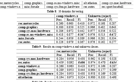
To verify the cause, we conducted more experi-ments on the 20-newsgroup data using the same setting (10 classes for test and 2 for training). The 10 classes are listed in Table 8. We show the re-sults for two sets of experiments. In each set of the experiments, we keep one known class unchanged in training and select different classes as the se-cond class. We show how the results change on the unchanged class as well as the unknown (reject)
classes. Table 9 gives the precision, recall, and F1 score for comp.windows.x and for the unknown classes. Similarly, Table 10 gives the results for rec.motorcycles and for the unknown classes. The first column in both tables are the different second classes used in training. We can see that in both sets of experiments, the precision and F1 score on the unchanged known classes (comp.windows.x and rec.motorcycles) are better when a more simi-lar class (closer in distance) is selected in training. In particular, comp.windows.x achieves the best re-sult when comp.os.ms-windows.misc is the second known class, and rec.motorcycles achieves the best result when rec.autos is the second known class. This is because the radius 𝑟! for each positively labeled space is determined based on the distance between the positive and negative training exam-ples. As related classes are closer in distance, a tighter boundary with smaller 𝑟! can be learned.
However, our results show in the cases when only 2 known classes are available, a tight boundary is harder to achieve for either class for cbsSVM.
5
Conclusion
In this paper, we proposed to study the problem of multiclass open text classification. In particular, we investigated the problem via reducing the open space risk, and proposed a solution based on cen-rec.motorcycles comp.graphics comp.os.ms-windows.misc alt.atheism comp.sys.mac.hardware comp.windows.x misc.forsale comp.sys.ibm.pc.hardware rec.autos rec.sport.baseball
Table 8: 10 domains for testing.
comp.windows.x Unknown (reject)
Prec. Recall F1 Prec. Recall F1
rec.motorcycles 0.260 0.963 0.410 0.972 0.168 0.287
comp.graphics 0.380 0.850 0.525 0.966 0.482 0.643
comp.sys.mac.hardware 0.286 0.972 0.442 0.977 0.356 0.522
comp.os.ms-windows.misc 0.418 0.877 0.567 0.976 0.513 0.672 misc.forsale 0.244 0.959 0.389 0.966 0.201 0.334
rec.autos 0.226 0.979 0.367 0.976 0.162 0.277
Table 9: Results on comp.windows.x and unknown classes.
rec.motorcycles Unknown (reject)
Prec. Recall F1 Prec. Recall F1
comp.sys.mac.hardware 0.284 0.956 0.438 0.962 0.198 0.328
rec.autos 0.459 0.892 0.606 0.974 0.470 0.634 comp.windows.x 0.260 0.963 0.410 0.972 0.168 0.287
comp.graphics 0.289 0.953 0.444 0.964 0.177 0.299
comp.sys.ibm.pc.hardware 0.284 0.953 0.438 0.958 0.169 0.288
[image:8.612.91.527.55.320.2]alt.atheism 0.194 0.973 0.324 0.980 0.333 0.498
ter-based similarity space learning. The solution reduced the positive labeled area from an infinite space to a finite space compared to previous work. This markedly reduces the open space risk. With extensive experiments across two public multiclass datasets, we demonstrated that the proposed solu-tion is highly promising. Our future work includes designing a more robust solution that still works well when the number of known classes is small.
Acknowledgments
This work was supported in part by a grant from National Science Foundation (NSF) under grant no. IIS-1407927, a NCI grant under grant no. R01CA192240, and a gift from Bosch. The content of the paper is solely the responsibility of the au-thors and does not necessarily represent the official views of the NSF, NCI, or Bosch.
References
Bravo, C., Lobato, J.L., Weber, R., L’Huillier, G. 2008. A hybrid system for probability estimation in mu l-ticlass problems combining svms and neural
net-works. In: Hybrid Intelligent Systems. pp. 649–654 Chang, C-C. and Lin, C-J. 2011. LIBSVM: a library for
support vector machines. ACM Transactions on Inte l-ligent Systems and Technology, 2:27:1--27:27,
http://www.csie.ntu.edu. tw/~cjlin/libsvm
Colas, F. and Brazdil. P. 2006. Comparison of SVM and some older classification algorithms in text classif i-cation tasks. Artificial Intelligence in Theory and
Practice. IFIP International Federation for
Infor-mation Processing, pp. 169-178.
Dalvi, B., Cohen, W. W. and Callan, J. 2013. Explorato-ry learning. In ECML.
Duan, K.B. and Keerthi, S.S. 2005. Which is the best
multiclass SVM method? An empirical study. In: Proceedings of the 6th International Conference on
Multiple Classifier Systems. pp. 278–285
Fei, G. and Liu, B. 2015. Social Media Text Classific a-tion under Negative Covariate Shift. Proceedings of
the 2015 Conference on Empirical Methods in Nat u-ral Language Processing, Lisboa, Portugal, 17-21 September.
Fumera, G., and Roli, F. 2002. Support vector machines with embedded reject option. In: International Work-shop on Pattern Recognition with Support Vector Machines (SVM2002). pp. 68–82
Hastie, T. and Tibshirani, R. 1996. Classification by pairwise coupling. In: Annals of Statistics. pp. 507– 513. MIT Press
Huang, T.K., Weng, R.C., and Lin, C.J. 2006. Genera l-ized bradley-terry models and multi-class probability
estimates. Journal of Machine Learning Research 85–115
Jain, L. P., Scheirer, W. J., and Boult, T. E. 2014. Multi -class open set recognition using probability of inclu-sion. In Proc. ECCV, pages 393-409. Springer. Jindal, N. and Liu, B. 2008. Opinion Spam and Anal
y-sis. Proceedings of the ACM Conference on Web Search and Data Mining.
Joachims, T. 1998. Text categorization with support vec-tor machines: Learning with many relevant features.
ECML.
Khan, S. and Madden, M. 2014. One-Class Classific a-tion: Taxonomy of Study and Review of Techniques. The Knowledge Engineering Review, 1-30.
Kwok, J.T.Y. 1999. Moderating the outputs of support vector machine classifiers. IEEE Transactions on
Neural Networks 10(5), 1018–1031
Manning, C. D., Prabhakar R., and Hinrich, S. 2008. I n-troduction to Information Retrieval. Cambridge Un
i-versity Press.
Shackel, N., Bertrand’s Paradox and the Principle of I n-difference. 2007. Philosophy of Science, vol. 74, no. 2, pp. 150–175.
Platt, J. C. 2000. Probabilistic outputs for support vector
machines and comparison to regularized likelihood methods. In Advances in Large Margin Classifiers, A.
Smola, P. Bartlett, B. Schölkopf, and D. Schuurmans, Eds. MIT Press, Cambridge, MA.
Rennie, J. 20-newsgroup dataset. 2008
Rocchio, J. 1971. Relevant feedback in information r
e-trieval. In G. Salton (ed.). The smart retrieval system: experiments in automatic document processing.
Scheirer, W., Rocha A., Sapkota A., and Boult T. E. Towards open set recognition. 2013. IEEE Trans.
Pattern Analysis and Machine Intelligence, vol. 36,
no. 7, pp.1757 -1772
Scheirer, W. J., Jain, L. P., and Boult, T. E. 2014. Prob
a-bility models for open set recognition, IEEE Trans.
Pattern Analysis and Machine Intelligence, vol. 36, no. 11, pp.2317 -2324
Scholkopf, B., Platt, J. C., Shawe-Taylor, J. C., Smola, A. J., Williamson, R. C. 2001. Estimating the support of a high-dimensional distribution. Neural Computa-tion 13, 1443–1471
Tax, D.M.J., Duin, R.P.W. 2004. Support vector data
de-scription. Machine Learning 54, 45–66
Vapnik, V.N. 1998. Statistical Learning Theory. Wiley -Interscience