funSentiment at SemEval 2017 Task 4: Topic Based Message Sentiment Classification by Exploiting Word Embeddings, Text Features and Target Contexts

funSentiment at SemEval-2017 Task 4: Topic-Based Message

Senti-ment Classification by Exploiting Word Embeddings, Text Features

and Target Contexts

Quanzhi Li, Armineh Nourbakhsh, Xiaomo Liu, Rui Fang, Sameena Shah

Research and Development Thomson Reuters

3 Times Square, NYC, NY 10036

{quanzhi.li, armineh.nourbakhsh, xiaomo.liu, rui.fang, sameena.shah}@thomsonreuters.com

Abstract

This paper describes the approach we used for SemEval-2017 Task 4: Sentiment Analysis in Twitter. Topic-based (target-dependent) sentiment analysis has become attractive and been used in some applications recently, but it is still a challenging research task. In our approach, we take the left and right context of a target into consideration when generating polarity classification features. We use two types of word embeddings in our classifiers: the general word embeddings learned from 200 million tweets, and sen-timent-specific word embeddings learned from 10 million tweets using distance supervision. We also incorporate a text feature model in our algorithm. This model produces features based on text negation, tf.idf weighting scheme, and a Rocchio text classification method. We participated in four subtasks (B, C, D & E for English), all of which are about topic-based message polarity classification. Our team is ranked #6 in subtask B, #3 by MAEu and #9 by MAEm in sub-task C, #3 using RAE and #6 using KLD in subsub-task D, and #3 in subtask E.

1

Introduction

There have been many studies on message or sentence level sentiment classification (Go et al., 2009; Mohammand et al., 2013; Pang et al., 2002; Liu, 2012; Tang et al., 2014), but there are few studies on target-dependent, or topic-based, sentiment prediction (Jiang et al., 2011; Dong et al., 2014; Vo and Zhang, 2015). A target entity in a message does not necessarily have the same polarity type as the message, and different enti-ties in the same message may have different po-larities. For example, in the tweet “Linux is bet-ter than Windows”, the two named entities, Linux and Windows, will have different senti-ment polarities. In this paper, we describe our approach for the subtask B, C, D & E of

SemEval-17 Task 4: Sentiment Analysis in Twit-ter (Sara Rosenthal and Noura Farra and Preslav Nakov, 2017). All the four subtasks are on top-ic-based message sentiment classification. Task B and C are about topic-based message polarity classification. Given a message and a topic, in task B, we classify the message on a two-point scale: positive or negative sentiment towards the topic. And in task C, we classify the message on a five-point scale: sentiment conveyed by the tweet towards the topic on a five-point scale. Task D and E are about Tweet quantification. Given a set of tweets about a given topic, in task D, we want to estimate the distribution of the tweets across two-point scale - the positive and negative classes, and in task E, we estimate that on a point scale - the five classes of a five-point scale. Our approach uses word embeddings (WE) learned from general tweets, sentiment specific word embeddings (SSWE) learned from distance supervised tweets, and a weighted text feature model (WTM).

SSWE encodes sentiment information in the word embeddings.

In our approach, we incorporate WE, SSWE and a weighted text feature model (WTM) togeth-er. The WTM model generates two types of fea-tures. The first type is a negation feature based on the negation words in a tweet. The second set of features is created by computing the similarity be-tween the tweet and each of the polarity types, us-ing cosine similarity and the tf.idf word weightus-ing scheme. Each polarity category is represented by a pseudo centroid tweet learned from training data. This is very similar to the Rocchio text classifier (Christopher et al., 2008), but here all the similari-ty values with all the polarisimilari-ty similari-types are used as features, and fed to the classification algorithm. The rationale behind the second set of features is that the similarity values with the different polari-ty polari-types will have some correlations, and using all of them as features will provide more information to the classifier. For example, a positive tweet usually will have a higher similarity value with neutral type than with the negative type. This will provide an additional signal to the classifier.

The context of an entity will affect its polarity value, and usually an entity has a left context and also a right one, unless it is at the beginning or end of a message. Both the context information and the interaction between these two contexts are included in the classification features of our approach. Our approach uses both SSWE and WE to represent these contexts, since WE and SSWE complement each other, and our experi-ment shows that using both increases the accura-cy by more than 6%, compared to using only one of them.

In the following sections, we present the re-lated studies, our methodology and the experi-ments and results for subtask B, C, D and E.

2

Related Work

Message Level Sentiment: Traditional sentiment classification approaches use sentiment lexicons (Mohammad et al., 2013; Thelwall et al., 2012; Turney, 2002) to generate various features. Pang et al. treat sentiment classification as a special case of text categorization, by applying learning algorithms (2002). Many studies follow Pang’s approach by designing features and applying dif-ferent learning algorithms on them (Feldman, 2013; Liu, 2012). Go et al. (2009) proposed a dis-tance supervision approach to derive features from

tweets obtained by positive and negative emo-tions. Some studies (Hu et al., 2013; Liu, 2012; Pak and Paroubek 2010) follow this approach. Feature engineering plays an important role in tweet sentiment classification; Mohammad et al. (2013) implemented hundreds of hand-crafted fea-tures for tweet sentiment classification.

Deep learning has been used in the sentiment analysis tasks, mainly by applying word embeddings (Collobert et al., 2011; Mikolov et al., 2013). Learning the compositionality of phrase and sentence and then using them in sentiment classification is also explored by some studies (Hermann and Blunsom, 2013; Socher et al., 2011; Socher et al., 2013). Using the general word embeddings directly in sentiment classification may not be effective, since they mainly model a word’s semantic context, ignoring the sentiment clues in text. Tang et al. (2014) propose a senti-ment-specific word embedding method by extend-ing the word embeddextend-ing algorithm from (Collobert et al., 2011) and incorporating senti-ment data in the learning of word embeddings. Target-dependent Sentiment: Jiang et al. (2011) use both entity dependent and independ-ent features generated based on a set of rules to assign polarity to entities. By using POS features and the CRF algorithm, Mitchell et al. (2013) identify polarities for people and organizations in tweets. Dong et al. (2014) apply adaptive recur-sive neural network on the entity level sentiment classification. These two approaches use syntax parsers to parse the tweet to generate related fea-tures. In our approach, we consider both the left and right contexts of a target when generating features.

3

Methodology

In this section, we describe the three main com-ponents used in our method, the WE, SSWE and WTM models, and how they are integrated to-gether.

3.1 Word Embedding

study to generate the WE embeddings, are the two popular word embedding models.

The embeddings are learned to optimize an objective function defined on the original text, such as likelihood for word occurrences. One implementation is the word2vec from Mikolov et al. (2013). This model has two training options, continuous bag of words and the Skip-gram model. The Skip-gram model is an efficient method for learning high-quality distributed vec-tor representations that capture a large number of precise syntactic and semantic word relation-ships. This model is used in our method and here we briefly introduce it.

The training objective of the Skip-gram mod-el is to find word representations that are useful for predicting the surrounding words in a sen-tence or a document. Given a sequence of train-ing words W1, W2, W3, . .,WN , the Skip-gram model aims to maximize the average log proba-bility





  

 

1 , 0

) | (

log 1

i m i m

n i n N

n

W W

p N

where m is the size of the training context. A larger m will result in more semantic information and can lead to a higher accuracy, at the expense of the training time. Generating word embeddings from text corpus is an unsupervised process. To get high quality embedding vectors, a large amount of training data is necessary. Af-ter training, each word, including all hashtags in the case of tweet text, is represented by a low-dimensional, dense and real-valued vector. 3.2 Sentiment-Specific Word Embedding

The C&W model (Collobert et al., 2011) learns word embeddings based on the syntactic contexts of words. It replaces the center word with a ran-dom word and derives a corrupted n-gram. The training objective is that the original n-gram is expected to obtain a higher language model score than the corrupted n-gram. The original and cor-rupted n-grams are treated as inputs of a feed-forward neural network, respectively.

SSWE extends the C&W model by incorpo-rating the sentiment information into the neural network to learn the embeddings; it captures the sentiment information of sentences as well as the syntactic contexts of words (Tang et al., 2014). Given an original (or corrupted) n-gram and the sentiment polarity of a tweet as input, it predicts a two-dimensional vector (f0, f1), for each input

n-gram, where (f0, f1) are the language model score and sentiment score of the input n-gram, respectively. The training objectives are twofold: the original n-gram should get a higher language model score than the corrupted n-gram, and the polarity score of the original n-gram should be more aligned to the polarity label of the tweet than the corrupted one. The loss function is the linear combination of two losses - loss0 (t, t’) is the syntactic loss and loss1 (t, t’) is the sentiment loss:

loss (t, t’) = α * loss0 (t, t’) + (1-α) * loss1 (t, t’)

The SSWE model used in this study was trained from massive distant-supervised tweets, collect-ed using positive and negative emotions.

3.3 Weighted Text Feature Model (WTM) WTM features: This model only uses the train-ing data set to generate features; it does not use any external lexicon or other data sources, such as embeddings learned from millions of tweets. The feature generation process is simple, fast, and effective. This model generates two types of features for each training or test tweet:

 Negation feature - the number of negation words in the tweet. This is different from other studies that add a prefix to all the words that follow the negation word, e.g. NOT xxx becomes NOT_xxx. We use the following negation words:

no, not, cannot,

rarely, seldom, neither, hardly, nor, n’t,

never



Features corresponding to the cosine

similarity values between this tweet and

the pseudo centroid tweet of each of the

polarity types.

Pseudo centroid tweet: The pseudo centroid tweet for each sentiment type is built from train-ing data, via the followtrain-ing steps:

 Tweet text is pre-processed as follow:

o all URLs and mentions are removed

o dates are converted to a symbol

o all ratios are replaced by a special symbol

o integers and decimals are normalized to two special symbols

o all special characters, except hashtags, emoticons, question marks and excla-mations, are removed

o negation words that are already used in the negation features are removed  A tf.idf value is calculated for each term in

catego-ry is treated as a document, and tf is nor-malized by its category size.

 A pseudo centroid tweet is generated for each sentiment type. We define a centroid as a vector containing the tf.idf value for each term in this category. Although we call it a “tweet”, its length is much longer than a regular tweet.

Similarity value: For each training or test tweet, its similarity with a sentiment type is calculated as follows:

 The tweet text is pre-processed using the same steps mentioned above

 A tf.idf value is calculated for each remain-ing term

 A cosine similarity is calculated between this tweet and each sentiment type.

Figure 1. The features generated from different mod-els.

3.4 Feature Generation

3.4.1 Features

Given a tweet and the target entity, eight types of features are generated based on WE, SSWE, and WTM models. They are integrated together to train the classifier. Figure 1 shows the eight types of features. Six types of features are gener-ated from WE and SSWE embeddings for a tar-get entity. Two types of features are generated from the WTM model. The red ones are SSWE embeddings, and the blue ones are WE embeddings. The subscript letter L and R refer to the left and right side of an entity, respectively. They are described below:

WEL and WER: These are the WE embeddings

for the text on the left side and right side of the target entity, respectively. In the four subtasks, occasionally, the given topic (target) is a para-phrase of the actual target entity in the tweet text, and it is not easy to match these two. In this case,

the whole tweet text is used for both the left and right contexts, and this case is handled in the same way when generating SSWEL and SSWER described below.

SSWEL and SSWER: These are the SSWE

embeddings for the text on the left side and right side of the target entity, respectively.

WE and SSWE: these are the embeddings gen-erated from the whole message text, which means they are entity independent features. We use these two features to capture the whole mes-sage, which reflects the interaction between the left and right sides of the entity.

WTM features: It has two types of features: the negation feature and the features corresponding to the cosine similarity values between the tweet and the pseudo centroid tweet of each of the po-larity types. We have described how to generate them in the previous section.

These eight types of features together capture different types of information we are interested: the entity’s left and right contexts, the interaction of the two sides, the sentiment specific word em-bedding information, the general word embed-ding information, and the sentiment affected by negation terms.

3.4.2 Text Representation from Term Embeddings

There are different ways to obtain the representa-tion of a text segment, such as a whole tweet or the left/right context of an entity, from word embeddings. In our approach, we use the concat-enation convolution layer, which concatenates the layers of max, min and average of word embeddings, because this layer gives the best performance based in our pilot experiments.

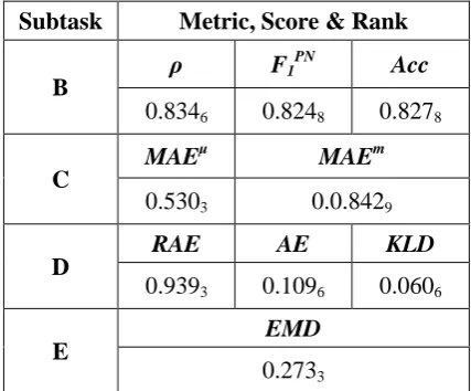
Subtask Metric, Score & Rank

B

ρ F1

PN

Acc

0.8346 0.8248 0.8278

C

MAEμ MAEm

0.5303 0.0.8429

D RAE AE KLD

0.9393 0.1096 0.0606 E

EMD

0.2733

4

Experiments and Results

4.1 WE Model Construction

The tweets for building the WE model include tweets obtained through Twitter’s public stream-ing API and the Decahose data (10% of Twitter’s streaming data) obtained from Twitter. Only English tweets are included in this study. Totally there are about 200 million tweets. Each tweet text is preprocessed to get a clean version, fol-lowing similar steps described in the WTM mod-el subsection, except the stop removal step. Stop words are not removed, since they provide im-portant information on how other words are used. Totally, about 2.9 billion words were used to train the WE model. Based on our pilot experi-ments, we set the embedding dimension size, word frequency threshold and window size as 300, 5 and 8, respectively. There are about 1.9 million unique words in this model.

4.2 SSWE Model Construction

The SSWE model for Twitter was trained from massive distant-supervised tweets (Tang et al., 2014), collected using positive and negative emoticons, such as :), =), :( and :-(. A total of 10 million tweets were collected, where 5 million contain positive emotions and the other 5 million contain negative ones. The embedding dimension size was set as 50 and the window size as 3. 4.3 Data Set and Results for Task 4

For subtask B and D, the sentiment classification and quantification based on a 2-point scale, the training data is from the related tasks of SemEval-2015 and SEmEval-2016. There are 20,538 tweets, but the actual tweet texts are not provided, due to privacy concerns. So we crawled these tweets from Twitter’s REST API. However, we were unable to obtain all these tweets because some of them were already delet-ed or not available due to authorization status change. To build our classifier, we split this data set into three parts: 70% as training data, 20% as development data and 10% for testing our classi-fier. For these two subtasks, we applied several classification algorithms, such as SMO, LibLinear and logistic regression, to see which one performs the best. The result we reported is based on logistic regression, which performed the best.

For subtask C and E, the sentiment classifica-tion and quantificaclassifica-tion based on a 5-point scale, the training data is from the related tasks of SemEval-2016. There are 30,632 tweets, and

similarly to subtask B and D, we downloaded the tweets from Twitter’s API and split them into three parts. The result we reported is based on SMO (Keerthi et al., 2001), which performed the best among several classifiers we tested. SMO is a sequential minimal optimization algorithm for training a support vector classifier.

Table 1 shows the results of our approach for the four subtasks. It lists the scores and ranks of our team for all the performance metrics used for each subtask. The subscript of each score is the rank of our team using that metric for that sub-task.

The meanings of the measures used in Table 1 are explained below:

For task B: ρ is the macro-averaged recall, which is macro-averaged over the positive and the negative class. Accuracy and F1 measures are also used for subtask B. As subtask B is topic-based, each metric is computed individually for each topic, and then the results are averaged across the topics to yield the final score. This is the same for all the measures used in task C, D and E, which are all topic based tasks.

For task C: MAEM is the macro-averaged mean absolute error, which is an ordinal classification measure. Note that MAEM is a measure of error, not accuracy, and thus lower values are better. MAEμ is an extension of macro-averaged recall for ordinal regression. More details about these two measures are described in (Baccianella et al., 2009; Nakov et al., 2016a).

For task D: KLD is the Kullback-Leibler Diver-gence measure, a measure of error, which means that lower values are better. AE is the absolute error and RAE is the relative absolute error. For task E: Subtask E is an ordinal quantifica-tion task. As in binary quantificaquantifica-tion, the goal is to compute the distribution across classes, as-suming a quantification setup. EMD is Earth Mover’s Distance (Rubner et al., 2000), which is currently the only known measure for ordinal quantification. Like KLD and MAE, EMD is a measure of error, so lower values are better.

5

Conclusion

weighted text feature model in our algorithm. Our team is ranked #6 in subtask B, #3 using MAEu metric and #9 using MAEm metric in task C, #3 using RAE and #6 using KLD in sub-task D, and #3 in subsub-task E.

References

Stefano Baccianella, Andrea Esuli , Fabrizio Sebastiani, SentiWordNet 3.0: An Enhanced Lexical Resource for Sentiment Analysis and Opinion Mining, LREC 2010

Stefano Baccianella, Andrea Esuli, and Fabrizio Sebastiani. 2009. Evaluation measures for ordinal regression. In Proceedings of the 9th IEEE Inter-national Conference on Intelligent Systems Design and Applications (ISDA 2009). Pisa, IT, pages 283–287.

Ronan Collobert, Jason Weston, Leon Bottou, Michael Karlen, Koray Kavukcuoglu, and Pavel Kuksa. Natural language processing (almost) from scratch. Journal Machine Learning Research, 12:2493–2537, 2011.

L. Dong, F. Wei, C. Tan, D. Tang, M. Zhou, K. Xu, adaptive recurisive neural network for target-depedant twitter sentiment classification. In Proceedings of ACL 2014.

R.-E. Fan, K.-W. Chang, C.-J. Hsieh, X.-R. Wang, and C.-J. Lin. LIBLINEAR: A Library for Large Linear Classification, Journal of Machine Learning Research, 9(2008), 1871-1874.

Ronen Feldman. 2013. Techniques and applications for sentiment analysis. Communications of the ACM, 56(4):82–89.

Alec Go, Lei Huang, and Richa Bhayani. 2009. Twitter sentiment analysis. Final Projects from CS224N for Spring 2008/2009 at The Stanford Natural Language Processing Group.

Karl M. Hermann and Phil Blunsom. 2013. The role of syntax in vector space models of compositional semantics. In Proceedings ACL, pages 894–904 Xia Hu, Jiliang Tang, Huiji Gao, and Huan Liu. 2013.

Unsupervised sentiment analysis with emotional signals. In Proceedings of the International World Wide Web Conference, pages 607–618.

L. Jiang, M. Yu, M. Zhou, X. Liu, T. Zhao, target-depedant twitter sentiment classification, In Proceedings of ACL 2011

S.S. Keerthi, S.K. Shevade, C. Bhattacharyya, K.R.K. Murthy, 2001. Improvements to Platt's SMO Algorithm for SVM Classifier Design. Neural Computation. 13(3):637-649.

Bing Liu. 2012. Sentiment analysis and opinion mining. Synthesis Lectures on Human Language Technologies, 5(1):1–167

Tomas Mikolov, Ilya Sutskever, Kai Chen, Greg Corrado, and Jeffrey Dean. Distributed Representations of Words and Phrases and their Compositionality. In Proceedings of NIPS, 2013. Christopher Manning, Prabhakar Raghavan and

Hinrich Schütze, (2008), Vector space classification. Introduction to Information Retrieval. Cambridge University Press.

Margaret Mitchell, Jacqui Aguilar,Theresa Wilson, and Benjamin Van Durme. Open domain targeted sentiment. I Proceedings of EMNLP, 2013. Saif M Mohammad, Svetlana Kiritchenko, and

Xiaodan Zhu. 2013. Nrc-canada: Building the

state-ofthe- art in sentiment analysis of tweets. In Proceedings of SemEval 2013.

P. Nakov, A. Ritter, S. Rosenthal, F. Sebastiani and V. Stoyanov. 2016. SemEval-2016 Tasks: Senti-ment Analysis in Twitter. In Proceedings of SemEval 2016

Alexander Pak and Patrick Paroubek. 2010. Twitter as a corpus for sentiment analysis and opinion mining. In Proceedings of Language Resources and Evaluation Conference, volume 2010.

Bo Pang, Lillian Lee, and Shivakumar Vaithyanathan. 2002. Thumbs up? sentiment classification using machine learning techniques. In Proceedings of EMNLP, pages 79–86

J. Platt, Fast Training of Support Vector Machines using Sequential Minimal Optimization. In B. Schoelkopf and C. Burges and A. Smola, editors, Advances in Kernel Methods - Support Vector Learning, 1998

Sara Rosenthal and Noura Farra and Preslav Nakov, SemEval-2017 Task 4: Sentiment Analysis in Twitter. In Proceedings of SemEval 2017, Vancouver, Canada

Yossi Rubner, Carlo Tomasi, and Leonidas J. Guibas. 2000. The Earth Mover’s Distance as a metric for image retrieval. International Journal of Computer Vision, 40(2):99–121.

Richard Socher, J. Pennington, E.H. Huang, A.Y. Ng, and C.D. Manning. 2011. Semi-supervised recursive autoencoders for predicting sentiment distributions. In Proceedings of EMNLP 2011, pages 151–161.

Richard Socher, Alex Perelygin, Jean Wu, Jason Chuang, Christopher D. Manning, Andrew Ng, and Christopher Potts. 2013. Recursive deep models for semantic compositionality over a sentiment treebank. In Proceedings of EMNLP 2013, pages 1631–1642.

Duyu Tang, Furu Wei, Nan Yang, Ming Zhou, Ting Liu, and Bing Qin. 2014. Learning sentimentspecific word embedding for twitter sentiment classification. In Proceedings of ACL 2014, pages 1555–1565.

Duyu Tang, Bing Qin, Xiaocheng Feng, Ting Liu, 2016. Effective LSTMs for Target-Dependent Sentiment Classification, In Proceedings of COLING 2016

Mike Thelwall, Kevan Buckley, and Georgios Paltoglou. 2012. Sentiment strength detection for the social web. Journal of the American Society for Information Science and Technology, 63(1):163–173.

Peter D Turney. 2002. Thumbs up or thumbs down?: semantic orientation applied to unsupervised classification of reviews. In Proceedings of ACL, pages 417–424

D. Vo and Y. Zhang, Target-dependant twitter sentiment classification with rich automatic features, IJCAI 2015.