Density estimation implications of increasing ambient noise on beaked whale click detection and classification

Density estimation implications of

increasing ambient noise on

beaked whale click

detection and classification

Tiago A. Marques

, Jessica Ward

, Susan Jarvis

, David

Moretti

, Ronald Morrissey

, Nancy DiMarzio

& Len Thomas

St Andrews, 2010

1 _{Centre for Research into Ecological and Environmental Modelling, University of}

St. Andrews, St. Andrews, Scotland, United Kingdom2 Naval Undersea Warfare

Center Division Newport, Newport, RI, USA

Contents

Abstract 3

1 Introduction 4

1.1 Available data sets . . . 4

2 Acoustic data processing 5 2.1 Measuring noise . . . 5

2.2 Adding noise . . . 7

3 Exploratory data analysis 8 3.1 Added noise DTag data set . . . 8

3.2 Ambient noise . . . 8

3.3 Detection probability as a function of range . . . 9

3.4 Detection probability as a function of added noise . . . 14

4 Detection function models 14

5 Conclusion 19

Acknowledgements 21

Abstract

Acoustic based density estimates are being increasingly used. Usually density es-timation methods require one to evaluate the effective survey area of the acoustic sensors, or equivalently estimate the mean detection probability of detecting the animals or cues of interest. This is often done based on an estimated detection function, the probability of detecting an object of interest as a function of covari-ates, usually distance and additional covariates. If the actual survey data and the data used to estimate a detection function are not collected simultaneously, as in

Marques et al. (2009), the estimated detection function might not correspond to

the detection process that generated the survey data. This would lead to biased density estimates.

Here we evaluate the influence of ambient noise in the detection and classifica-tion of beaked whale clicks at the Atlantic Undersea Test and Evaluaclassifica-tion Center (AUTEC) hydrophones, to assess if the density estimates reported in Marques

et al. (2009) might have been biased. To do so we contaminated a data set with

1

Introduction

Marques et al. (2009) presented a method for estimating the density of cetaceans

using passive acoustic detections, using as a case study a set of data on Blainville’s

beaked whale (Mesoplodon densirostris) from the US Navy AUTEC testing range

in the Bahamas. Density was estimated over a 6 day data set. One important com-ponent of the calculations is to estimate the average probability of detection of a vocalization (in this case a beaked whale click), given one is produced within some fixed distance of a study hydrophone. In their paper, Marques et. al used

auxil-iary data from animals fitted with acoustic and acceleration-sensing tags (“DTags”,

Johnson and Tyack (2003)) to estimate a “detection function” – the probability of detection as a function of distance (and other variables), and then used the esti-mated detection function to estimate average detection probability. One potential issue, noted by Marques et al. is that ambient noise might represent a source of bias in the reported density estimate. The detection function was estimated from DTag data, and it was assumed that this estimated detection function was rep-resentative of the conditions observed during the 6 day survey period. However, especially for beaked whales, DTag’s are usually only deployed in low sea-state conditions, which could result in lower background ambient noise as compared to the 6 day data set. If this is true, then the average detection probability would have been overestimated, and density underestimated.

This report presents an attempt to evaluate the influence of ambient noise on the detection and classification of beaked whale clicks and the corresponding impacts on density estimation.

Note that in Ward et al. (in press) we also looked at closely related issues.

However, there is a fundamental difference with respect to the analysis presented

here. In Ward et al. (in press) the classification stage was bypassed, in an

at-tempt to characterize the performance of the detector. So it is important to stress that while we henceforth refer just to the “detection” process, it actually corre-sponds, unless the difference is made explicit, to the joint process of detection and classification.

1.1

Available data sets

Three data sets are available for analysis. The key difference between them relates to the specific sound processing hardware used as described below:

of 6 m/s (11 knots) and 11 m/s (21 knots) to the original files. These were processed using a (Naval Undersea Warfare Center) NUWC developed tool (”wavmcast”) and do not have the higher electronic noise floor of files pro-cessed in the (Digital Signal Processing) DSP lab (see methods for details). Note we only have data from 5 unidirectional hydrophones (hydrophones 65, 66, 73 and 74 for dive 2, 66 and 67 for dive 3, and 67 for dive 4).

2. “ambient noise DTag data” - contains 9 files in total, to which no noise was added. These correspond to 9 dives, namely dives 2 and 3 from Md06 296, dives 1 to 4 from Md07 248a and dives 2 to 4 from Md07 248b. These files were processed via playback of Alesis hard disk recordings through the in-lab M3R DSP chassis and do have the noise floor issue (see methods for details).

3. “6 day ambient noise data” - a single file named “Ambient6day 16Jul10.txt” containing the ambient noise data over the 6 days data set. Note this file was also processed via playback of Alesis hard disk recordings through the in-lab M3R DSP chassis, and so is only internally consistent with the “ambient noise DTag data”.

Since we are interested in the effect of noise on detection, we only used the first data set, the only one to which noise was added. Additionally, the first set was used to avoid inconsistencies attributed to differences in processing procedures for these 3 data sets. The sole exception is in section 3.2, where some details about the other two data sets is presented.

For the estimation of the detection function in Marques et al. (2009), DTag

data from 4 whales, 13 dives were used. Here only data from 3 dives (over 1 whale) was available, and even for the dives with available data, a much smaller number of hydrophones were represented in the data set. Since a small subset of the original data were used, the same results would not be necessarily obtained, even if the same analysis was implemented.

2

Acoustic data processing

The reader is referred to Ward et al. (in press) for additional details about the

acoustic data processing.

2.1

Measuring noise

features such as waves crashing on a reef, and variations in system hardware. Extracting sound file cuts from enough hydrophones to fully represent this dynamic environment would be extremely time consuming, so consequently an alternative method of extracting ambient noise levels was developed using existing and readily available Fast Fourier Transform (FFT) detection archives.

The FFT detector implements a 2048-point FFT with 50 % overlap at a sample rate of 96 kHz on data received from the hydrophones through the onshore signal processing system. This results in a detection time resolution of 10.7 ms and a frequency resolution of 46.875 Hz over a bandwidth of 0 to 48 kHz. An indepen-dent noise-variable threshold based on a simple exponential average is run on each FFT bin. Bins that exceed the threshold are considered “detections” and set to a 1, while the remaining bins are set to 0. Detection reports which document the receiver, time of detection, maximum bin energy level, and the binary (1/0) state of each FFT bin are archived. In the absence of a signal, ambient noise in the en-vironment triggers random frequency bins resulting in “sprinkles”, defined as (false positive) detection reports, each consisting of a single positive frequency bin with a corresponding threshold level that represents the in-band noise level. Since the “sprinkles” occur randomly across the entire frequency band, these measurements can be accumulated over time to produce an ambient noise spectrum level curve over the entire frequency band. The “sprinkles” approach was shown to provide an adequate representation of the ambient noise (Ward, unpublished data).

Over the time period of interest, FFT detector “sprinkles” are accumulated over successive five minute increments. An empirical cumulative distribution function (CDF) is calculated for each 2 kHz interval. For each frequency bin the 10 % CDF value is taken as representative of the baseline ambient noise level (referred as

N L(f) in the formula below). An empirical evaluation of the data indicated that

the use of this 10% CDF value removes the effect of outliers and minimizes the likelihood of man-made noise contamination. The ambient noise spectrum (ANS)

for frequencyf is calculated as:

ANS(f) (dB re 1µP a) =N L(f) +Gain+ 10 log₁₀(2000/46.875) (1)

The low frequency (ANl) and high frequency (ANh, sometimes referred as

noise1) ambient noise criteria is the summation of spectrum levels (dB) less and greater than 24 kHz, respectively, such that:

ANl = 10 log10( 24_∑kHz

f=0

ANh = 10 log10( 48∑kHz

f=24kHz

(10ANS(f)/10)) (3)

Note in the current report we only analyze ANh, as that corresponds to the

frequency band where most of the energy from beaked whale clicks is present. The hydrophones at AUTEC have four distinct classes of hardware with cor-responding array names: Whiskey 1, Whiskey 2, Advanced Hydrophone Replace-ment Program (AHRP) Uni-directional, and AHRP Bi-directional. The Whiskey 1 and 2 arrays are extremely variable with poor documentation of gain levels; therefore, these were not analyzed. AHRP bidirectional and unidirectional hy-drophones have different response curves but similar gain values. Therefore, the following hydrophones were evaluated from the six day data set:

• AHRP Bi-directional: 15, 45

• AHRP Uni-directional: 25, 31, 34, 45, 65, 66, 67, 73, 74, 76, 80, 91.

Recall that, as stated above, this “6 day ambient noise data” is not currently considered in detail in this report.

2.2

Adding noise

The surface generated component of ambient noise is largely dependent upon wind speed. To simulate the effects of increasing surface generated ambient noise on the probability of detection, synthetic ocean noise was generated and scaled to corre-spond to the average noise level observed at wind speeds of 11 and 21 knots (5.7 and 10.8 m/s, or SS6 and SS11 in the code). The synthetic ambient noise was created by filtering white Gaussian noise using a Finite Impulse Response (FIR) filter (Jarvis, 1993) whose coefficients were determined from a year long ambient

measurements. See Ward et al. (in press) for details regarding the processing of

this year long data set. The resulting scaled synthetic noise has spectral char-acteristics representative of the year long noise average received at these higher wind speeds. This noise was then added to the baseline low noise signal. The sum was output as a wav-format file for processing through the Marine Mammal

Monitoring on Navy Ranges (M3R) detection software toolset (Morrissey et al.,

2006). This process was repeated for each combination of dive, hydrophone and

noise level (see Table 1 in Wardet al. (in press)), hence creating the added noise

3

Exploratory data analysis

3.1

Added noise DTag data set

We used data files provided by Jessica Ward on the 16th June 2010. After reading these files some minor modifications were made.

Note that the data could have been analyzed by replacing respectively every 2nd and 3rd click in the original files by the corresponding click with noise SS6 and SS11 added, or by considering multiple instances of the same click. Here, we opted by the latter option. The choice between these two approaches is likely irrelevant for the purposes of this report, as the key difference is that rather than having 3 independent measurements for each click (as the current analysis assumes) these correspond to 3 (no noise added, low noise added and high noise added) repeated measurements over each click.

In figure 1 we show the values of the original ambient noise over time, for each of the 3 dives to which noise was added. The effect of the linear interpolation on measurements made every 5 minutes is clear. In figure 2 we present the original

noise values in dB reµPa @ 1m (hereafter dB) versus the resulting noise levels when

noise (SS6 or SS11) is added. While one might have expected a priori monotonic relations between these quantities (e.g. see the relation presented for Dive 4), that seems not to not have been the case at least for dives 2 and 3. This was due to the process of measuring noise after synthetic ocean noise was added to the original files. Recall that noise had to be measured, and the measurement was not error free, as it involved averages of “sprinkles” over 5 minute periods and a linear interpolation between these.

3.2

Ambient noise

Note that the data in this section are not internally consistent with the data to which noise was added. Nonetheless, because the data processing was internally consistent, we compare here the “ambient noise DTag data” and the “6 day ambient noise data”, to see the extent to which the DTag data was in fact collected during quieter periods.

We began by reading in both data sets. Histograms for both data sets are

shown in Figure 3. A number of unusually high noise values (ANh>85) in the 6

day data set were considered as outliers and removed from the plot. The plots appear to show there is a slightly wider range of values over the six day data set, as expected given these represent a much longer time period.

The original concept was to use wind speed as a proxy for ambient noise over

21502000 21503500

57.0

57.5

58.0

58.5

Dive 2

Time (in seconds)

noise (dB)

21520000 21521000 21522000

58.0

58.5

59.0

59.5

60.0

Dive 3

Time (in seconds)

21533000 21534500

59

60

61

62

63

Dive 4

Time (in seconds)

Figure 1: Noise as a function of time, for each of the 3 dives. Each line represents a different hydrophone. For illustration, 5 minute periods are represented as dashed lines in the right panel.

considering the DTag data, and the relations are hardly what one might expect. The weather station at which wind speed was recorded may have been too far

from the hydrophones to expect a good correlation (cf. Figure 1 in Ward et al.

(in press)). Additionally, the system noise floor is necessarily masking some of the pattern.

3.3

Detection probability as a function of range

The empirical probability of detection as a function of range is shown in Figure 5. As expected, detection probability decreased as a function of increasing range.

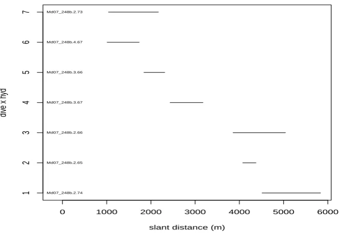
The detection range dependence on dive-hydrophone combinations is shown in Figure 6. No data were available for distances below 1 km nor between about 3.2 and 4 km. Therefore, potential inferences for those distances were ultimately unreliable, as they were necessarily based on interpolation or extrapolation.

57.0 57.5 58.0 58.5

60.4

60.8

61.2

61.6

ambient noise

SS6

57.0 57.5 58.0 58.5

63.5

64.0

64.5

65.0

ambient noise

SS11

58.0 58.5 59.0 59.5 60.0

59.7

59.9

60.1

60.3

ambient noise

SS6

58.0 58.5 59.0 59.5 60.0

63.4

63.6

63.8

64.0

ambient noise

SS11

59 60 61 62 63

60

61

62

63

ambient noise

SS6

59 60 61 62 63

64.0

64.5

65.0

65.5

ambient noise

SS11

DTag data

Frequency

60 65 70 75 80 85

0

60000

6 day data

Noise (dB)

Frequency

60 65 70 75 80 85

0

1500

Figure 3: Distribution of ambient noise in the beaked whale band (ANh) over

64 65 66 67 68 69 70

2

4

6

8

10

12

14

Ambient noise (dB)

Wind speed (m/s)

Figure 4: Ambient noise in the beaked whale band (ANh, in dB) as a function

1000 2000 3000 4000 5000

0.0

0.1

0.2

0.3

0.4

0.5

slant distance (m)

Propor

tion detected

14.412.94.16.211.34.26.55.83.2 0 0 0.48.519.84.310.15.12.41.83.1

Figure 5: Observed fraction of detected clicks (i.e. an estimate of detection probability) as a function of range. The numbers on top of the plot represent how many thousand values are used to create each data point.)

0 1000 2000 3000 4000 5000 6000

1

2

3

4

5

6

7

slant distance (m)

div

e x h

yd

Md07_248b.2.74 Md07_248b.2.65 Md07_248b.2.66 Md07_248b.3.67 Md07_248b.3.66 Md07_248b.4.67 Md07_248b.2.73

to clicks with high signal to noise ratio (SNR), i.e. typically those closer to the hydrophone (see section 4 for further details). Therefore it is not surprising that, of the above dive and hydrophone combinations, the ones for which some noise seems to increase the probability of detection are the ones which present lowest average click-hydrophone distance (note that while average distance is not on the plot, it is reflected on the overall higher detection probabilities for these two hydrophones, cf. Figure 7).

3.4

Detection probability as a function of added noise

The observed proportions of detected clicks as a function of both distance and added noise is presented in Figure 8.

The left and right panels seem to suggest that there is an initial increase in detection probability with noise at smaller distances, while the middle plot appears to show that only the highest noise level degrades detection probability. At larger distances (as shown in the left plot) adding noise seems to degrade detectability. These figures suggest that the effect of noise is really interacting with distance, but it appears that there is insufficient data, in terms of distances, to disentangle the two effects.

4

Detection function models

The reader is referred to Marqueset al.(2009) for the details regarding the GAM

model used here. A click detection probability was modeled as a function of slant

distance and vertical (vaa) and horizontal (haa) off-axis angles (angles measured

between the whale body axis and the straight line passing by the hydrophone and the whale).

As a first exploratory analysis, we assessed if clicks from a closer source seem to be more difficult to correctly classify as beaked whale (this would be the case if the classifier was misclassifying clicks from a closer sources as “delphinid”). However, neither a relatively smooth gam (k=4) nor a very wiggly gam (k=10) provide evidence for this, as the peak of the detection function in both cases is at distance 0 (Figure 9). One must bear in mind that this is a very small data set, and while that pattern was not present either in the detection function published in Marques

et al.(2009), there is some evidence in the full data set that this might actually be

the case (L. Thomas, unpublished data). This was originally suggested by Walter Zimmer (pers. comm.).

Ambient noise (dB)

Propor

tion of detected clicks

0.0 0.2 0.4 0.6

58 60 62 64

Md07_248b_Dive2

65

Md07_248b_Dive3

65

58 60 62 64

Md07_248b_Dive4

65

Md07_248b_Dive2

66

Md07_248b_Dive3

66

Md07_248b_Dive4

66

Md07_248b_Dive2

67

Md07_248b_Dive3

67

Md07_248b_Dive4

67

Md07_248b_Dive2

73

Md07_248b_Dive3

73

Md07_248b_Dive4

73

Md07_248b_Dive2

74

58 60 62 64

Md07_248b_Dive3

74

Md07_248b_Dive4

74

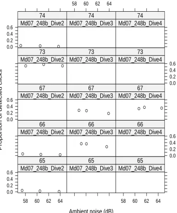
Figure 7: Proportion of detected clicks as a function of ANh, for each dive

0 2000 4000 6000 8000 0.0 0.1 0.2 0.3 0.4 0.5 0.6 Dive 2 Distance(m) Propor tion detected

0 2000 4000 6000 8000

0.0 0.1 0.2 0.3 0.4 0.5 0.6 Dive 3 Distance(m) Propor tion detected

0 2000 4000 6000 8000

0.0 0.1 0.2 0.3 0.4 0.5 0.6 Dive 4 Distance(m) Propor tion detected original SS6 SS11

Figure 8: Effect of adding noise on the proportion of detected clicks, for each of the 3 dives noise was added to.

0 2000 4000 6000 8000

0.0 0.2 0.4 0.6 0.8 1.0 Distance P(detection)

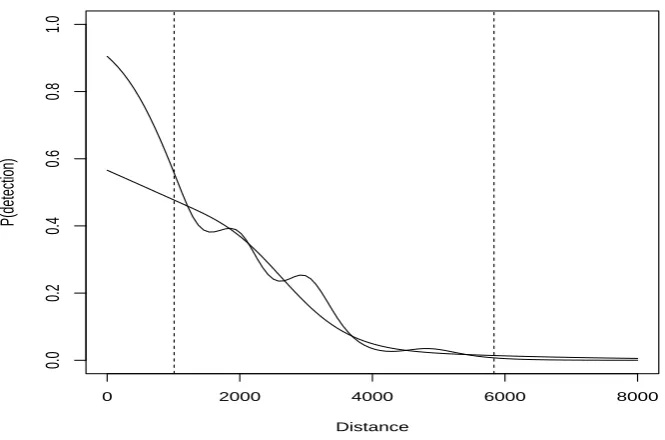
(Marques et al., 2009). Therefore that analysis was reproduced here. As shown in Figure 10, the results are very similar to those obtained previously. This suggests any differences in the models which include noise can be attributed to the effect of the noise.

We can now consider a model which also accounts for the effect of noise in detection. As shown in figure 11, there appears to be a very subtle increase in detection probability as noise increases, followed by a subtle decrease in detection probability when further noise is present. This again suggests the notion that addition of some level of noise might help the overall detection probability. We must remember that while we refer to the measure of beaked whale clicks received as a detection probability, what we model is the positive or negative outcome of a joint process of both detection and classification. What we consider to be ”a detection” (i.e. a positive event) is, in fact, a sound that is both distinguished from ambient noise and then further classified as a beaked whale click. Thus, the process used to specifically isolate the beaked whale clicks has two stages. The first stage is truly the detection part and it is applied to all acoustic data received. The FFT detector calculates a time varying threshold for each frequency bin in the FFT. The threshold is based on the exponential average of the magnitude of the energy within the bin. A broad band or click detection is declared if more than a certain number of bins within the FFT have energy which exceeds their thresholds. The number of bins required for a click detection is heuristically chosen and is currently set to 10. That is, if 10 bins in a given FFT exceed threshold then a click event has been detected. Clicks are then coarsely classified based on their frequency content. The frequency segmentation classifier has 5 bands which correspond to the bands containing peak energy for various species. Specifically, beaked whale clicks are known to have most of their energy concentrated in band from 24-48 KHz. The frequency segmentation rule for beaked whales requires that the majority of bins above threshold for a detected click are in the 24-48KHz band and that no more than 5% of the frequency bins below 24 KHz have energy above threshold. In high signal-to-noise ratio situations, such as at close ranges or in very low sea state, many beaked whale clicks have sufficient energy detected below 24 kHz that they

fail the<5% criteria. As a result, these clicks are misclassified as another species

(e.g. as a delphinid). The addition of a small amount ambient noise decreases signal-to-noise ratio more significantly at frequencies below 24 kHz, due to the fact at frequencies greater than 24 kHz the FFT detector tends to be limited by the system electrical noise floor rather than ambient noise. This results in a masking of the portion of the beaked whale click energy below 24 kHz. Thus, a portion of

these loud, close range clicks now begin to meet the<5% criteria and are correctly

0 2000 4000 6000 8000 0.0 0.2 0.4 0.6 0.8 1.0 Distance P(detection)

−3 −2 −1 0 1 2 3

−1.5 −0.5 0.5 1.0 1.5

response

0.55

1000 2000 3000 4000 5000

−3 −2 −1 0 1 2 3

response

1000 2000 3000 4000 5000

−1.5 −0.5 0.5 1.0 1.5

response

resulting probability of detection decreases with decreasing signal-to-noise ratio as expected.

Evaluating the detection function considering all the DTag data (13 dives and tens of hydrophones), rather than the currently available 3 dives and 5 hy-drophones, would likely help to understand further the influence of ambient noise on detection. Nonetheless, the fact that the 3 data sets reported here are not internally consistent prevents that analysis at this point. As an example, it was not clear from the model fit to the data presented here or the equivalent model

presented in Marqueset al.(2009) that the detection probability decreases for high

SNR (i.e. close) clicks. On the other hand, it is also not clear whether if mea-surement error associated with noise (cf. figure 2) is making it difficult to extract patterns from the data. It seems like the actual numerical values obtained after noise is added are severely constrained by the measurement error coupled with the linear interpolation. This leads to long sequences of clicks with decreasing noise in the original files which end up with increasing noise values once noise is added to them, which is clearly counter intuitive and a by-product of the analysis.

5

Conclusion

The main conclusion of this report is that while there may be an effect of ambient noise on detection probability, that effect is fainter than one might expect a priori.

The hydrophones used are very deep (>1.5 km), and therefore ambient noise suffers

considerable attenuation before reaching the hydrophones. As shown in section 3.2, for the ambient noise measures used here, there was a very small difference between the noise observed during the 6 day data set and the DTag data.

As stated above, the added noise data set analyzed here was processed using

the program wavmcast. On the other hand, the data used in Marqueset al.(2009)

was processed using the Alesis ”system” rather than wavmcast, which means that the effect of noise will be even less than that reported here. This is because the dynamic range of the Alesis output extends below the dynamic range of the M3R DSP chassis input Analog to Digital Converters, resulting in a higher electronic noise floor in the data reprocessed from the Alesis. At higher frequencies, like those of the beaked whale click, the ambient noise spectrum drops below the noise floor such that changes in the measured ambient noise are not noticeable until the added noise level rises above the electronic noise floor. Therefore the effect of added ambient noise would also be masked by the higher noise floor resulting in a less pronounced effect of increasing ambient noise on beaked whale probability of detection.

0 2000 4000 6000 8000 0.0 0.2 0.4 0.6 0.8 1.0 Distance P(detection)

1000 2000 3000 4000 5000

−3 −2 −1 0 1 2 3

response

1000 2000 3000 4000 5000

−1.5 −0.5 0.5 1.0 1.5

response

58 60 62 64 66

1000 3000 5000

response

(2009), warning against the potential impact of ambient noise in the density re-sults, may have been just over cautious. This is not to say that under different scenarios ambient noise might not be an important covariate in explaining

detec-tion probability. An example is given by Marques et al. (in press).

Acknowledgements

This report was created within the efforts of the DECAF (Density Estimation for Cetaceans from passive Acoustic Fixed sensors) project. DECAF was selected for funding under the National Oceanographic Partnership Program, a body that coordinates research initiatives among US federal and industrial partners. The partners funding our project are the Ocean Acoustics Program of the US National Marine Fisheries Service Office of Protected Resources and the Joint Industry Program. We thank Walter Zimmer’s insight, raising the issue that close by high SNR clicks were likely being misclassified by the FFT detector.

References

Jarvis, S. (1993). Signature simulation (SigSim) system: Development and capa-bilities. Technical report, NUWC-NPT Technical Report 10,224 (UNCLASSI-FIED).

Johnson, M. P. and Tyack, P. L. (2003). A digital acoustic recording tag for

measuring the response of wild marine mammals to sound. IEEE Journal Of

Oceanic Engineering,28, 3–12.

Marques, T. A., Thomas, L., Ward, J., DiMarzio, N., and Tyack, P. L. (2009). Estimating cetacean population density using fixed passive acoustic sensors: an

example with Blainville’s beaked whales. The Journal of the Acoustical Society

of America,125, 1982–1994.

Marques, T. A., Munger, L., Thomas, L., Wiggins, S., and Hildebrand, J. A. (in

press). Estimating North Pacific right whale (Eubalaena japonica) density using

passive acoustic cue counting. Endangered Species Research.

Morrissey, R. P., Ward, J., DiMarzio, N., Jarvis, S., and Moretti, D. J. (2006).

Passive acoustic detection and localization of sperm whales (Physeter

macro-cephalus) in the tongue of the ocean. Applied Acoustics,67, 1091–1105.

Ward, J., Jarvis, S., Moretti, D., Morrissey, R., DiMarzio, N., Thomas, L., and

detection with increasing ambient noise. The Journal of the Acoustical Society