Luis A. Correa,1,∗ Mohammad Mehboudi,1 Gerardo Adesso,2 and Anna Sanpera3, 1 1Departament de F´ısica, Universitat Aut`onoma de Barcelona - E08193 Bellaterra, Spain
2School of Mathematical Sciences, The University of Nottingham, University Park, Nottingham NG7 2RD, UK 3Instituci´o Catalana de Recerca i Estudis Avan¸cats - E08011 Barcelona, Spain
(Dated: April 21, 2015)
The unknown temperature of a sample can be estimated with minimal disturbance by putting it in thermal contact with an individual quantum probe. If the interaction time is sufficiently long so that the probe thermal-izes, the temperature can be read out directly from its steady state. Here we prove that the optimal quantum probe, acting as a thermometer with maximal thermal sensitivity, is an effective two-level atom with a maxi-mally degenerate excited state. When the total interaction time is insufficient to produce full thermalization, we optimize the estimation protocol by breaking it down into sequential stages of probe preparation, thermal contact and measurement. We observe that frequently interrogated probes initialized in the ground state achieve the best performance. For both fully and partly thermalized thermometers, the sensitivity grows significantly with the number of levels, though optimization over their energy spectrum remains always crucial.
PACS numbers: 06.20.-f, 03.65.-w, 03.65.Yz
INTRODUCTION
With the advent of quantum technologies, the study of the thermodynamics of quantum devices has attracted consider-able attention [1, 2]. In particular, there is a growing interest in obtaining accurate temperature readings with nanometric spatial resolution [3–5], which would pave the way towards many ground-breaking applications in medicine, biology or material science. This motivates the development of precise quantum thermometric techniques.
Recent progress in the manipulation of individual quan-tum systems has made it possible to use them as tempera-ture probes, thus minimizing the undesired disturbance on the sample. Fluorescent thermometry may be implemented, for instance, on a single quantum dot to accurately estimate the temperature of fermionic [6, 7] and bosonic [8, 9] reservoirs. Similarly, the ground state of colour centres in nano-diamonds has already been used as a fluorescent thermometer [3–5], achieving precisions down to the millikelvin scale, and a spa-tial resolution of few hundreds of nanometers. Thermometry applied to micro-mechanical resonators [10–12], and nuclear spins [13] has also been subject of investigation. Other studies have focused on more fundamental questions such as the scal-ing of the precision of temperature estimation with the number of quantum probes [14], and the potential role played by co-herence and entanglement in simple thermometric tasks [15].
In this Letter, we investigate the fundamental limitations on temperature estimation with individual quantum probes. Two complementary scenarios are considered. In the first one, we assume that the thermometer reaches thermal equilibrium with the sample. We then determine which are the optimal probes that maximize the attainable precision in the estima-tion of the temperature. Alternatively, we also consider the situation in which the probe does not thermalize completely due to some constraint on the total estimation time (e.g. the sample may be unstable). In this second scenario, we analyze the dissipative time evolution of the probe in order to optimize
the thermometric protocol. We model it as sequence of steps of preparation, thermal contact and readout.
Our main results are the following. First, we show that a
N-dimensional equilibrium probe with maximumheat capac-ityis optimal for thermometry. This is an effective two-level probe with (N−1)-degeneracy in the excited state, and some optimal gap. The maximum achievable precision grows with the dimension of the probe, yet the range of temperatures for which it operates efficiently as a thermometer becomes nar-rower. In contrast, a less sensitive probe with equispaced en-ergy spectrum, such as a quantum harmonic oscillator, fea-tures wider operation ranges. On the other hand, when the estimation time is limited, we find that a frequently measured probe initialized in its ground state achieves the largest ther-mal sensitivity. In this case, the overall precision still scales with the dimension of the probe, even though the temperature range for efficient operation is dimension-independent.
Our results contribute not only to the theoretical advance of temperature estimation in the quantum regime, but also have potential technological impact for the development of high precision thermometry at the nanoscale.
FULLY THERMALIZED THERMOMETERS
In standard thermometry, a (sufficiently small) thermometer is simply allowed to equilibrate with the sample to be probed, so that the temperature of the latter is inferred from the state of the probe. In a quantum scenario, the same procedure can be applied. A first approximation to the sample temperature can be obtained by performing a suitable measurement on the steady state of the thermalized probe. If a large numberνof such independent experiments is carried out, one can refine the estimateT of the sample temperature. Its corresponding uncertainty∆T is bounded from below by a geometric quan-tityF( ˆ%T), known as quantum Fisher information (QFI) [16],
via the quantum Cram´er-Rao inequality [17, 18]
∆T ≥[νF( ˆ%T)]−1/2. (1)
In the present context of temperature estimation, the QFI can be interpreted as the infinitesimal distance, according to the Bures metric, between a thermal state at temperatureT, and a thermal state at temperatureT +δ[18]. Intuitively, the more such a distance, the more the initial probe state is sensitive to a small variation of temperature. Formally,
F( ˆ%T)=−2 lim δ→0∂
2
F( ˆ%T,%ˆT+δ)/∂δ2, (2)
whereF( ˆ%1,%ˆ2) ≡
tr
q p
ˆ %1%ˆ2
p
ˆ %1
2
is the Uhlmann fidelity between states ˆ%1and ˆ%2, which defines their respective Bures distance viadBures( ˆ%1,%ˆ2) =2 1−
p
F( ˆ%1,%ˆ2)[18]. Further to the intuitive meaning of the QFI, we note that there exists an optimal estimator (i.e., an optimal measurement procedure on the final thermalized state) for which the bound in eq. (1) becomes tight for an asymptotically large number of measure-ments (ν1), and can be indeed saturated by means of adap-tive metrological schemes [16]. Therefore, the inverse of the QFI equivalently defines the minimum achievable variance in the estimation ofT. We will then refer toF(%T) as ‘thermal
sensitivity’, and take its maximization as synonym of optimal-ity in the following analysis [8–11, 14, 19].
We write the Hamiltonian of our probe as Hˆ =
P
nn|ni hn|. A thermalization process leads to stationary
states of the form ˆ%T =Pnpn|ni hn|, where the populations
are pn ≡ Z−1e−n/kBT and the partition function is given by
Z≡tre−Hˆ/kBT. In what follows we set
~=kB=1.
In the energy eigenbasis, eq. (2) rewrites as [20]
F( ˆ%T)=4
X
m,npm
| hm|∂T%ˆT|ni |2
(pm+pn)2 = ∆Hˆ2
T4 , (3)
were ∆Hˆ2 ≡ hHˆ2i − hHˆi2. In this last step, we have used the identityhHˆi=T2∂TlnZ. Interestingly, in the single shot
scenario ofν=1, one can combine eqs. (1) and (3) to get the thermodynamic uncertainty relation ∆T
T2∆Hˆ ≥ 1. Also, note
that∆Hˆ2/T2 =dhHiˆ /dT ≡C(T) which, in the present case, may be referred to as the ‘heat capacity’ of the probe. It thus follows that the signal-to-noise ratioT/∆T is upper-bounded as (T/∆T)2 ≤ C(T) [21]. Note as well that, since ˆ%
T is a
thermal state, the most informative measurement saturating eq. (1) is just a projection onto the energy eigenbasis.
In the light of eq. (3), the maximization of the thermal sen-sitivity of a probe translates into finding the energy spectrum with the largest possible energy variance at thermal equilib-rium, or equivalently, the N-dimensional probe with largest heat capacity. Note that the heat capacity of the sample must be anyway much larger than that of the probe so as to mini-mize any disturbance arising from the estimation procedure.
For a generalN-level probe, the energy variance writes as ∆Hˆ2 =Z−1PN
i
2
ie
−i/T−(Z−1PN
i ie−i/T)2, where the
parti-tion funcparti-tion isZ = P
ie−i/T. The variance is bounded. In
2 4 6 8 10
0.0 0.2 0.4 0.6 0.8 1.0
0 5 10 15 20 25 30 35
T
ℱ
0 0.5 1
0 0.5 1
T
ℱ
/
[image:2.612.339.538.51.163.2]ℱmax
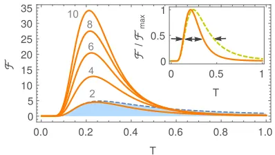
FIG. 1: QFI versus sample temperature for optimizedN-dimensional probes (orange) withN={2,4,6,8,10}. The dashed blue line repre-sents the QFI of a harmonic probe and the shaded blue area is the do-main reachable by finite-dimensional probes with equispaced spec-trum. In the inset, the normalized sensitivities of two probes with
N=2 (dashed green) andN=10 (solid orange) are compared. The arrows indicate the width of the specified temperature range. Tem-perature and QFI are both expressed in arbitrary units andΩ =1.
order to identify its maximum, we impose∂i∆H
2=0, which results in a set ofNtranscendental equations. Subtracting the
j-th equation from thei-th one (∂i∆Hˆ2−∂ j∆Hˆ
2=0), we ar-rive at the condition (i−j)(i+j−2−2hHiˆ /T)=0 (see [22]
for details). That is, any two energy eigenvaluesiandjmust
be either equal, or sum up to the same value at the stationary points of∆Hˆ2. This may only happen if the energy spectrum is that of an effective two-level atom with energies {−, +}, andN0andN−N0times degenerate ground and excited state, respectively. Without loss of generality, we may always shift the energy spectrum so that− = 0 and the optimal gap be-comes x∗N,N
0 ≡ Ω
∗/T = (
++−)/T = 2(1+hHˆi/T) > 2,
since nowhHˆi > 0. This critical gap may be conveniently rewritten asex∗N,N0 = N−N0
N0
x∗ N,N0+2
x∗ N,N0−2
. Observing that the diff er-ence∆Hˆ2(x∗
N,N0−1;N,N0−1)−∆
ˆ
H2(x∗
N,N0;N,N0)=
1 4(x
∗2
N,N0−1−
x∗N2,N
0) is always positive, one can conclude that the
excited-state degeneracy must be the largest possible (i.e.N0 =1) so as to maximize the energy variance.
Finally, to ensure that∆Hˆ2reaches a maximum atx∗
N,N0, we
must check that the Hessian matrix (Hi j ≡∂2∆Hˆ2/∂
i∂j) is
negative definite in that configuration. After a tedious but oth-erwise straightforward calculation, we can see that it hasN−2 identical eigenvaluesλ1=−12
x∗ N,1−2
N−1 , plus two non-degenerate ones: λ2 = −18
x∗2
N,1−4
N−1 andλ3 = 0. Since x ∗
N,1 > 2, bothλ1 andλ2are negative. The single vanishing eigenvalueλ3 sim-ply reflects the obvious symmetry of∆Hˆ2 with respect to a global shift of all energy levels. Hence, one may rigorously conclude that the effective two-level configuration described above indeed maximizes the energy variance. Note that this is in agreement with [23].
Here is the final expression for the corresponding QFI
FN = x
4ex
Ω2
N−1
plot eq. (4) for different values ofN. The precision in tem-perature estimation improves significantly by increasing the dimensionalityNof the probe, albeit at the expense of reduc-ing the specified temperature range for efficient operation of the probe as a thermometer (see inset of fig. 1).
So far, we have seen that the best thermometers are effective two-level atoms with a highly degenerate excited state and a specific, temperature-dependent gap. However, these may be very hard to prepare in practice, especially due to the fact that the sample temperature must be known precisely. For this rea-son we now consider more versatile sub-optimal probes with a richer spectrum, such as a single thermalized harmonic oscil-lator. In this case, the corresponding QFI can be easily com-puted from the 2×2 steady-statecovariance matrix[24, 25] of a thermal stateσT =coth2ΩT12as in eq. (2). Using the fact that the Uhlmann fidelity between two single-mode Gaussian statesσ1andσ2is given byF(σ1,σ2)=2
√
∆ + Λ− √
Λ−1
[26], where∆≡det(σ1+σ2) andΛ≡det(σ1−1)det(σ2−1), one arrives atFho= Ω
2
4T4 csch
2Ω
2T. This is represented in fig. 1
with a dashed blue line. For ease of comparison we take the oscillator frequencyΩto be+−−. As we can see, a har-monic probe features a thermal sensitivity similar to that of a two-level probe. Even if harmonic thermometers are outper-formed by most optimizedN-level probes, they are endowed with a much broader specified temperature range for efficient operation, making them a choice of practical interest. This can be understood by observing that the thermal sensitivity of a probe with a single energy gap may only peak at one charac-teristic frequency, while with an equispaced, unbounded spec-trum there will always be some transition close to resonance.
PARTLY THERMALIZED THERMOMETERS
All the previous analysis holds regardless of the probe-sample interactions or the spectral properties of the probe-sample, as long as thermalization takes place. In practice, however, one may have to read out the temperaturebeforeattaining full thermalization. This would be the case, for instance, if the sample was unstable and existed only for times comparable to the dissipation time scale. In this alternative scenario, we ask ourselves about the optimal breakup of the total running time of the estimation procedure (ts) into sequential stages
of probe-preparation, thermal contact (during time ∆t), and measurement, so as to optimize the achievable precision in eq. (1). Note that the number of interrogations is now limited toν=ts/∆t, so that the figure of merit to be maximized is the ratioF(∆t)/∆t[27, 28].
Since we must monitor the time evolution of the probe, it is necessary now to specify the sample and its coupling with the thermometer. We shall model the sample as a bosonic heat bath, linearly coupled to an arbitrary probe. The to-tal Hamiltonian writes as ˆHtot = Hˆ +Pµωµ bˆ†µbˆµ + Xˆ ⊗
P
µgµ(ˆbµ+bˆ†µ), where ˆbµis the annihilation operator of mode ωµin the sample. We choose the probe-sample coupling con-stants to be gµ = (γωµ)1/2, implying flat spectral density
J(ω) ∼ P
µ g
2
µ
ωµδ(ω−ωµ) = γ[29]. This sets the time-scale τD ∼ γ−1 over which ˆ%(t) varies appreciably. Tracing out
the sample from the overall unitary dynamics and assuming a thermal state ˆχTfor it, leads to an effective equation of motion
of the Lindblad-Gorini-Kossakovski-Sudashan type (LGKS) [30, 31], that follows from ˙ˆ% =trSdtd{e−i
ˆ
Htott%ˆ(0)⊗χˆ
T ei
ˆ
Htott},
after sequentially performing the Born, Markov and rotating-wave approximations (see [32] for a detailed derivation). Note that the Born approximation implies that no correlations are ever created between probe and sample, so the latter remains undisturbed throughout the estimation procedure. Note also that, for consistency with the Markov approximation, the tem-perature of the sample may be not arbitrarily low, as the ther-mal fluctuations must remain fast compared withτD.
In the interaction picture, the master equation can be cast as
˙ˆ %= ΓΩ,T
ˆ
AΩ%ˆAˆ−Ω−12{Aˆ−ΩAˆΩ,%ˆ}+
+e−Ω/TΓΩ,T
ˆ
A−Ω%ˆAˆΩ−12{AˆΩAˆ−Ω,%ˆ}+
, (5)
where ˆA±Ω stands for the relaxation/excitation operator as-sociated with the decay channel at frequencyΩ. These fol-low from the decomposition of ˆX =P
ωAˆω as sum of eigen-operators of the probe Hamiltonian (i.e. such that [ ˆH,AˆΩ] =
−ΩAˆΩ). It is easy to show that the thermal state ˆ%=Z−1e−Hˆ/T
is a fixed point of eq. (5) and, choosing a suitable coupling op-erator ˆX, the open dynamics may also beergodic, thus even-tually bringing any initial state to thermal equilibrium [32].
For a two-level thermometer with Hamiltonian ˆH = Ω2σˆz,
we can take, for instance, ˆX = σˆx from which ˆAΩ = |−Ω/2i hΩ/2|, while ˆA−Ω = Aˆ†Ω. Here, |±Ω/2i are the cor-responding energy eigenstates. Generalizing to the case of anN-level probe with eigenstates{|ii}, a coupling term like
ˆ
X=P
i,1|1i hi|+|ii h1|would also thermalize any prepara-tion, where we have labelled the ground state by|1i. The re-sulting relaxation operators are ˆAi−1 =|1i hi|. In particular,
to account for our effective two-level systems with excited-state degeneracy we can take the limit i → Ω2 for i , 1
and set1 = −Ω2 to get the desired thermalization process. Let us finally comment on the decay ratesΓΩ,T, which follow
from the power spectrum of the bath auto-correlation function
hSˆ(t) ˆS(0)iT ≡tr{Sˆ(t) ˆS(0) ˆχT}, where ˆS ≡Pµgµ(ˆbµ+bˆ
† µ). In the specific case of a quantum probe coupled through dipole interaction to the quantized electromagnetic field in three di-mensions, one obtainsΓΩ,T =γΩ3(1−e−Ω/T)−1[32].
2 4 10
1 10 100
0.51 5 10 50 100
Δ t
10
3
ℱ
(
Δ
t
)/
Δ
[image:4.612.81.274.51.159.2]t
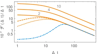
FIG. 2: Log-log plot ofF/∆tas a function of∆tfor different
prepara-tions and probe dimensionalities. The continuous orange lines stand forFNfor probes withN ={2,4,10}initialized in the ground state.
The dashed and dotted orange curves stand for a two-level probe ini-tialized in a thermal state at temperature 0.8 and 0.9, respectively. The dot-dashed blue curve corresponds to a two-level probe prepared in the maximally coherent state ˆ%(0)=|+i h+|(Ω/T =x˜,γ=10−3, andT =1, in arbitrary units).
Thus, by choosing ˆ%(0) =|−Ω/2i h−Ω/2|we can combine eqs. (5) and (3) to computeF2(∆t) as a function of the inter-rogation time∆t, starting from a ground state preparation:
F2(∆t)=
x2
ex
e∆t/τ−1
+(1+ex)∆t
2τcsch
x
2
2
(1+ex)2 e∆t/τ−1 1+exe∆t/τT2 , (6)
whereτ−1 ≡ γΩ3cothx
2. Eq. (6) shows that the details of the thermal fluctuations of the sample, encoded inΓΩ,T, only
enter in the dynamics through the scaling factorτ. Hence, even if our choice of a flat spectral density might seem pretty restrictive at first, changing the probe-sample coupling would just amount to a suitable rescaling of time.
In fig. 2 we plotF2(∆t)/∆tfor different preparations. As we can see, the sensitivity of a cold thermal probe peaks at some optimal readout time, after which it must be quickly cooled down to start over another relaxation stage in the estimation protocol. In the limiting case of a ground-state preparation, the overall maximum sensitivity is approached as∆t→0.
Eq. (6) can be generalized to any of our highly degenerate effective two-level probes prepared in the ground state. As before, their maximum precision follows from the limit
lim
∆t→0
FN(∆t) ∆t =
γT(N−1)x5e2x
(ex−1)3 . (7)
We now search for the optimal frequency-to-temperature ra-tio ˜xthat sets an ultimate upper bound on the thermal sen-sitivity in eq. (7). This can be expressed implicitly as ex˜ =
(5+2 ˜x)/(5−x˜), which is independent ofN. Interestingly, the specified temperature range for efficient operation does not scale withN, at variance with the fully thermalized case.
For completeness, we examine again here the performance of harmonic probes. Going back to eq. (5), we will set
ˆ
H = Ωaˆ†aˆ and ˆX =aˆ+aˆ†, whose corresponding relaxation and excitation operators are trivially ˆAΩ = aˆ and ˆA−Ω =aˆ†. The total Hamiltonian is thus quadratic in positions and mo-menta and therefore, any Gaussian preparation will preserve
its Gaussianity in time [24]. Provided that the initial state also has vanishing first order moments (hxiˆ =hpiˆ =0), its covari-ance matrixσ(t) alone will be enough for a full description.
In this case, the dynamics may be obtained by explicitly solving the quantum master equation in phase space, to yield
σ(t) =e−ΓΩ,Ttσ(0)+(1−e−ΓΩ,Tt)σ
T [24, 37]. Computing the
transient QFI is thus straightforward by resorting to eq. (2). In what follows, we shall consider general (undisplaced) single-mode Gaussian states as initial preparations; these can be writ-ten as rotated, squeezed thermal states [24, 25]. As it could be expected, ground-state initialization ( ˆ%(0) = |0i h0|) pro-vides once again the largest thermal sensitivity. One can ig-nore the temperature dependence of ΓΩ,T in the solution to
the master equation and still get a good approximation to lim∆t→0Fho(∆t)/∆t. Surprisingly, we recover eq. (7) with
N = 2. Indeed, this equivalence of two-level probes and harmonic thermometers extends generally beyond the limits ∆t → 0 and ˆ%(0) = |0i h0|. Therefore, at variance with the fully-thermalized scenario, the specified temperature range of both oscillators andN-level probes in an effective two-level configuration is virtually the same, regardless ofN.
CONCLUSIONS
We have analyzed the performance and ultimate limitations of individual quantum probes for precise thermometry on a sample. Our study is based on techniques of parameter esti-mation [16, 18], and makes use of the quantum Fisher infor-mation as indicator of optimal thermal sensitivity.
First, we have considered a general N-dimensional quan-tum probe that fully thermalizes with the sample. We have linked the quantum Fisher information with the heat capacity of the probe, and proven that the best quantum thermometer is an effective two-level atom with a maximally degenerate ex-cited state at a specific energy gap, depending non-trivially on the sample temperature. There exists a complementary trade-offbetween the maximum achievable estimation preci-sion, which grows withN, and the specified temperature range in which the estimation is efficient, which shrinks withN.
We have also considered the scenario in which, e.g. due to short lifetime of the sample, full thermalization may not take place. Frequently interrogated probes prepared in their ground state then provide the largest thermal sensitivity. While the maximum achievable precision scales again withN, the spec-ified temperature range is dimension-independent in this case. These results were obtained by considering a large bosonic sample in thermal equilibrium, weakly coupled to the probe through a linear interaction term, ensuring ergodicity. It would be interesting to discuss to which extent can the estimation precision be enhanced with a suitably engineered thermal cou-pling, e.g. by externally controlling the scattering length in a cold atomic gas [38]. In principle, this would allow the exper-imenter to directly manipulate the scaling factorτin eq. (6).
linked to the overall maximization of the precision, the poten-tial role played byquantumness in thermometry remains an open problem [13, 15] that deserves a study on its own.
The authors would like to thank J. Calsamiglia, J. Filgueiras, T. Bromley and M. Cianciaruso for fruitful discus-sions, and K. Hovhannisyan for making us aware of ref. [23] after completion of this work. Financial support from Span-ish MINECO (FIS2008-01236), EU Collaborative Project TherMiQ (Grant Agreement No. 618074), European Re-gional Development Fund, COST Action MP1209, Gener-alitat de Catalunya (Grant No. SGR2014-966), Brazilian CAPES (Grant No. 108/2012), Foundational Questions
In-stitute (Grant No. FQXi-RFP3-1317), and ERC StG GQCOP (Grant Agreement No. 637352) is acknowledged.
Details on the proof of the optimality of the effective two-level probes
Below, we give further details on the proof of the optimality of effective two-level thermalized probes with N −1 times degenerate excited state, for the maximization of the energy variance. For anN-level probe in a thermal state, this writes as
∆Hˆ2({
i})=hHˆ2i − hHiˆ 2=Z−1 N
X
i=1
2
ie
−i/T−
Z
−1
N
X
i=1
ie−i/T
2
, (8)
whereZ=P
ie−i/T. In order to find the stationary points of∆Hˆ2({i}) we simultaneously impose theNconditions∂i∆Hˆ 2({ε
i})=
0, which result in the following system of transcendental equations
e−i/T
Z
"
1
T
hHˆ2i −2hHˆi2
+i
2−i T
+2hHˆi
i T −1
#
=0 ∀i∈ {1,· · · ,N}. (9)
One may now subtract the j-th of such equations from thei-th one, obtaining
(i−j)
h
i+j−2
hHiˆ +Ti=0. (10)
That is, the stationary points of∆Hˆ2are such that any two en-ergy eigenvalues must be either equal or sum up to 2hHiˆ +T.
A set of conditions like eq. (10) cannot be simultaneously met by more than two different energy eigenvalues{+, −}. Hence, the only energy spectra compatible with stationarity are those of effective two-level atoms with ground state degeneracyN01 and anN−N0 times degenerate excited state. Without loss of generality, we may always shift the spectrum so as to set − = 0. According to eq. (10), the gap of the effective two-level system becomesΩ∗≡
+−−=2 hHiˆ +T.
Note that for an effective two-level probe the average en-ergy rewrites as
hHˆ(x;N,N0)i=T
(N−N0)x e−x
N0+(N−N0)e−x
, (11)
where we have introduced the notation x ≡ Ω/T for the frequency-to-temperature ratio (recall that we work in units of ~ = kB = 1). The energy gap at stationarity can be thus conveniently cast as
ex ∗
N,N0 = N−N0
N0
x∗
N,N0+2
x∗N,N
0−2
. (12)
In order to determine the ground and excited state de-generacies yielding the largest energy variance at the critical frequency-to-temperature ratio, we can compare ∆Hˆ2(x∗
N,N0;N,N0) with∆
ˆ
H2(x∗N
0−1,N;N,N0−1), where
∆Hˆ2(
x;N,N0)=T2
N0(N−N0)x2ex [(N−N0)+N0ex]2
. (13)
This yields ∆Hˆ2(x∗N,N
0−1;N,N0 −1) −∆
ˆ
H2(x∗N,N
0;N,N0) =
1 4(x
∗2
N,N0−1−x
∗2
N,N0)>0, which is positive according to eq. 12.
Hence, an effective two-level probe with maximally degener-ate excited stdegener-ate (i.e. N0 =1) has the largest energy variance at stationarity.
All that is left is to prove that such stationary point is in-deed a maximum for the energy variance. For that purpose, we shall compute explicitly the elements of the Hessian ma-trixHi j ≡ ∂2∆Hˆ2/∂
i∂j and check its eigenvalues for
Hii= ∂2∆Hˆ2
∂2
i
= e−i/T
Z T
!2 h
2 hHˆ2i −3hHiˆ 2−4ThHi −ˆ T2+8(T+hHiˆ )
i−4i2
+Z ei/T 2T2+2hHiˆ 2T +hHiˆ − hHˆ2i −2 2T +hHiˆ
i+i2
i ∀i∈ {2,· · ·,N}, (14)
while the off-diagonals are given by
Hi j= ∂
2∆Hˆ2
∂i∂j
=e−(i+j)/T
T2Z2
h
4hHiˆ (i+j−2T)+(i+j)(4T−i−j)+2hHˆ2i −6hHiˆ 2−2T2
i
∀i, j. (15)
We are interested in the particular case of an effective two-level spectrum withN−1 times degenerate excited state at the corresponding optimal gapx∗ ≡x∗
N,1. For this configuration, the Hessian has the following structure
H =
a c c · · · c c b d · · · d c d b · · · d
..
. ... ... ... ... c d d · · · b
, (16)
where a = Hii|i=0, b = Hii|i=x∗, c ≡ Hi j|i=0,j=x∗ =
Hi j|
i=x∗,j=0 and d = Hi j|i=j=x∗. To compute these ele-ments from eqs. (14) and (15) we can also make the follow-ing replacements Z = 2x∗/(2+x∗), hHˆi = T
2(x
∗−2) and
hHˆ2i=T22x∗(x∗−2) andex∗
=(N−1)xx∗∗+−22., yielding
a=−1
8(x ∗2−
4) (17a)
b=−(x
∗−2)(4N−6+x∗)
8(N−1)2 (17b)
c= (x
∗2−4)2
8(N−1) (17c)
d=−(x
∗−2)2
8(N−1)2. (17d)
Finally, the diagonalization of the Hessian leads to the fol-lowing eigenvalues: λ1 =−(x∗−2)/(2(N−1)) (N−2 times degenerate), λ2 = −(x∗2 −4)/(8(N−1)) and λ3 = 0 (both non-degenerate). The vanishing eigenvalue follows from the invariance of∆Hˆ2 under uniform global shifts of all energy levels. Note as well thatx∗>2, as follows from eq. (12), im-plying that bothλ1andλ2are negative definite. This demon-strates that the stationary point corresponds indeed to a maxi-mum.
We have thus rigorously proven that an effective two-level spectrum with anN−1 times degenerate excited state at en-ergyT x∗yields the largest possible energy variance for anN
-dimensional system at thermal equilibrium with temperature
T.
∗
Electronic address: [email protected] [1] R. Kosloff, Entropy15, 2100 (2013), ISSN 1099-4300. [2] R. Kosloff and A. Levy, Anual Rev. Phys. Chem. 65, 365
(2014).
[3] P. Neumann, I. Jakobi, F. Dolde, C. Burk, R. Reuter, G. Wald-herr, J. Honert, T. Wolf, A. Brunner, J. H. Shim, et al., Nano letters13, 2738 (2013).
[4] G. Kucsko, P. Maurer, N. Yao, M. Kubo, H. Noh, P. Lo, H. Park, and M. Lukin, Nature500, 54 (2013).
[5] D. M. Toyli, F. Charles, D. J. Christle, V. V. Dobrovitski, and D. D. Awschalom, Proceedings of the National Academy of Sciences110, 8417 (2013).
[6] F. Seilmeier, M. Hauck, E. Schubert, G. J. Schinner, S. E. Bea-van, and A. H¨ogele, Phys. Rev. Applied2, 024002 (2014). [7] F. Haupt, A. Imamoglu, and M. Kroner, Phys. Rev. Applied2,
024001 (2014).
[8] C. Sab´ın, A. White, L. Hackermuller, and I. Fuentes, Scientific reports4(2014).
[9] U. Marzolino and D. Braun, Phys. Rev. A88, 063609 (2013). [10] M. Brunelli, S. Olivares, and M. G. A. Paris, Phys. Rev. A84,
032105 (2011).
[11] M. Brunelli, S. Olivares, M. Paternostro, and M. G. A. Paris, Phys. Rev. A86, 012125 (2012).
[12] K. D. B. Higgins, B. W. Lovett, and E. M. Gauger, Phys. Rev. B88, 155409 (2013).
[13] C. Raitz, A. Souza, R. Auccaise, R. Sarthour, and I. Oliveira, Quantum Information Processing pp. 1–10 (2014), ISSN 1570-0755.
[14] T. M. Stace, Phys. Rev. A82, 011611 (2010).
[15] S. Jevtic, D. Newman, T. Rudolph, and T. M. Stace, Phys. Rev. A91, 012331 (2015).
[16] V. Giovannetti, S. Lloyd, and L. Maccone, Nature Photonics5, 222 (2011).
[17] H. Cram´er,Mathematical methods of statistics, vol. 9 (Prince-ton university press, 1999).
(1994).
[19] A. Monras and F. Illuminati, Phys. Rev. A83, 012315 (2011). [20] L. Jing, J. Xiao-Xing, Z. Wei, and W. Xiao-Guang,
Communi-cations in Theoretical Physics61, 45 (2014).
[21] T. Jahnke, S. Lan´ery, and G. Mahler, Phys. Rev. E83, 011109 (2011).
[22] See Supplemental Material at [...] for further details. [23] D. Reeb and M. M. Wolf, e-print arXiv:1304.0036.
[24] A. Ferraro, S. Olivares, and M. Paris,Gaussian states in contin-uous variable quantum information(Bibliopolis, Napoli, 2005). [25] G. Adesso, S. Ragy, and A. R. Lee, Open Systems &
Informa-tion Dynamics21(2014).
[26] H. Scutaru, Journal of Physics A: Mathematical and General
31, 3659 (1998).
[27] S. F. Huelga, C. Macchiavello, T. Pellizzari, A. K. Ekert, M. B. Plenio, and J. I. Cirac, Phys. Rev. Lett.79, 3865 (1997). [28] A. W. Chin, S. F. Huelga, and M. B. Plenio, Phys. Rev. Lett.
109, 233601 (2012).
[29] U. Weiss,Quantum dissipative systems, vol. 13 (World
Scien-tific Pub Co Inc, 2008).
[30] G. Lindblad, Comm. Math. Phys.48, 119 (1976).
[31] V. Gorini, A. Kossakowski, and E. Sudarshan, J. Math. Phys.
17, 821 (1976).
[32] H. Breuer and F. Petruccione,The Theory of Open Quantum Systems(Oxford University Press, USA, 2002).
[33] B. Escher, R. de Matos Filho, and L. Davidovich, Nature Physics7, 406 (2011).
[34] R. Demkowicz-Dobrza´nski, J. Kołody´nski, and M. Gut¸˘a, Na-ture Communications3, 1063 (2012).
[35] S. Alipour, M. Mehboudi, and A. T. Rezakhani, Phys. Rev. Lett.
112, 120405 (2014).
[36] S. Alipour and A. T. Rezakhani, e-print arXiv:1403.8033. [37] M. G. A. Paris, F. Illuminati, A. Serafini, and S. De Siena, Phys.
Rev. A68, 012314 (2003).