A sensor selection method using a performance metric for phased missions of aircraft fuel systems

A sensor selection method using a performance metric for

phased missions of aircraft fuel systems

J. Reeves*, R. Remenyte-Prescott*, J. Andrews*, Paul Thorley**

*Resilience Engineering Research Group, University of Nottingham, University Park, Nottingham, NG7 2RD, UK

**Paul Thorley, BAE Systems – Military Air and Information, Warton Aerodrome, Preston, PR4 1AX, UK

Abstract

Component failures in complex systems, such as aircraft fuel systems, can have catastrophic effects on system performance. There are a large number of components in these systems, each with a number of different failure modes, some of which can cause system failure. In order to detect and diagnose these component failures, sensors that monitor system performance need to be included. However, the number of sensors installed is typically limited by sensor cost and weight. An approach for selecting sensors could be taken considering sensor usefulness for fault diagnostics.

In this paper, the sensor performance metric proposed by Reeves et al. [1] is extended to consider a phased mission operation, with component failures occurring at various points in the mission. The performance metric favours sensors that can detect the most failures, the failures that affect the system for longest and the failures that cause system failure. In addition, the performance metric considers the ability of sensors to distinguish between component failures, i.e. to diagnose which components have caused the faults observed by these sensors. The proposed approach is illustrated on the Airbus A380-800 fuel system, where the best combination is found using the performance metric within a Genetic Algorithm method. Keywords: Sensor selection; Fault diagnostics; Time dependence; Genetic Algorithm; Phased mission

1. Introduction

Aircraft fuel systems can be very complex, typically consisting of many different components and often many different fuel tanks, usually with a set order of tank usage. Each of these components, such as various pumps and valves, can fail and potentially cause the system to fail, therefore, early detection of component failures is extremely important for retaining safe aircraft operation. In addition to being able to detect faults, failures also need to be diagnosed so that an appropriate action can be taken and aircraft downtime can be minimised.

be determined such that as much information on the state of the system can be obtained, whilst only using a limited number of sensors, in order to minimise the cost and weight of the system. In aircraft missions, there are typically a number of phases where fuel is moved from one tank to another, in order to maintain the centre of gravity of the aircraft. Therefore, some failures may occur in one phase of the mission, but may not produce any observable symptoms until a later phase of the mission. An example of this is a fuel transfer pump failing off in a cruise phase while it is not being used and therefore does not cause a problem, but when the fuel needs to be transferred from one tank to another later in the mission, the pump failure is revealed and at this stage it becomes a problem. Examples like these require the inclusion of a time-dependence factor in the sensor selection process in order to determine the most suitable sensor suite, i.e. which sensor suite can detect component failures in the shortest time after failure occurrence. In addition to being able to quickly detect that a component failure has occurred, it is also beneficial to be able to quickly diagnose which component has failed. The sooner the failure is diagnosed, the higher the probability that system failure can be prevented by taking the appropriate action and enabling the redundant components or reconfiguring the system.

A number of different approaches for selecting sensors in aerospace and other fields have been proposed in the literature. For example, a method of sensor selection used by Snooke [2] and Kang & Golay [3] is a fault symptom matrix, which has one column of a matrix corresponding to a different component failure and one row corresponding to a different sensor. If a sensor can detect the component failure, the corresponding element of the matrix is “1”, and if the sensor cannot detect the component failure, it is “0”. When the entire matrix is completed, the sum of all the elements in each row can be used to determine which sensor detects the most component failures. However, the probability of each component failure occurrence may vary, with some being significantly more likely than others. The columns in the matrix could be weighted accordingly, in order to select the sensor that is most likely to detect a component failure.

Spanache et al. [4] propose a method to select sensors considering their cost, the ability to diagnose failures and the number of failures that cannot be discriminated between by the sensors. The authors apply a Genetic Algorithm (GA) based optimisation technique in order not to have to consider all combinations of sensors exhaustively. The GA optimisation technique is also applied by Santi et al. [5], who also consider time dependence in their methodology, i.e. the time taken to detect the component failure after its occurrence. However, in their sensor selection method, the authors consider the minimum probability of correct diagnosis, which could result in unreliable sensor selection if the same sensor reading can be produced by a large number of component failures, which can occur with a very low probability.

Other authors, such as Maul et al. [6], introduce penalty factors in their sensor valuation methods, which are used to devalue the sensor suite if the number of sensors in the suite exceeds the set amount. Whilst this is a way of preventing sensor suites that have more sensors than desired being selected, it also introduces subjectivity into the methodology, potentially resulting in a different selection of sensors if the sensor selection process is repeated by multiple analysts.

Reeves et al. [1] propose a performance metric to be used for sensor selection, and uses a Bayesian Belief Network for a simple system in order to verify that the selected sensors can detect faults and diagnose failures correctly. The approach proposed in this paper extends this work through the introduction of time-dependence aspect in the metric, an alternative system modelling technique and a two-level GA method, in order to determine the most suitable sensor suite for the fuel system of the Airbus A380-800.

In this paper, the fuel system is outlined in section 2, introducing details of component failures, available sensors and assumptions about system operation. In section 3, the performance metric is proposed, and its application to the fuel system is given in section 4, consisting of the description of system model, the optimisation approach and results of fault diagnostics using the selected sensors. Discussion on the performance of the proposed method and final conclusions are given in sections 5 and 6, respectively.

2. System Description

The system presented in this section is the fuel system of the Airbus A380-800. The aircraft has a maximum take-off weight of 575000 kg and maximum landing weight of 394000 kg, and is capable of a flight duration of more than 15 hours, due to its fuel capacity of approximately 325000 litres. The fuel is stored in eleven tanks; five of varying sizes in each wing, and one in the tail of the aircraft. [9] details the volume and mass of fuel in each of the tanks, this information is also presented in Table 1.

Table 1 Fuel tank volumes for the Airbus A380-800 [9]

Outer tanks

Outer engine feed tanks

Mid tanks

Inner transfer tanks

Inner engine feed tank

Trim tank

Total

Volume (l) 10520 27960 36460 46140 29340 23700 324540

Weight (kg) 8260 21950 28620 36220 23030 18600 254760

In this system, there are 66 components, 62 of which are considered in this paper: 20 pumps, denoted as , and 42 valves, . Figure 1 presents an adapted version of the schematic of the aircraft fuel system, taken from [10], with the sections of the system that are not considered greyed out in the schematic, such as the heat exchangers and the auxiliary power unit (APU). In order to be able to detect and diagnose failures on the system, 85 flow sensors and 11 fuel tank level sensors are positioned in the system.

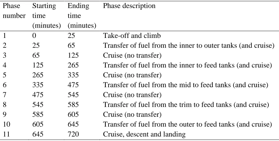
Table 2 Timings of the phased mission

Phase number

Starting time (minutes)

Ending time (minutes)

Phase description

1 0 25 Take-off and climb

2 25 65 Transfer of fuel from the inner to outer tanks (and cruise)

3 65 125 Cruise (no transfer)

4 125 265 Transfer of fuel from the inner to feed tanks (and cruise)

5 265 335 Cruise (no transfer)

6 335 475 Transfer of fuel from the mid to feed tanks (and cruise)

7 475 545 Cruise (no transfer)

8 545 585 Transfer of fuel from the trim to feed tanks (and cruise)

9 585 605 Cruise (no transfer)

10 605 645 Transfer of fuel from the outer to feed tanks (and cruise)

11 645 720 Cruise, descent and landing

It is stated in [9] that in order to prevent wing bending very little fuel is stored in the outer tanks during take-off. Therefore, immediately after take-off and climb, some of the fuel from the inner tanks is transferred to the outer tanks. All the other fuel transfer occurs when the engine feed tanks are depleted to approximately 30%. Note, it is assumed that all tanks are not run dry, and therefore, at the end of each corresponding transfer phase, there is a small quantity of fuel remaining in the tanks. The quantities of fuel in the tanks at the beginning of the mission are presented in Table 3.

Table 3 Fuel quantities at the start of the mission

Outer tank (kg)

Feed tank (kg)

Mid tank (kg)

Inner tank (kg)

Trim tank (kg)

Total (kg)

600 19000 27000 34300 15400 215200

A number of pumps in the system supply fuel at different rates. It is assumed that the supply to each of the engines is 1 kg/s [9] and 4 kg/s in cruise and take-off respectively. The transfer pumps are assumed to transfer the fuel between tanks at a rate of 3 kg/s. Note, there are a number of redundant components, including engine feed pumps, which would only be activated if the primary pump has failed, i.e. the secondary pumps will be turned on when the corresponding primary pump is diagnosed to have failed.

Each of the 62 considered components can fail at multiple points during the mission. These failure times are assumed to be in the middle of each phase, and the effects of the failure on the system are assumed to have stabilised by the next time step of the mission. Each component can fail in multiple failure states: the pumps in 7 different states and the valves in 3 failure states. For example, the pumps can fail supplying the maximum rate (i.e. 4 kg/s), the fuel transfer rate (i.e. 3 kg/s), the cruise rate (i.e. 1 kg/s), and be failed off (i.e. 0 kg/s), and can fail supplying half of each of the rates, in order to represent degraded pumps (i.e. 2 kg/s, 1.5 kg/s and 0.5 kg/s, respectively). The valves can fail fully open, fail half-open (i.e. the radius of the opening is half of the fully open valve), and fail closed.

time results in 2926 different cases of failures to consider. Of these 2926 failures, 2148 can be detected, i.e. 778 failures are hidden failures as they produce no observable symptoms. In addition, 1260 of the 2926 failures result in system failure, i.e. when the mission cannot be completed successfully, which is assumed to occur in three ways. The first of the ways that system failure can be caused is when the supply of fuel to the engines fall below 75% of the nominal amount supplied to them. The second way is when the quantity of fuel in one of the wings is significantly more than the quantity of fuel in the other wing, resulting in an imbalance of the aircraft, potentially preventing it from remaining airborne. In this paper, the threshold is set at one wing being 20% heavier than the other, but in reality this threshold would be lower. The final system failure mode is when the weight of the aircraft exceeds the maximum landing weight, with the maximum amount of remaining fuel on landing assumed to be 30000 kg, at the end of the mission due to the quantity of fuel remaining in the tanks. Note, that effects of component failures depend on the phase, as discussed in the introduction, i.e. if a transfer pump in one of the inner tanks fails off in the first phase of the mission, a large quantity of fuel would be trapped in the tank and the mission could not be completed. However, if the same transfer pump was to fail off in the fifth or later phase, when that pump is not used anymore in the mission, it will have no effect on the completion of the mission. Minimal cut sets were not obtained as a part of this study, 1260 failures that cause system failure were identified by modelling the system using if-then-else statements, discussed in section 4.1. Note that a minimal cut set, obtained from a fault tree, is a minimum combination of component failures such that if they all occur, system failure also occurs [11]. In the next section, the proposed performance metric is presented.

3. Proposed sensor performance metric

The proposed performance metric,I{s}, presented in Equation 1, is an average value of three terms: a term that considers the percentage of failures the sensors can detect,DE{s}, a term that considers the ease of diagnosis of the detected failures, DI{s}, and a term that considers the effect that the detected failures have on the successful completion of the mission,CR{s}.

The performance metric is between values of 0 and 1, where 1 is the best possible sensor, i.e. detects all the failures (including critical failures) as soon as they occur, and all component failures can be diagnosed correctly with 100% confidence. It is assumed that the failure rate,

λ, is 0.000001 and 0.000005 per time step for the pumps and the valves, respectively. This corresponds to approximately 694 and 139 days of constant use for pumps and valves, respectively. Note that the chosen values of failure rates do not affect the outcomes of the method; it only matters that the ratio between the component failure rates is realistic. Alternatively, generic component failure data could be obtained from reliability data handbooks [12]. Also note that the notation of sensorscan refer to an individual sensor or a group of sensors.

3.1. Detection term

The detection term in [1] of the performance metric considers the percentage of component failures that can be detected by the sensors. In order to detect the component failures, the sensor reading must deviate from the sensor reading that is produced in normal operating behaviour. The detection term introduced in [1] is given in Equation 2.

I{s}=

ܦܧ{௦}+ܦܫ{௦}+CR{s}

Here Pd is the sum of probabilities of considered failures’ occurrence that sensor s can detect, and Pmd is the sum of probabilities of considered failures’ occurrence that can be detected by at least one sensor out of all possible sensors on the system, i.e. in this example, there are 2148 of the 2926 considered failures that can be detected since 778 failures are hidden. The time-dependent factor considers the time of failure occurrence and the time of detection, and is shown in Equation 3. Note, the time of detection can be the same as the time of occurrence, or at any point later in the mission, even in later phases. If the mission is of length

T,and the failure occurs at timetf, then the time of detection,td, can be any value fromtftoT. HereNd{s}is the number of component failures that can be detected by the considered sensor

sand the sum ofPe overNd{s} is equal toPd., where Peis the probability of occurrence of a considered failure.

The two factors in brackets consider the delay in the detection of the failure in relation to the total length of the mission, and in relation the remaining time of the mission, respectively. The first factor does not consider when the failure occurs, only how long it takes for the failure to be detected, i.e. a 5 minute delay in a short mission will have a greater effect than a 5 minute delay in a longer mission. The second factor takes into account when in the mission the failure occurs, i.e. a failure occurring near the start of the mission influences the mission for longer than a failure occurring towards the end of the mission, and therefore, affects the detection term more. For both factors, the longer the delay between failure and detection, the smaller the factor, i.e. the less favourable the sensor combination will be. This is because it will delay any action being taken to prevent system failure, if system failure is possible to prevent. DE{s} is equal to 1 when sensorscan detect all the considered failures that are possible to detect as soon as they occur, and is equal to 0 when sensors cannot detect any of the failures that can occur on the system, i.e.Nd{s}is equal to 0.

3.2. Diagnostic term

The diagnostic term of the performance metric considers how easily a failure can be diagnosed using sensors. In order to diagnose the failures, the symptoms of different failures need to be different in order to be able to distinguish between them. The larger the number of different sensor readings,nrs, the higher the probability of diagnosing the component failures correctly, i.e. if a different sensor reading is produced for every possible component failure, all failures are diagnosed correctly. Assume each sensor reading i of sensor s will have a probability of occurrence, Psri, and one of the component failures that can cause the sensor reading will be the most likely to have caused it, where the probability of occurrence of this failure is denoted as Pmli. The higher the ratio between Pmliand Psrithe more likely that the component failure is to be diagnosed correctly. These two terms are summed over the number of sensor readings for sensors, and their ratio is denoted as the diagnostic term, presented in Equation 4.

DE{s}=

Pd

Pmd

(2)

DE{s}=

1

Pmd ෍ ܲ௘ቆ1−

൫ݐௗ − ݐ௙൯

ܶ ቇቆ1−

൫ݐௗ− ݐ௙൯

൫ܶ − ݐ௙൯ቇ ேௗ{௦}

଴

DI{s} =

∑nrsi=1Pmli ∑nrsi=1Psri

(4)

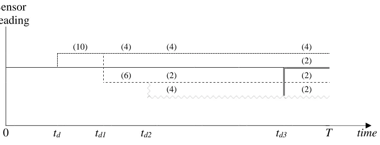
In a time-dependent case, the sensor readings may change over time after the occurrence of the failure, therefore, the diagnostic capability will also change over time. Therefore, the diagnostic term considers how soon after the detection the best diagnostic capability can be achieved, expressed as the time step at which the highest probability of correct diagnosis is achieved. In some cases, there may be a long delay between the occurrence of the failure and this time step, but a reasonably high diagnostic capability can be obtained after a significantly shorter time. Therefore, the diagnostic term considers the balance between the diagnostic capability and the time taken to achieve it. A simple example is presented in Figure 2.

Sensor reading

(10) (4) (4) (4)

(2)

(6) (2) (2)

(4) (2)

0 td td1 td2 td3 T time

Figure 2 Representation of the timeline of the mission for the diagnostic term

Note that Figure 2 presents all possible sensor outputs over time due to failures, i.e. in reality as only one sensor reading would be observed at any one time, the figure with multiple readings is only used for illustration of the diagnostics term. The solid line represents the sensor reading produced under normal operating conditions, i.e. if no failures are present (or detected) in the system. At time td, the sensor detects a failure when a different sensor reading is produced, which is represented by the dotted line, for example, a cross-feed valve is open erroneously and the flow increases. There may be a number of different component failures that are detected at this time, in this example there are 10, since they all produce the same sensor reading. At timetd1, due to changes in operation, such as the transition to a different mission phase, the sensor reading for some of the failures may deviate again. In this example, 6 of the 10 component failures produce a different sensor reading, represented by the dashed line. Therefore, if diagnostics is carried out aftertdbut beforetd1, the result will be quite poor, as 10 component failures will be diagnosed as failed; whereas if diagnostics is carried out after

td1 (and before td2), the result will be better, as a smaller number of failures (4 if the sensor reading was expressed as the dotted line, and 6 – as the dashed line) will be diagnosed as failed. This is repeated a number of times, with at timetd2the sensor reading represented by the dashed line splitting into two sensor readings, 2 of the 6 component failures producing the sensor reading represented by the dashed line, and 4 of the 6 component failures being represented by the zig-zag line. The same is the case at timetd3 with the double line. Also note that in this paper due to operational changes or failures, sensor readings change instantly; in reality there would be a gradual change from one reading to another.

For this example of 10 component failures, if no time dependence factor is considered, then

then it might be useful to have a lower diagnostic capability, but after a significantly shorter time. A factor is used to consider the effect of the time to achieve improvements in the diagnostic term. This factor is calculated for each time step, Tstep, between td and T, and is presented in Equation 5.

Similarly to the detection term factor, the two members of the equation consider the amount of time taken to achieve the best diagnostic capability of the failure in relation to the total length of the mission, and the remaining time of the mission, respectively. For each time step, the factor is calculated and multiplied by intermediate values of the diagnostic term for that considered deviated sensor reading. This results inValue(Tstep), which is presented in Equation 6. Note,ݔmaxis the number of sensor readings at each point in the mission, i.e. in the example in Figure 2,ݔmax(td) = 1,ݔmax(td1) = 2,ݔmax(td2) = 3, etc.

For simplicity, denoteN(Tstep) = ∑௫_௫ୀଵ೘ ೌೣ൫்ೞ೟೐೛൯ܲ_{௠ ௟௫}, andD(Tstep) =∑௫_௫ୀଵ೘ ೌೣ൫்ೞ೟೐೛൯ܲ_௦௥௫. The time step that results in the maximum value of the termValue(Tstep) is denoted asTstepmax, and is used in the calculation of the time-dependent diagnostic term, which is presented in Equation 7. At each time step, there can be many different deviations, observed by the sensors, therefore, the number of deviations at each time step is represented bynrs(td). This process is summed over all time steps from the earliest detection time observed,tdmin, to the end of the mission, as there are many different times at which the failure can be detected.

The diagnostic term will be equal to 1 when all component failures produce different sensor readings as soon as they occur, and will be close to 0 when many different component failures produce the same sensor reading.

3.3. Criticality term

The criticality term of the performance metric considers the effects of component failures on system performance that can be detected by sensors. This term is based on the Fussell-Vesely importance measure [13] which in this study is adapted for considering sensors. According to definition, this importance measure considers the contribution of individual components to the system unavailability, and is calculated by subtracting the probability of system failure when the considered component is working from the probability of system failure Qsys, and normalising it by the probability of system failure Qsys. The importance measure is adapted here such that the subtracted term is the probability of system failure given that the non-deviated sensor reading of sensorsoccurs,Qsys(qs= 0). The proposed criticality term is presented in Equation 8.

ܨܽܿݐ݋ݎ൫ܶ௦௧௘௣൯= ቆ1 − ൫ܶ௦௧௘௣_ܶ− ݐௗ൯ቇቆ1− ൫ܶ₍௦௧௘௣_{ܶ − ݐ}− ݐௗ൯ ௗ) ቇ

(5)

ܸ݈ܽݑ݁൫ܶ௦௧௘௣൯=

ቀ∑௫_௫ୀଵ೘ ೌೣ൫்ೞ೟೐೛൯ܲ௠ ௟௫ቁ×ܨܽܿݐ݋ݎ൫ܶ௦௧௘௣൯

∑௫௫ୀଵ೘ ೌೣ൫்ೞ೟೐೛൯ܲ௦௥௫

= ܰ(ܶ௦௧௘௣) ×_ܦ(ܨܽܿݐ݋ݎ൫ܶ_ܶ ௦௧௘௣൯

௦௧௘௣)

(6)

ܦܫ{௦} = ෍ ∑ ܰ(ܶ௦௧௘௣௠ ௔௫)௜×ܨܽܿݐ݋ݎ(ܶ௦௧௘௣௠ ௔௫)௜

௡௥௦(௧)

௜ୀଵ

∑௡௥௦௜ୀଵ(௧)ܦ(ܶ௦௧௘௣௠ ௔௫)௜ ௧ୀ்

௧ୀ௧೏೘ ೔೙

CR_{௦} =

Q_sys−Q_sys(q_௦= 0)

Q_sys (8)

As for the two previous terms, the criticality term of the time-dependent performance metric considers the amount of time between the occurrence of the failure and system failure. The time at which the system becomes critical, tc, can be any time between the time of failure,tf, and the end of the mission, T. Note, that system failure may not occur. For this term, the sooner after the occurrence of the failure that the system becomes critical, the larger the effect of the failure on the criticality term.

The amount of time that the component is in a critical state in relation to the total mission time, and the remaining mission time after the occurrence of the failure are considered. For the criticality term, the time-dependence factor is introduced to the individual terms of the criticality term, i.e. there are time-dependent expressions ofܳ_௦௬௦andܳ_௦௬௦(ݍ= 0), presented in Equations 9 and 10, respectively. Note, the summation in Equation 9 is over all critical events, Nc{s}, i.e. events that cause system failure, and this value is the same for any sensors, and the summation in Equation 10 is over all critical events that are not detected by the selected sensor,Ncnd{s}, i.e. this value is different for each sensor.

However, there is one exception to Equations 9 and 10. The system will be critical when the aircraft lands if the weight in the aircraft is above the maximum landing weight. As the aircraft cannot gain weight through the mission, if it is above the maximum landing weight at the end of the mission, it is above the maximum landing weight for the whole mission. In this sense, the system is in this critical state throughout the whole mission and the time-dependence factor is not considered, i.e. Equations 9 and 10 take account of the termPeonly.

3.4. Discussion

It is proposed that the performance metric is the average of the three terms. However, as discussed by Reeves et al. [1], there may be some applications where it is desirable to favour one term of the performance metric over the others. Therefore, the performance metric can be used to determine a number of highly ranked combinations of sensors, and then use the values of the individual terms for the final selection of the most suitable combination of sensors for a specific application. For example, the criticality term could be favoured for safety-critical systems, such as aircraft engine control systems, when early detection of critical component failures enables the mitigation of failure effects, such as emergency rerouting and landing. The diagnostic term could be favoured in situations when system down-time is expensive, such as disruptions on oil and gas rigs, and the repair work has to be completed as quickly as possible. Therefore, finding the exact component that needs maintenance can bring the system to the working state as soon as possible, and also decrease workforce exposure to a related hazard.

In order to be able to apply the performance metric to a system operating in a phased mission, the factor of time dependence is introduced. The three terms have similar factors

ܳ௦௬௦= ෍ ܲ௘ቆ1− ൫ݐ௖− ݐ_ܶ ௙൯ቇቆ1− ൫ݐ_{(ܶ − ݐ}௖− ݐ௙൯ ௙)ቇ ே೎{ೞ}

଴

(9)

ܳ௦௬௦(ݍ= 0) = ෍ ܲ௘ቆ1− ൫ݐ௖− ݐ_ܶ ௙൯ቇቆ1− ൫ݐ_{(ܶ − ݐ}௖− ݐ௙൯ ௙)ቇ ே೎೙೏{ೞ}

଴

included that consider how long the failure is present before the considered factor is achieved (detection, diagnosis or becoming critical), in comparison to the length of the mission, and the time remaining in the mission after failure occurrence, (or failure detection in the case of the diagnostics term). However, whilst all three terms require additional computational resources in comparison to the time-independent performance metric terms, the diagnostic term is significantly more computationally intensive than the other two terms. This is because the diagnostic term needs to be calculated for every remaining time step of the mission (as it may improve throughout the mission), whereas the other two terms only need to be calculated once. For example, if a failure occurs withXremaining time steps of the mission, Equations 5 and 6 for the diagnostic term need to be calculated X times, and finally the diagnostic term (the summed term of Equation 7) can be obtained. The earlier in the mission the failure occurs and the longer the mission is, the more calculations for the diagnostic term are required, whereas during the calculation of the detection and criticality terms the relevant equations are applied only once, regardless of the length of the mission or the time of failure occurrence. Therefore, for comparison, calculation of detection and criticality terms takes seconds, whereas calculation of a diagnostic terms can take several minutes.

In addition to this feature needing to be considered in the application of the method to a complex system, the determination of the most suitable sensor combination can also be time consuming, as there are a large number of different combinations of sensors to calculate the performance metric for. Therefore, in order to determine the most suitable sensor combination more efficiently, a Genetic Algorithm based optimisation process is proposed in this study, detailed in section 4.2.

4. Application of the methodology to the fuel system of the Airbus

A380-800

The proposed methodology is applied to the fuel system presented in section 2. 4.1. System modelling

The system modelling technique uses a series of if-then-else statements in a C++ script in order to determine the flow of fuel in each section of the system at each time step of the mission, by asking questions, such as, is a required pump on, is there fuel coming into a section, can fuel leave the system, etc. Input parameters are details of the mission, such as its duration and phase description, fuel levels in each tank, fuel supply rate of each pump, if the valves are open or not, component failure information, such as the probability of occurrence and its time of occurrence in a simulation, as described in section 2. This information is read from the text file into the C++ script, and the outputs, such as sensor readings, fuel levels and the state of the system (in terms of its failure mode), are obtained for every failure scenario at every time step over the duration of the mission.

4.2. Sensor selection using the GA method

As mentioned in section 2, there are a large number of hidden failures (778), i.e. failures that do not produce any observable symptoms for any of the sensors. Therefore, approximately 62% of the failures can be detected, calculated as the sum of the probability of failure occurrence for all failures that can be detected divided by the sum of the probability of failure occurrence for all failures.

less than 1 because of the time-dependence aspect, i.e. all the failures can be detected, but some of the failures are detected with some delay, i.e. the symptoms are observed later in the mission. The diagnostic term is also less than 1 because not all of the detected component failures can be diagnosed correctly, as some sensor readings are being produced by more than one component failure. Note, all critical failures can be detected as soon as, or even before, the system becomes critical, therefore, the criticality term is 1.

As it would be impractical to select all of the sensors on the system, their combinations are considered. Since there is a large number of sensors, there is also a large number of combinations of sensors to consider. For example, there are over 61 million combinations of 5 sensors and over 1.1×1013 _{combinations of 10 sensors. It is, therefore, not feasible to}

exhaustively calculate the performance metric for all the combinations of sensors, and a two-level Genetic Algorithm (GA) approach is proposed for this purpose.

Genetic algorithms were initially developed by Holland [14] and they are based on the principal of natural selection. The GA method begins by analysing a population of randomly generated strings which represent potential solutions to the problem in question [15]. Genetic operators, such as crossover, elitism and mutation, represent natural selection, and they form heuristic rules that guide the search of a solution, avoiding the evaluation of the parts of the design space where the fitness function value is low, i.e. without having to evaluate the suitability of every possible solution exhaustively. The two-level GA method, proposed in this paper, and the results are presented next.

The sensors in the GA are represented in the form of a chromosome with 96 genes, i.e. one gene for each sensor, where 1 represents that a sensor is selected, and a 0 represents that a sensor is not included. For example, for a system with 10 sensors the string, 0100010010, represents sensors 2, 6 and 9 being selected. In the proposed GA approach the fitness function is derived using the performance metric, and a constraint is introduced on the number of sensors, such that any combination of sensors that violates this constraint has a penalty factor applied, which is equal to the square of the number of sensors in the combination, as one of the types of penalty factors, suggested by Goldberg [15]. As discussed in section 3.4, the diagnostic term is significantly more computationally intensive than the other two terms, therefore, in the first level of the GA method a simplified formula of the performance metric is used as the fitness function, i.e. only the average of the detection and criticality terms. The full performance metric, as shown in Equation 1, is then used as the fitness function in the second level of the GA method.

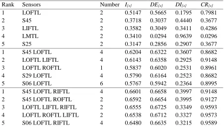
Table 4 Groups of one, two and three sensors using the exhaustive method

Rank Sensors Number I{s} DE{s} DI{s} CR{s}

1 LOFTL 2 0.5147 0.5665 0.1795 0.7981

2 S45 2 0.3718 0.3037 0.4440 0.3677

3 LIFTL 2 0.3582 0.3049 0.3411 0.4286

4 LMTL 2 0.3410 0.0294 0.9639 0.0296

5 S25 2 0.3147 0.2856 0.2907 0.3677

1 S45 LOFTL 4 0.6204 0.6322 0.3607 0.8682

2 LOFTL LIFTL 4 0.6143 0.6358 0.2925 0.9148

3 LOFTL ROFTL 1 0.5837 0.6020 0.2531 0.8961

4 S29 LOFTL 4 0.5790 0.6164 0.2523 0.8682

5 S06 LOFTL 6 0.5767 0.5942 0.2364 0.8995

1 S45 LOFTL RIFTL 4 0.6601 0.6658 0.3997 0.9148

2 S45 LOFTL ROFTL 2 0.6592 0.6654 0.3995 0.9127

3 LOFTL LIFTL RIFTL 2 0.6555 0.6725 0.3349 0.9593

4 LOFTL ROFTL LIFTL 2 0.6538 0.6712 0.3327 0.9573

5 S06 LOFTL RIFTL 4 0.6480 0.6635 0.3215 0.9589

In general, most of the individual sensors that were ranked highly are included in the combinations of two and three sensors, and the performance metric increases with each additional sensor. All of the terms in the performance metric decrease when the rank decreases, with some exceptions, for example, the combination of one sensor ranked 4th, {LMTL}, has a high diagnostic term but the detection and criticality terms are significantly lower than the ones of similarly ranked sensors. Since this sensor detects fewer component failures, it is easier to diagnose them, resulting in a higher diagnostic term, therefore, it is important to study not only the overall performance metric but also its individual terms in order to select sensors appropriately, as also discussed in section 3.4.

Table 5 presents the best solutions for each set number of sensors, denoted as column “No. S.”, when the first level of the GA method is implemented. The earliest generation in which the best solution is first achieved (out of 100) in any of the populations is given in column “Generation”, the number of populations in which the best solution is obtained given in “No. Pop.”, and the number of different combinations of sensors with the corresponding fitness value – in “No. Comb.” (both out of 50).

Table 5 Best combinations of sensors at the end of the first level of the GA method

No. S.

Sensors Fit DE{s} CR{s} Generation No.

Pop.

No. Comb.

3 S21 LOFTL RIFTL 0.8265 0.7382 0.9148 2 50 25

4 S31 ROFTL LIFTL RIFTL

0.8671 0.7749 0.9593 10 35 13

6 S10 S51 LOFTL ROFTL LIFTL RIFTL

0.9305 0.8609 1.0000 23 10 9

8 S08 S13 S21 S34 S60 S76 LOFTL RIFTL

10 S03 S08 S10 S24 S57 S65 S72 S76 ROFTL RIFTL

0.9610 0.9219 1.0000 13 46 46

12 S03 S13 S18 S22 S35 S38 S46 S72 S76 S85 ROFTLC LIFTLC

0.9610 0.9219 1.0000 8 50 50

The combinations of sensors detailed in Table 5 shows an increase in the detection and criticality terms as the number of sensors increases. It also demonstrates that the maximum value of each of the two terms can be achieved using 10 sensors and 6 sensors, respectively.

As the performance metric was calculated exhaustively for all combinations of 3 sensors, the ranking of each combination determined at this level of the GA method can be determined. The combination of 3 sensors in Table 5 is ranked 20thand there are 94 combinations of sensors with a higher performance metric than this. This is because of the diagnostic term for this combination (0.2785) is lower than other combinations, resulting in other combinations having a higher performance metric. The second level of the GA method is applied for each number of sensors (No. S.) as in the first level, and is presented in Table 6. Note, generation 0 refers to the population at the start of the second level of the GA method, i.e. before any genetic operators are applied in the second level.

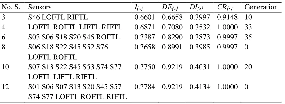
Table 6 Best combinations of sensors at the end of the second level of the GA method

No. S. Sensors I{s} DE{s} DI{s} CR{s} Generation

3 S46 LOFTL RIFTL 0.6601 0.6658 0.3997 0.9148 10

4 LOFTL ROFTL LIFTL RIFTL 0.6871 0.7080 0.3532 1.0000 33 6 S03 S06 S18 S20 S45 ROFTL 0.7387 0.8290 0.3873 0.9997 35 8 S06 S18 S22 S45 S52 S76

LOFTL ROFTL

0.7658 0.8991 0.3985 0.9997 0 10 S07 S13 S22 S45 S53 S74 S77

LOFTL LIFTL RIFTL

0.7750 0.9219 0.4031 1.0000 20 12 S01 S06 S07 S13 S20 S45 S57

S74 S77 LOFTL ROFTL RIFTL

0.7784 0.9219 0.4134 1.0000 0

The combination of three sensors in Table 6 is the same as the one ranked 1stin Table 4, i.e. using the exhaustive method. This is a significant improvement over the combination of sensors selected at the end of the first level of the GA method and also shows that the ultimate result in the case for three sensors has not been affected by the two-level method, i.e. when the diagnostic term was omitted in the first level. Whilst the best combination of sensors was obtained at the end of the second level of the GA method in this case, this would not always be the case. However, it is worth noting that this result was achieved in approximately one seventh of the time taken to calculate all 142880 combinations of three sensors exhaustively.

Also note that the combinations of 6 and 8 sensors in Table 6 do not have the criticality term of 1, but the combinations of 6 and 8 sensors in Table 5 do. However, the combinations of sensors in Table 6 can still detect all of the critical component failures but at a later modelling time step for some failures.

sensors is the tail of the aircraft. If this sensor combination was to be adapted, one of the sensors in the tail of the aircraft may not be included and a different sensor included elsewhere, perhaps in the fourth feed tank. However, this would require calculation of the performance metric for different combinations of sensors, and an increase in performance metric may not be easy to obtain. As the combination of 10 sensors in Table 6 is the smallest number of sensors that can detect all of the component failures, this combination of sensors is selected for use in the fault diagnostics process in the following section. The fault diagnostic process is applied in order to determine whether the selection of sensors, derived using the proposed method, is suitable.

4.3. Fault diagnostics

In order to verify that the chosen sensors are able to detect faults and diagnose failures, all of the sensor readings corresponding to each of the component failures are modelled and diagnosis of the component failures is attempted. In the fault diagnostic process a library of sensor readings for all of the component failures, and the sensor readings that are obtained from the model when a failure is modelled, are compared in order to determine which component failure has occurred. If there is more than one component failure that produce the same set of observed symptoms, each component failure will have a different probability of being that observed failure. This is equal to the probability of each failure occurrence, divided by the probability of all component failures that produce the observed symptoms, respectively, (Pmli/Psri), related to the diagnostic term of the performance metric.

Table 7 Diagnostic results of component failures

Diagnostic result EF pumps

FT pumps

D pumps EF valves

DR valves

CF valves

100% 262 45 - 22 52

-50% 240 15 - - 16

-a% - 100% 4 197 - - 36

-a% - 50% - 40 - - 2 10

a% - b% - 100% - 124 - - 3

-a% - b% - 50% - 20 - - -

-a% - b% - c% - 100% - 21 - - 1

-50% < a% < 100% - - - 22 -

-0% < a% < 5-0% - 72 264 - 48 48

a% - <50% - - - - 116 40

100%d 4 6 - - 55

-50%d - - - - 14 10

a% - < 100%d - 2 - - 33

-0% < a% < 5-0%d - 42 - - 216

-a% - < 50%d - - - - 24

-16.66% 22 - - - -

-0% 84 32 44 88 473 57

TOTAL 616 616 308 132 1089 165

the correct component failure will be diagnosed. Note, there are other component failures that will not be diagnosed correctly initially, but at a later point in the mission, the component failures are all diagnosed correctly.

It is worth noting that most of the hidden failures observed in the system are failures of components in the sections of the system that are not normally used, i.e. the dump and refuel valves. However, there are some hidden failures in the sections of the system that are normally used. The hidden failures of the engine feed pumps occur when the pumps fail in the states they are in during operating conditions. For example, the primary pumps failing supplying the quantity of fuel supplied in the cruise state, and the secondary pumps failing in the off state. For the transfer pumps the hidden failures are the pumps failing off after they have already transferred the fuel out of the corresponding tank.

In the next section, the analysis of the proposed methodology is given.

5. Discussion

The model of the system enables the determination of the sensor readings for all of the time steps during all of the missions. It takes less than a minute to determine the sensor readings for each of the 96 sensors, for all 720 time steps of each of the 2926 missions considered, which is negligible in comparison to the time taken to calculate the sensor performance metric.

For simpler systems, the sensor readings produced by the model could be verified manually, or by comparing to the outputs using a Bayesian Belief Network model of the system. However, as this system is complex and there are a large number of different sensor readings considered, these solutions are impractical. Therefore, a number of consistency checks were introduced in the C++ script for verification of the model. During these checks expected sensor readings for the different component states were compared with the sensor readings obtained from the model. For example, if two sensor readings used to define the presence of fuel in a section contradict each other, the modelling rules that describe fuel in this section are revised. Overall, there were 233 consistency checks included in the script, and they were tested on a large number of cases (approximately 4.2 million), which were defined by introducing all the combinations of failures of two components, occurring at different times during the mission.

The application of the two-level GA method determines suitable combinations of sensors for the fuel system. As discussed in section 4.2, there is no difference between the best combination of 3 sensors calculated exhaustively and the best combination of 3 sensors calculated using the two-level GA method. As it is not possible to determine whether the combination of 10 sensors is actually the best that can be achieved without exhaustively calculating the performance metric for all combinations of sensors, it is not possible to say how close to the best value this combination of 10 sensors is. However, this sensor combination detects all of the combinations of failures that are possible to detect, and therefore, all the critical failures. The combination of sensors diagnoses all of the component failures that can be detected successfully, apart from 22 failures. These 22 component failures can still be diagnosed correctly, if the incorrectly diagnosed components are inspected, and the evidence about their state is introduced to the model and the diagnostics are repeated. Also, the time taken to apply the two-level GA method is significantly less than the calculation of the performance metric for all combinations of sensors exhaustively.

6. Conclusions and future work

failures that can cause system failure, and favours sensors that can detect components with a higher probability of failure occurrence.

The sensor selection methodology is applied to the fuel system of the Airbus A380-800, a complex system consisting of over 60 components. The system is modelled using a C++ script to enable the automatic determination of the performance metric. To do this, a mission is considered that has several operational phases and many potential component failures. The most suitable combination of sensors is determined using a two-level GA method. This results in the determination of a suitable combination of sensors being achieved efficiently, enabling the performance metric to be calculated for combinations of up to 12 sensors. Future work could include a single-level GA method considering the full performance metric as the fitness function and comparing the results between the two methods, which would help to determine the impact of ignoring the diagnostic term on the sensor selection in the two-level GA method. Note that the execution time for the single-level GA method would be higher.

The system model accurately determines the sensor readings for all combinations of component states. It also enables the correct diagnosis of most of the detected component failures (apart from the 22 cases, discussed previously). Potential future work in this aspect could be to consider multiple component failures occurring within one mission and their effects on the resultant selection of sensors. Additionally, more component failures could be considered, for example, instead of assuming failure occurrence in the middle of the phase, failures would occur at any time in the phase, or including more failure modes, such as tank failures. The modelling time step could be reduced; due to this potentially the dynamic change (instead of instant) in sensor readings could be modelled, and the percentage of correctly diagnosed failures would increase, as deviations due to failures would be modelled to occur and, therefore, be diagnosed sooner.

Finally, the proposed method is not specific to aircraft fuel systems, i.e. the performance metric approach is suitable for other types of systems that could be modelled in terms of their sensor observations and effects of failures on system performance. The effectiveness of the selected sensor suite for fault diagnostics could be evaluated by building an extensive library of component failures and their effects on the performance of the modelled system.

7. Acknowledgements

This project is supported by BAE Systems and the Engineering and Physical Sciences Research Council (EPSRC). The authors gratefully acknowledge the support of these organisations.

References

[1] Reeves J, Remenyte-Prescott R, Andrews JD. A sensor selection method for fault diagnostics. In: Proceedings of the European Safety and Reliability Conference,Portoroz, Slovenia, 18 - 22 June 2017. 3533-3541

[2] Snooke, N., 2009. An automated failure modes and effects analysis based visual matrix approach to sensor selection and diagnosability assessment. Inonline proc. Prognostics and Health Management Conference (PHM09)

[4] Spanache, S., Escobet, T., & Travé-Massuyès, L. 2004. Sensor optimization using genetic algorithms, Proc. 15th Int. Workshop on Principles of Diag. DX, pp.179 -183

[5] Santi, L. M., Sowers, T. S., & Aguilar, R. B., 2005.Optimal sensor selection for health monitoring systems. National Aeronautics and Space Administration, Glenn Research Center.

[6] Maul, W. A., Kopasakis, G., Santi, L. M., Sowers, T. S., & Chicatelli, A., 2008.

Sensor selection and optimization for health assessment of aerospace systems.

Journal of Aerospace Computing, Information, and Communication, 5(1), 16-34

[7] Pourali, M., & Mosleh, A., 2012. A Bayesian approach to functional sensor placement optimization for system health monitoring. Prognostics and Health Management (PHM), 2012 IEEE Conference on (pp. 1-10). IEEE.

[8] Lampis, M., & Andrews, J. D., 2009.Bayesian belief networks for system fault diagnostics.Quality and Reliability Engineering International, 25(4), 409-426.

[9] Airbus, 2006. A380-800 Flight Deck and Systems Briefing for Pilots, Issue 02.AIRBUS SAS

[10] Langton, R., Clark, C., Hewitt, M., & Richards, L., 2009.Aircraft fuel systems.

First Edition, John Wiley & Sons, Ltd

[11] Andrews, J. D. & Moss T. R., 2002. Reliability and Risk Assessment. Second Edition, Professional Engineering Publishing Limited, London and Bury St. Edmunds, UK.

[12] Moss, T.R., 2004. The Reliability Data Handbook. Wiley-Balckwell.

[13] Cheok, M.C., Parry, G. W., & Sherry R. R., 1998. Use of importance measures in risk-informed regulatory applications. Reliability Engineering & System Safety, 60(3), 213-226.

[14] Holland, J. H., 1975. Adaptation in natural and artificial systems.University of Michigan Press, Ann Arbor.