A New Analysis for Finding the Optimum Power Rating of Low Voltage
Distribution Power Electronics Based on Statistics and Probabilities
Amin Ganjavi, Edward Christopher, C. Mark Johnson, Jon Clare
University of Nottingham
Department of Electrical and Electronic Engineering, University Park
Nottingham, UK, NG7 2RD
Tel: +44 (0) 115 9515151
E-mail: [email protected]
Acknowledgments
The support of EPSRC Grants EP/K035096/1, EP/K035304/1 (Underpinning Power Electronics) and EP/I031707/1 (Transformation of the Top and Tail of Energy Networks) in undertaking this work is gratefully acknowledged.
Keywords
≪Estimation technique≫, ≪Power management≫, ≪Regulation≫, ≪Simulation≫
Abstract
The continuing trend toward heavier load and high penetration of Distribution Generation (DG) units in low voltage rural distribution feeders requires power electronic-based solution alternatives for voltage regulation purposes. The design of power electronics in terms of size and cost used for feeder voltage regulation is proportional to their KVA ratings. An iterative optimisation algorithm known as Expectation Maximization (EM) is used to identify a powerful probability model known as Gaussian Mixture Model (GMM). This leads to find an optimum KVA rating based on probabilities.
Introduction
The continued growth in electrical energy consumption has affected the voltage profile in low voltage (LV) networks. Therefore, studies concerning performance of distribution systems and quality of the service in terms of power quality and satisfactory voltage level has gained more consideration. There are numerous ways to keep distribution voltages within permissible limits (230V, +10% -6% for the UK). Some of the notable voltage regulation solutions based on power electronics for LV distribution substations are Distribution Static Compensator (DSTATCOM), Dynamic Voltage Restorer (DVR), Unified Power Quality Conditioner (UPFC), Interline Power Flow Controller (IPFC) and Solid State Transformer (SST or fully electronic transformer) [1]-[3].
The size and cost of power electronics is proportional to their power rating. The power rating of converters used for feeder voltage regulation is mainly based on substation voltage and feeder current which is influenced by load models. Load models has no certain pattern or predicted behaviour due to large range of data and changes in energy consumption. Therefore; in order to find the required distribution KVA rating of power electronics under optimal conditions, a powerful analysis based on probabilistic structure is required. Several researches have been carried out to model the distribution power flow and load through different probability distributions [4]-[12].
system with yearly load profile and the optimum substation voltage and required power converter ratings based on statistics and probabilities are obtained.
Basic Configuration
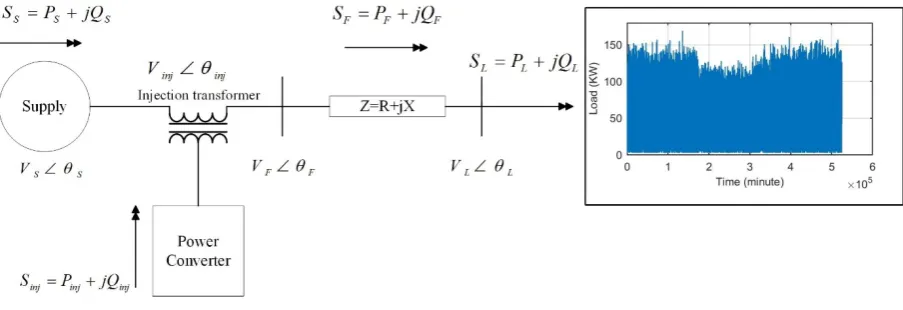
Fig.1 shows the basic configuration of the tested system. The feeder is connected to 100 residential houses by a 300m long and 300mm2 cable. The load profile is generated by CREST load model [13]
for one year (525,600 minutes). , and indicate the feeder voltage, supply voltage and injection voltage respectively.
It is assumed that the series compensator is implemented by DC-to-AC converter on feeder
(substation-end) with an energy storage device on the DC side. The aim of using power electronic is to keep the load voltage at the desired value, 230V, by injecting the lowest possible compensating voltage in series with the supply and feeder to regulate the load terminal voltage during voltage disturbances such as sag and swell.
By referring to Fig. 1. and knowing that = ∠ , = ∠ and = ∠ the power flow calculations of substation and feeder can be given by:
= + = . −
∗
(1)
= + = . −
∗
(2)
and the power flow of the series power converter can be expressed as:
= − (3)
It is preferred to have a power converter on system to be switched off most of the time to minimise the power rating, losses, size and cost of the power electronics. As a result; it is assumed that = 0
( = ); thus, by referring to equation (1), the substation power flow and voltage can be written by (4) and (5) respectively (the substation impedance is neglected):
= + (4)
[image:2.595.72.524.121.276.2]and
= + ∗ (5)
Gaussian Mixture Model and Expectation Maximization Algorithm
Gaussian Mixture Model
GMM is powerful probability model that has been widely used in fields of pattern recognition,
information processing, data mining, error correction codes, etc. GMM has the functionality to present a model representing one or several clusters with each cluster being different from one other. The data points within the same group can be properly fitted by a Gaussian distribution [14], [15]. GMM is a beneficial technique that allows different types of load distributions to be presented as a combination of several ones with their own respective means and variances.
If samples , , … , ∈ and random variable x is Gaussian, a GMM can be defined by making each i thcomponent a Gaussian density with mean, , and covariance , ∑ , as shown in equation (6):
( | ) =
(2 ) / |∑ | / (
( ) ∑ ( )=
= ( | , ∑ ) (6)
where = {( , , )} .
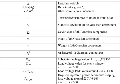
Random variable
( | ) Density of x given
∈ Observation of d-dimensional
Threshold considered as 0.001 in simulation Standard deviation of ith Gaussian component
∑ Covariance of ith Gaussian component Mean of ith Gaussian component Weight of ith Gaussian component variance of ith Gaussian component Substation voltage value k=1,…,526500 Load voltage value for every minute m=1,…,526500
Load voltage PDF value around 230V,±1%
,
Required injection power per minute keeping load voltage around 230V,±1%
[image:3.595.87.508.195.490.2]By referring to equation (6), the Probability Density Function (PDF) for a single and N Gaussian components is represented by equation (7) and (8), respectively:
( | , ) = 1 √2
( )
(7)
PDF for N Gaussian:
( | , , ) =
√2
( )
(8)
where is the weight of the i th Gaussian component and ∑ = 1.
Expectation Maximization
The challenge of estimating key parameters, such as mean and variance for a set of random data (e.g. load), that determines a mixture density, has been researched for many years. The EM algorithm is one of such complex methods. When the data is incomplete or has missing values, it helps to determine the closest estimation of the parameters of an underlying distribution from a given data set [16], [17]. EM takes observed data ‘x’ anditeratively carries out estimations to complete the data set ‘y’, which leads to then iteratively detecting that maximises ( | ) over [18]. Estimating parameters for Gaussian mixture model by using EM algorithm can be summarised in four main steps as follows:
Step 1: Initialization
The algorithm starts from some initial estimates of ( )where mth iterationhappens at the ith Gaussian
component. For example, the initial estimates of ( ), ( ), ∑( ) are chosen and for jth sample fitted to ith Gaussian component, the initial log-likelihood can be calculated by using equation (6):
( )=1 log ( ( ) ( ), ∑( ) (9)
Step 2: E-step
Computing ( ) which is the guess at the mth iteration of the probability that the jth sample belongs to
the ith Gaussian component:
( ) =
( ) ( ), ∑( )
∑ ( ) ( ), ∑( ) (10)
and
( )= ( ) , = 1, … , (11)
Step 3: M-step
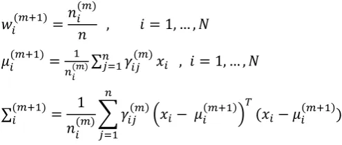
( )= ( ) , = 1, … , (12) ( )=
( )∑
( ) , = 1, … , (13)
∑( )= ( )1 ( ) − ( ) ( − ( )) (14)
Step 4: Convergence Check
By referring to equation (9) the new log-likelihood can be given by:
( ) =1 log ( ) ( ), ∑( ) (15)
If ( ) > ( ) the procedures return to step 2 otherwise the algorithm ends [18]. More details
about EM algorithm can be found in [19]-[21].
Optimum Substation Voltage Base on Yearly Load Profile
For carrying out the simulation, the yearly 100 residential load data mentioned before is used. The resolution of time scale is in minute thus, for one year the tested load profile consists of 525,600 data. It is assumed that for this load profile, substation phase voltage must have a range 230 < < 270 with = 1, … ,525600. Subsequently, for every minute of load demandin a whole year, one value of is applied and by referring to equation (5) the voltages at the load side, ( = 1, … ,526,600), are calculated. The results can be seen in Table II.
525,600 data
525,600 data 230
(V) … 239 (V) … 252 (V) … 270 (V)
(V) 226 … 221.5 … 222.8 … 216.6
. . . . . . . . . . . . . . . . . . . . . . . .
(V) 216 … 227.1 … 231.6 … 228.7
. . . . . . . . . . . . . . . . . . . . . . . .
(V) 222 … 232.8 … 246.3 … 240.8
. . . . . . . . . . . . . . . . . . . . . . . .
[image:5.595.70.318.84.189.2](V) 216 … 230 … 241 … 238.8
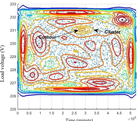
EM algorithm receives the parameters of the Gaussian distribution by creating sampling from the given set of data. Fig. 2 shows the estimated probability density cluster obtained from EM algorithm when the substation phase voltage is selected to be 239V. The scatter data points of Fig.2 represent the load voltage for every minute. As it can be seen, there is a set of load voltage data (scatter data) per cluster and each cluster represents a single Gaussian distribution containing several contours. The centre of the smallest contour of each cluster is the corresponding mixture component (peak of the Gaussian distribution curve), and the length of the largest contour of each cluster is approximately equal to 6
.
Now by having distribution parameters of each Gaussian component, the 3-dimentional and 2-dimensional load voltage probability density function (PDF) of individual Gaussians and mixture Gaussians of the substation at 239V for the whole year can be acquired and the result can be seen in Fig. 3. Each surface of Fig. 3(a) represents an overall density component compromised of several component densities (200 Gaussian distributions in total). In addition, as shown in Fig. 3(b), at selected substation voltage, 239V, load voltage has a PDF value around 230V, which for this paper is referred as PDF230.Fig. 2: Estimated probability density clusters of yearly load voltages for = 239
Fig. 3: GMM PDFs of yearly load voltages for = 239 . a) Three-dimensional GMM PDFs b) 2-dimensional GMM PDFs
a) b)
Load voltage (V) Load voltage (V)
Time (minute)
Time (minute)
Lo
ad
vo
lt
age (
V
)
`
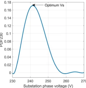
The final result of all PDF values per different substation voltages ( ) can be seen in Fig. 4. The most probable range for PDF for this type of load is 232 < < 257 with the most optimum point being at V, = 242.5 . Outside of this range, there is no probability for the load voltage to be around 230V.
Optimum Converter Power Rating
In order to assess the feasibility of the previous section, the chosen V, (242.5V) is used for the
system to determine the probability density of the converter power rating based on the tested load. By referring to equation (3) and with the assumption that feeder and converter current is equal, the power injected by the series power converter into the system for each minute is calculated and the results for 10 random substation voltages including optimum voltage (V, ) can be given in Table III. Table III shows that the selected optimum substation voltage has the lowest amount of total injected power for the whole year. Consequently, for the tested 100 residential houses, choosing = 242.5 allows the converter to operate at its lowest power rating and this produces the most efficient power electronic design with lower losses, cost, size and higher efficiency.
230V 233.7V 237.6V 242.5V
(optimum)
245.2V 249.1V 252.8V 256.6V 260.4V 270V
,(KVA) 0.1 0.25 0.35 0.67 0.88 1.2 1.47 1.6 1.9 2.6 , , (KVA) 6.1 4.6 3 1.2 1.4 1.7 3.2 4 5 6 , , (KVA) 3.1 2 0.9 0.3 1.2 2.6 3.5 4.3 5.5 8.3
[image:7.595.208.388.81.264.2](MVA) 18.2 13 8.6 5.9 6.2 9.1 14 19 24 38
[image:7.595.73.543.569.750.2]Now by referring to equations (8), the Cumulative Distribution Function (CDF) of the random variable
x can be defined in equation (16) below:
( ≤ ) = ( | , , ) = 1
√2
( )
(16)
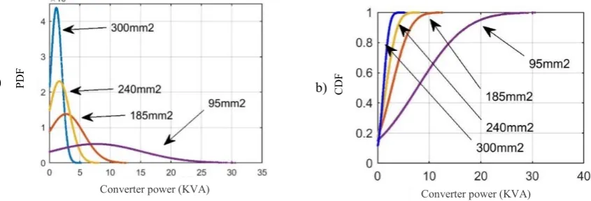
The PDF and CDF of the power converter with respect to optimum substation voltage for 100 residential houses with 300 m, 300 mm cable over a year can be found and the results are plotted in Fig. 5. It is expected to get the peak value of PDF shown in Fig. 5(a) at 0 KVA, but due to real load data variations for residential house over a year, it is impossible to obtain the highest PDF at 0KVA. Furthermore; as it can be seen in Fig. 5(b) power converter with 2.3 KVA power rating can satisfy the load voltage to be around 230V at 90% of the time, and a power converter with 3.5 KVA power rating can guarantee load voltage satisfaction 99% of the time. . In addition, 15% of the time during the whole year, the power converter does not inject any power into the system. The same procedures have been carried out for different types of cable in size and results can be shown in Fig. 6.
a) b)
Fig. 5: a) PDF of converter KVA at V, = 242.5 , b) CDF of converter KVA at
V, = 242.5 for a 300m 300mm2 cable
a) b)
Fig. 6: a) PDF of converter KVA, b) CDF of converter KVA for different cable sizes at their V, , 300m length cable
Converter power (KVA) Converter power (KVA)
Converter power (KVA) Converter power (KVA)
CD
F
CD
[image:8.595.95.511.336.490.2] [image:8.595.97.520.553.697.2]It is worth to note that the calculations are based on the assumption that load voltage is kept at approximately 230V. However; in the UK, the regulatory voltage levels are 230V, +10%-6%. In addition, some variables such as population growth, geographical factors, community development plans and substation fault, might affect the total power rating of converters. As a result, the power network planner should take the mentioned variable factors into account by increasing the total KVA rating of power converters, for instance 20% of total rating.
Conclusion
A comprehensive novel study has been carried out to evaluate probabilistic load data concerning the time-evolution of any type of load for any duration of time. Substation voltage selection plays an essential role in power system in terms of load voltage quality, network losses, power system safety, etc. A new method has been introduced to find an optimal substation voltage (V, ) for distribution system based on statistics and probabilities. This finding points to the conclusion that for a system with series set up of power converter (for voltage regulation purposes), choosing V, leads to the lowest amount of total injected power, power rating and cost of the power electronics. The explained method can be used in any probabilistic based power system analysis for any time duration including distribution planning, probabilistic load flow, load forecasting, load management, distribution automation, etc.
References
[1] S. Corsi,, Voltage control and protection in electrical power systems : from system components to wide-area control. London: Springer. pp.44-61. 2015
[2] M. Moradlou and H. R. Karshenas, "Design Strategy for Optimum Rating Selection of Interline DVR," in IEEE Transactions on Power Delivery, vol. 26, no. 1, pp. 242-249, Jan. 2011.
[3] X. She, A. Q. Huang and R. Burgos, "Review of Solid-State Transformer Technologies and Their Application in Power Distribution Systems," in IEEE Journal of Emerging and Selected Topics in Power Electronics, vol. 1, no. 3, pp. 186-198, Sept. 2013.
[4] Cagni, E. Carpaneto, G. Chicco and R. Napoli, "Characterisation of the aggregated load patterns for extraurban residential customer groups," Electrotechnical Conference, 2004. MELECON 2004. Proceedings of the 12th IEEE Mediterranean, 2004, pp. 951-954 Vol.3.
[5] C. F. Walker and J. L. Pokoski, "Residential Load Shape Modelling Based on Customer Behavior," in IEEE Transactions on Power Apparatus and Systems, vol. PAS-104, no. 7, pp. 1703-1711, July 1985.
[6] E. Carpaneto and G. Chicco, "Probabilistic characterisation of the aggregated residential load patterns," in IET Generation, Transmission & Distribution, vol. 2, no. 3, pp. 373-382, May 2008.
[7] E. Carpaneto and G. Chicco, "Probability distributions of the aggregated residential load," Probabilistic Methods Applied to Power Systems, 2006. PMAPS 2006. International Conference on, Stockholm, 2006, pp. 1-6.
[8] Seppala, "Statistical distribution of customer load profiles," Energy Management and Power Delivery, 1995. Proceedings of EMPD '95., 1995 International Conference on, 1995, pp. 696-701 vol.2.
[9] R. Singh, B. C. Pal and R. A. Jabr, "Statistical Representation of Distribution System Loads Using Gaussian Mixture Model," in IEEE Transactions on Power Systems, vol. 25, no. 1, pp. 29-37, Feb. 2010.
[10]D. H. O. McQueen, P. R. Hyland and S. J. Watson, "Monte Carlo simulation of residential electricity demand for forecasting maximum demand on distribution networks," in IEEE Transactions on Power Systems, vol. 19, no. 3, pp. 1685-1689, Aug. 2004.
[11]HERMAN R., HEUNIS S.W.: ‘Load models for mixed domestic and fixed, constant power loads for use in
probabilistic LV feeder analysis’, Electr. Power Syst. Res., 2003, 66, pp. 149– 153
[12]S. W. Heunis and R. Herman, "A probabilistic model for residential consumer loads," in IEEE Transactions on Power Systems, vol. 17, no. 3, pp. 621-625, Aug 2002.
[13]Richardson, M. Thomson, Domestic electricity demand model-simulation example, Loughborough
University, http://hdl.handle.net/2134/5786, 2010.
[15]D. F. Crouse, P. Willett, K. Pattipati and L. Svensson, "A look at Gaussian mixture reduction algorithms," Information Fusion (FUSION), 2011 Proceedings of the 14th International Conference on, Chicago, IL, 2011, pp. 1-8.
[16]J. A. Bilmes, “A gentle tutorial on the EM algorithm and its application to parameter estimation for Gaussian mixture and hidden Markov models,” Tech. Rep. TR-97-021, International Computer Science Institute, April 1998
[17]R. A. Redner and H. F. Walker, “Mixture densities, maximum likelihood and the EM algorithm,” SIAM
Review, vol. 26, pp. 195–239, April 1984.
[18]Yihua Chen, M. R. Gupta "EM demystified: An Expectation-Maximization Tutorial,". Seattle, Tech. Rep. UWEETR-2010-0002 University of Washington, Feb. 2010
[19]R. M. Neal and G. E. Hinton, “A view of the EM algorithm that justifies incremental, sparse, and other variants,” in Learning in Graphical Models (M. I. Jordan, ed.), MIT Press, Nov. 1998.
[20]L. Xu and M. I. Jordan, “On convergence properties of the EM algorithm for Gaussian mixtures,” Neural Computation, vol. 8, pp. 129–151, Jan. 1996
[21]P. Dempster, N. M. Laird, and D. B. Rubin, “Maximum likelihood from incomplete data via the EM