Accelerating Petri Net simulations using NVIDIA graphics processing units

This is an accepted manuscript of an article published by Elsevier B.V. in the European Journal of Operational Research, accepted on the 30th of June 2017, available online at: http://dx.doi.org/10.1016/j.ejor.2017.06.068.

Accelerating Petri-Net Simulations using NVIDIA Graphics Processing Units

Panayioti C. Yianni1_{, Luis C. Neves}2_{, Dovile Rama}2_{, John D. Andrews}I2

Abstract

Stochastic Petri-Nets (PNs) are combined with General-Purpose Graphics Processing Units (GPGPUs) to develop a fast and low cost framework for PN modelling. GPGPUs are composed of many smaller, parallel compute units which has made them ideally suited to highly parallelized computing tasks. Monte Carlo (MC) simulation is used to evaluate the probabilistic performance of the system. The high computational cost of this approach is mitigated through parallelisation. The efficiency of different approaches to parallelization of the problem is evaluated. The developed framework is then used on a PN model example which supports decision-making in the field of infrastructure asset management. The model incorporates deterioration, inspection and maintenance into a complete decision-support tool. The results obtained show that this method allows the combination of complex PN modelling with rapid computation in a desktop computer.

Keywords: CUDA, GPU, Monte Carlo, Petri-Net, Parallel, Asset Management, Railway

1. Introduction

Petri-Nets (PNs) have been gaining in popularity in the field of Operations Research, specifically for work-flow management systems (Salimifard and Wright, 2001), supply chains (Viswanadham and Raghavan, 2000) and enterprise resource planning (Aloini et al., 2012). One of the limitations of PNs in conjunction with probabilistic transitions is the requirement for Monte Carlo (MC) simulations resulting in high computational cost. Studies have been undertaken into accelerating PNs with General-Purpose Graphics Processing Units (GPGPUs), however these have mostly been in the fields of Biology and Physics.

The use of MC methods is very popular in science, engineering and economics research. Over time MC-based models have gotten progressively more sophisticated which often means longer computa-tion times, limiting their applicability. The use of Graphics Processing Units (GPUs) in academia as GPGPUs is gaining in popularity as it has the potential to dramatically decrease computation time allowing for much faster throughput. At the same time, the technological development of GPUs and

I_{Corresponding author: John D. Andrews; Email:[email protected]}

1_{Amey Strategic Consulting and Technology, Furnival St., London, EC4A 1AB, United Kingdom.}

2_{Resilience Engineering Research Group, University of Nottingham, Faculty of Engineering, University Park,}

their progression into general computing has meant that the cost per computing core has dropped significantly.

This study investigates the suitability of GPGPU acceleration with PNs for a decision support tool, in this case using an example from asset management. Asset management models often combine engineering, management and economics to be able to make informed decisions. A simple PN example is used as a proof of concept and then the same approach is applied to an established railway bridge model. This model was selected as it contains a number of complex PN features and therefore would be appropriate to test the suitability of GPGPU acceleration. The bridge model used as the example in this study provides predictions of condition over time, including the effects of maintenance actions and the associated costs.

Although the study uses a railway bridge asset management example, many of the topics discussed are appropriate for GPGPU acceleration of general decision support PN models. As decision support tools become more engrained into business practices and as the adoption of PNs as a modelling approach becomes more common, their efficient computation will become more important.

2. Simulation Acceleration using GPGPUs

A number of studies have been undertaken in the field of Physics to accelerate MC-based models with GPGPUs. Although not directly related to PNs, the application of the GPGPU to the modelling approach is relevant.

Tomov et al. (2005) performed a study to investigate the suitability of GPGPUs with 2D and 3D Ising models. An Ising model represents the spin of magnetism in a lattice structure. Each of the magnets can be in one of two states. The model becomes more complex when considered in a 3D space. The authors state that the common way of incorporating MC methods into the Ising model is to choose a random path through the magnets, at each magnet generating a random number which decides whether the spin should be reversed or not. At this time the Compute Unified Device Architecture (CUDA) framework (the standard framework for GPGPU development currently) was yet to be established and so an older framework known as Cg was used. The GPU used was an NVIDIA NV30, a high-end GPU from 2003. The authors conclude that the GPGPU implementation of the Ising model is three times faster than the Central Processing Unit (CPU) implementation on average. This holds true for both the 2D and 3D examples tested. The authors mention that the GPGPU performance may have been limited due to branching as the contemporary GPU used for this study did not support this feature.

Yang et al. (2007) used the power of GPGPUs to accelerate molecular dynamics. The study involved simulations to calculate thermal properties. The process of simulating molecules involves a 3D grid of interacting nodes. Simulations are carried out where the amount of energy passed from atom to atom is recorded. The stochastic nature of the modelling is due to the movement of molecules based on a decision which uses random numbers. They used an NVIDIA GeForce 7800 GTX, a high-end card from 2005. They used the Cg programming framework with 600,000 iterations per simulation. The number of atoms in the simulation was tested against the execution time. The results show that the execution time almost follows an exponential curve with the number of atoms in the simulation. In every test, the GPGPU execution is quicker than that of the CPU. The authors conclude that their average speed-up factor is between 10 and 11 times using the GPGPU.

van Meel et al. (2008) also use GPGPUs with molecular dynamics. They implement the N-squared molecular dynamics algorithm for their simulations. In contrast to Yang et al. (2007), the CUDA framework had been released by this point. They perform an interesting comparison between the simulations performed on (1) a CPU, (2) GPGPU with Cg and (3) GPGPU with CUDA. As well as the update in programming framework, they use a newer GPU from Yang et al. (2007): an NVIDIA GeForce 8800 GTX. Their results show that the GPGPU with Cg performs around 40 times faster than the CPU implementation. Using the newer CUDA framework, they manage an 80 times speed-up factor over the CPU execution.

Geist et al. (2005) was one of the first studies to try to accelerate PNs with GPGPUs. They use an NVIDIA GeForce 6800 Ultra, a high-end GPU from 2004. The authors create a PN simulator using Cg called “Cgpetri”. They compare this to serial PN simulators “xpetri” (Geist et al., 1994) and “SPNP” (Hirel et al., 2000). The example of the dining philosophers was used in the study, created by E. W. Dijkstra, but formalised by Hoare (1978). This is a common example of a PN with conflict conditions. These arise because each philosopher requires two forks to eat with, however there are too few forks to satisfy each diner. Therefore, the resource must be shared which means that the diners alternate between two condition states. They test the example ranging from 25 diners to 400 diners, recording the execution time. When there are few diners, execution on the CPU is faster as the data does not need to be packaged, passed to the GPGPU and then transferred back after computation. However, the critical point in this example is at 50 philosophers; beyond which the GPGPU based simulator outperforms the serial simulators. For example, when the number of philosophers reaches 75, the execution time of the serial simulator SPNP is approximately 38 seconds. This is almost twice as long as that of the GPGPU based simulator, which is approximately equal to 18 seconds. The serial simulators follow an almost exponential execution time with the number of diners, however when run with Cgpetri the execution time is approximately linear as a function of the number of diners.

that are created in the simulation, the more detailed the resulting outputs. There has been studies performed to parallelize Lattice-Boltzmann models and a common approach is to divide the problem into “subcubes” for concurrent computation. The authors propose a PN to schedule the computation of these subcubes to increase efficiency. Again they compare Cgpetri to xpetri and SPNP. They increase the number of places in the flow net, recording the execution time. Again, it can be seen that when the number of places in the flow net is small, the overhead of using the GPGPU means that the execution is slower. However, the advantage of the GPGPU quickly shows its strength as the execution time is almost the same across the whole range of places tested whilst the serial simulators experience significant slow down. The authors close with a comment that Moore’s Law, a characteristic applied to CPU development, means that their performance seems to double every 18 months (Schaller, 1997). However, the rate of development of GPUs is closer to doubling every 6 months. Therefore, not only was the GPGPU already accelerating the simulations but the difference was set to increase even more. Chalkidis et al. (2011) also attempt to accelerate PNs with GPGPUs. They use a real world example from the field of biology, specifically microbiology, and medicine. They claim that using a state-of-the art modelling approach, PNs in this instance, with GPGPU acceleration is the next step in producing fast, accurate, modelling results. They use the CUDA programming framework with an NVIDIA GeForce 8800, a mid-range GPU from 2006. They explain that they use Hybrid Functional PNs and detail its decomposition for GPGPU programming. They mention that the possible acceleration could be significant if they could parallelize their PN. They do so by splitting their PN into three processes hierarchically. Processes one and two are able to be simulated concurrently as they do not interact directly. Then process three can use the results of processes one and two to finish the simulation. Theoretically, by using this approach the PN simulation could experience a 1.5 times speed-up factor in serial operation. However, when considering the massively parallel characteristic of GPUs, the speed-up could be significantly higher. They conclude by saying that their average PN acceleration when using the GPGPU was 18 times faster than the serial execution.

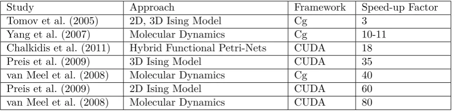
In summary, a number of studies have been undertaken accelerating simulations in the fields of Physics and Mathematics. Table 1 shows the results of the average speed-up factor in each of these studies. It can be seen that earlier implementations using Cg did not provide as much speed-up as later versions using CUDA. This occurs because: (1) the CUDA framework provided updated algorithms, processes and techniques which would help efficiency and (2) although the studies were carried out with contemporary CPUs and GPUs, the advancement of GPU compute capability outstrips the development of CPUs and so the difference in compute performance grows with time.

3. Petri-Nets

Table 1: Results of the execution time of a simple PN when computing on various devices.

Study Approach Framework Speed-up Factor

Tomov et al. (2005) 2D, 3D Ising Model Cg 3

Yang et al. (2007) Molecular Dynamics Cg 10-11

Chalkidis et al. (2011) Hybrid Functional Petri-Nets CUDA 18

Preis et al. (2009) 3D Ising Model CUDA 35

van Meel et al. (2008) Molecular Dynamics Cg 40

Preis et al. (2009) 2D Ising Model CUDA 60

van Meel et al. (2008) Molecular Dynamics CUDA 80

coloured stochastic PNs to model and evaluate workflow management in business processes. Proposed method merges control and data flow as well as organisational aspects in a single business process model. The performance of the constructed model is evaluated by discrete-event simulations. Hosseini et al. (1999) used generalised stochastic PNs to represent and analyse a hybrid maintenance model of systems with both deterioration and Poisson failures. The great modelling power of PNs allowed complex features to be easily incorporated into the model, such as pre-planned and on- condition maintenance, imperfect and sequential inspections as well as dealing with different deterioration rates at different deterioration stages. This makes the model more applicable to real world complex systems. Archetti et al. (1987) used stochastic PNs for the analysis of flexible manufacturing systems. They developed a technique for evaluating the performance of a transfer line whose stations are subject to failures, during which work pieces can be either blocked or routed to other machines. The authors computed the mean manufacturing time of work pieces in a transfer line under different control policies of a work piece using a proposed marked token technique.

PNs are constructed with two types of nodes: places and transitions. Places refer to the state of the system or an activity being undertaken in the system. Transitions cause the movement of tokens from place to place, indicating a change in the system state. Simple transitions are triggered by a time delay. No two transitions or places can be directly connected. Tokens are one of the most important components of a PN, their presence or absence in a place indicates the current system state. For example, a token occupying a place labelled “processing” could indicate that the system is in a processing activity before the next procedure. A transition, in this example, could then move the token to a place labelled “processed” when the procedure had been completed. The dependencies between places and transitions are represented by edges, connecting the places and transitions to form the net of a PN. More details can be found in Schneeweiss (2004).

understanding of the average system behaviour. This process often relies on a MC approach, hence the dependency between stochastic PNs and MC.

Additional PN features can be used in the model, if required, including multiplicity and inhibitor edges. Multiplicity is designed to modify the number of tokens required for the transition to be enabled. For example, an edge marked with “3” would mean that the transition would only be enabled when the connected place contained three or more tokens. Inhibitor edges are used to restrict firing of a transition. The presence/absence of a token in the corresponding place can either enable or disable the inhibitor edge from activation which in turn allows or disallows the transition to fire. More advanced PN features can be found in (Le and Andrews, 2016).

3.1. Example Algorithm for Petri-Net Simulation

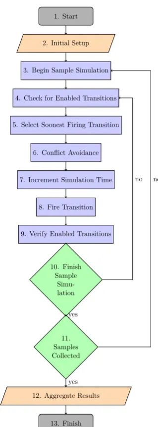
An example algorithm for PN simulation can be seen in Figure 1, represented by a flow diagram. The initial set-up of the PN is represented as an input node as often there will be some processing of data to construct the PN. Then the number of samples required will be represented by a loop. Within each of the samples there will be a further loop. This process starts with the checking of the transitions to see which are enabled (stage 4 in Figure 1). This can be quite a computationally expensive process as every transition needs to be checked to see if all its input places are marked (contain at least one token) and there are no active inhibitors on the transition (Jensen and Kristensen, 2009). The transitions which are enabled can then generate a transition firing time; stochastic transitions would call random numbers at this stage. Conflicts (i.e. two transitions are due to fire at the same time using the same input tokens) must be avoided (stage 6 in Figure 1). Two transitions with the same transition time that do not interfere with each other can fire simultaneously. The enabled transition(s) with the shortest transition time would be selected for firing. The simulation time is then increased to the point of the next transition firing. Upon firing, the input tokens are removed from the places. New tokens are generated in the output places (Andrews, 2013). Stage 9 in the figure represents a post-firing check which is to remove any transitions which were marked as enabled but are no longer enabled as the token has moved from the input place. The simulation time is checked to see whether the required simulated period has finished (e.g. 50 years). If not, the process restarts from stage 4. When the simulation time has elapsed, the sample is complete. Stage 11 checks whether the required number of samples has been run. Stage 12 aggregates the results as an output node as often the results will be analysed afterwards. Finally, the algorithm terminates.

3.2. Pleasingly Parallel Algorithms

1. Start

2. Initial Setup

3. Begin Sample Simulation

4. Check for Enabled Transitions

5. Select Soonest Firing Transition

6. Conflict Avoidance

7. Increment Simulation Time

8. Fire Transition

9. Verify Enabled Transitions

10. Finish Sample

Simu-lation

11. Samples Collected

12. Aggregate Results

13. Finish yes

no

yes

no

Figure 1: Flowchart of a stochastic Petri-Net (PN).

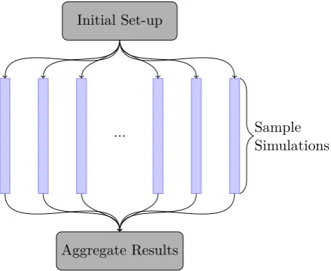
There are a number of different ways to parallelize PNs. Chalkidis et al. (2011) demonstrated a PN which could be split up for the purposes of parallelization. The overall PN was split up into three sections. The two independent sections of the PN were simulated in parallel to reduce compute times. Then the third was able to aggregate the outcome of the two independent sections to simulate the overall model outcome. The advantage of this method is that it promotes hierarchical PNs where a number of sub-nets can be simulated in parallel. The nets further up the hierarchy are then able to continue with the simulation aggregating the outcome of their subordinate sub-nets.

section labelled “Sample Simulations” could include Stages 4 to 10 of the PN algorithm in Figure 1.

Initial Set-up

Aggregate Results

... Sample

Simulations

Figure 2: A schematic demonstrating how a group of MC samples can be executed in parallel.

4. Processing Units

4.1. Central Processing Units (CPUs)

All computers contain a CPU which could be considered the centre of compute functionality. Tradi-tionally, the CPU only contained one core on which to perform calculations. More recently, multi-core CPUs have become available which are able to perform multiple calculations simultaneously. Due to industry technologies, however, a dual-core system may be able to perform more than two calculations in an instance. For this reason compute capabilities of a processing unit are compared in terms of the number of “threads” which the processor is able to utilise at any given moment. For example, a modern CPU may have four cores which could support up to eight threads.

A typical schematic of a CPU is shown in Figure 3. The CPU contains some fast temporary storage as well as some control circuitry. These all serve to provide the cores with the data they require, maximising throughput. The example CPU in the figure contains four cores which is typical of a modern CPU.

4.2. Graphics Processing Units (GPUs)

Control

Cache

DRAM

Core Core

Core Core

Figure 3: A schematic of a typical CPU, recreated from NVIDIA Corporation (2015).

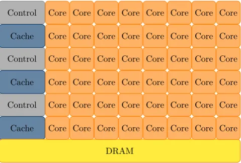
and apply a function to it. The more pixels that could be processed at once, the faster the production of the overall frame would be. Hence, the evolution of the GPU as a massively parallel processing unit. In comparison to CPUs, a GPU may have many more cores, but each individual core is slower. A schematic of a GPU can be seen in Figure 4. It can be seen that there are many more cores than the CPU seen in Figure 3. Additionally, rather than the whole processing unit sharing the cache and control units, there are multiple cache and control units. This is because GPUs often have so many cores that they are organised into a hierarchy (see Section 4.3.2).

Control

Cache

DRAM Core Core

Core Core

Core Core Core Core

Core Core Core Core

Core Core Core Core Control

Cache Core Core Core Core

Core Core Core Core

Core Core Core Core

Core Core Core Core Control

Cache Core Core Core Core

Core Core Core Core

Core Core Core Core

Core Core Core Core

Figure 4: A schematic of a typical GPU, recreated from NVIDIA Corporation (2015).

4.3. Comparison of CPUs and GPUs

F LOP S=sockets· cores

socket·clock·

F LOP

cycle (1)

Where socketsrefers to the number of devices in use, coresrefers to the number of compute cores

in each device, the clock refers to the frequency of the cores and the F LOP/cycle is based on the

architecture of the core with modern devices being able to compute 4 floating point operations per cycle (Hunt, 1995).

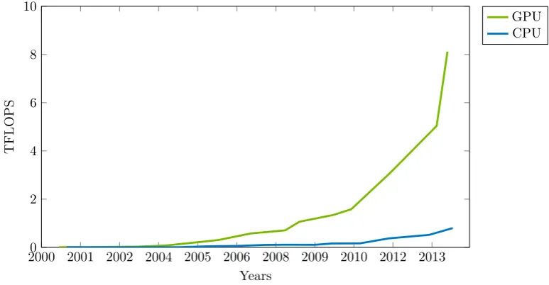
Figure 5 shows the aggregated results of the best CPUs and GPUs, in terms of FLOPS, back to the

year 2000 (NVIDIA Corporation, 2015). The scale on the y-axis is in TFLOPS (1012 FLOPS). It can

be seen that the computational throughput of GPUs is far superior to CPUs. It is for this reason that accelerating MC methods on modern GPUs could be advantageous.

2000 2001 2002 2004 2005 2006 2008 2009 2010 2012 20130

2 4 6 8 10

Years

TFLOPS

GPU CPU

Figure 5: Graph comparing the computational throughput of the best CPUs and GPUs back to the millennium (NVIDIA Corporation, 2015).

4.3.1. CUDA

The CUDA programming framework enables GPUs to be used for general programming tasks. GPUs which are not being used in their traditional role are referred to as GPGPUs. For clarity in this study, the physical processing unit is referred to as a GPU, however when using it in a non-traditional role, as in this study, it is known as a GPGPU.

array is fewer than the threads available, this effectively means that the time taken to carry out the operation on every element in the array is the same as to perform one operation in serial mode.

Programming with CUDA has become more user-friendly and accessible to those who code in C

or C++. The latest iterations of CUDA can hook directly into the users Integrated Development

Environment (IDE) and includes a CUDA debugger as well as code profiler. Writing functions to be performed on the GPGPU are known as kernels. The kernels accept a limited form of the C language, however more features are being introduced with every iteration of the CUDA programming framework (NVIDIA Corporation, 2015).

4.3.2. Grids, Blocks and Threads

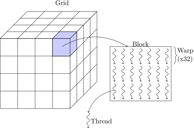
Modern GPUs can have thousands of compute cores and are organised into groups for easier man-agement. The Tesla K40 used in this study has a total of 2,880 cores organised into 15 groups, known as Next Generation Streaming Multiprocessor Units (SMXs), each with 192 cores. As mentioned in Section 4.1, the number of cores contained within a processing unit do not dictate the maximum number of calculations that can be completed in an instance. This is because of industry developments which means that cores are able to perform more than one calculation in an instance depending on the type of operation (Preis et al., 2009). For this reason the number of “threads” are used rather than cores.

In the CUDA programming model, threads are the individual compute entities that carry out the calculations. Groups of threads are known as blocks which have a maximum of 1,024 threads. Threads are launched in multiples of 32 known as a warp e.g. a block of 512 threads is arranged as 16 warps. In more recent iterations of the CUDA framework, a grid of blocks can be sent to the GPGPU for calculation. Depending on the compute capability of the GPGPU, 3 dimensional grids of blocks can be launched. The way these compute units are grouped is illustrated in Figure 6.

Grid

Block

Thread

Warp (x32)

Each grid dimension can accommodate up to 65,536 blocks. For example, the maximum number of threads that can be launched on the Tesla K40 can be seen in Equation 2. This device is capable of 3 dimensional grids where each dimension can have a maximum of 65,536 blocks. Each block can have a maximum of 1,024 threads. Depending on the complexity of the operations being called, the CUDA cores will map one or more of these threads to themselves (Kirk and Hwu, 2010).

M ax. T hreads= 655363·1024 = 2.88·1017 (2)

4.3.3. Coding for GPGPUs

The architecture of a modern computer is such that the CPU and Random Access Memory (RAM) are in constant communication, known as the “host” in the CUDA programming model. When com-puting on the GPGPU, known as the “device” in the CUDA programming model, the host must send the kernel instructions as well as the data required for computation. The process of this is usually:

1. create/load the data on the host

2. allocate space for the data on the device 3. copy the data over to the device

4. launch the kernel on the device

5. copy the data back from the device to the host and finally 6. free the device memory.

The communication between the host and device is through the Peripheral Component Interconnect Express (PCIe) lanes of the computer. Although the bandwidth of these lanes has improved (Ajanovic, 2008), transferring data between the host and device is still time in which no computation is being carried out. Therefore, when coding for GPGPUs it is imperative that the data transfer be as efficient as possible (Sanders and Kandrot, 2010).

On the subject of GPGPU memory, there are various types of memory and each has its own purpose. The global memory has a large allocated space. However, data from global memory is retrieved much slower in comparison to the other memory types. The cache memory and registers are the fastest types of memory. However, the size of these memory types is restricted. By reducing the amount of data as much as possible and focusing on the most valuable data, it will enable more efficient use of the cache and registers. Data in the cache/register is able to be retrieved much faster compared to the global memory which can increase computational throughput.

occurs when, for instance, an IF statement is provided in the code where some members of the warp satisfy the IF statement and others do not. In this instance the warp is split into two branches where each branch executes their sections in serial. This can be a serious performance limitation and so branching should be avoided if possible.

4.4. Generating Random Numbers

MC methods require the generation of many random numbers. An efficient method for generating random numbers is essential to avoid computational slowdown. This is even more apparent after parallelisation because of the relative time of computation. As is usually the case with computation of random numbers on computers, a Pseudo Random Number Generation (PRNG) is used. General methods of using GPGPUs with PRNGs are: (1) if the quantity of random numbers is pre-determinable, a kernel can be written where each thread generates one or more random numbers storing them in an array. A common technique for this method is to use the individual thread ID as the seed value for the PRNG. (2) For situations when the quantity of random numbers is not pre-determinable, the PRNG can be built directly into the simulation algorithm. This way the random numbers can be generated on command.

A third approach was outlined for use in this study but was not required. This approach was for situations when the number of simulations required was not maximising the capability of the GPGPU. This approach used concurrent kernels working in collaboration. The kernel A would control the threads carrying out the simulation. The idle threads would report to the second kernel, B, which would have them generate and upkeep a pool of random numbers. The pool of random numbers would be used by the threads in kernel A, effectively reducing the amount of time the simulation would take as the time needed for getting a random number would simply be its selection from a pre-populated array. The threads in kernel B would keep the array filled with fresh random numbers until the simulations in kernel A had completed.

Before the CUDA framework had matured, those who required random numbers in their CUDA kernels had to develop their own method (Preis et al., 2009). The current CUDA framework includes a tool-kit for PRNG called “cuRAND” which includes many popular PRNG algorithms. In more recent iterations of cuRAND, the Mersenne Twister algorithm has been introduced which has become almost a de facto standard for PRNG (NVIDIA Corporation, 2010). However, its characteristic long period and large state size (Matsumoto and Nishimura, 1998) created difficulties when porting the algorithm over to GPGPUs. This is because GPGPUs work best with lightweight instructions and more complex PRNGs can reduce performance. The default PRNG in cuRAND is the XORWOW algorithm, created by Marsaglia (2003).

Twister. In terms of throughput (random numbers generated per second), XORWOW had better per-formance than the Mersenne Twister algorithm. Finally, the quality of the random numbers generated was tested in the TestU01 Library, a standard PRNG benchmarking suite. In this battery of testing, the Mersenne Twister failed two of the tests and the XORWOW algorithm failed three of the tests. Overall, the default cuRAND PRNG, XORWOW, seems to be better in situations where speed and lightness of weight are required. In problems where the quality of the random numbers is paramount, the Mersenne Twister algorithm is still recommended.

5. GPGPU-Optimised Algorithm for Petri-Net Simulation

Although there are studies in which PNs have been accelerated with GPGPUs, there are no examples in literature of asset management PN models being accelerated with GPGPUs. These represent a different challenge for GPGPU acceleration due to their increased complexity using advanced transitions with decision making capabilities (Le and Andrews, 2016). Additionally, there is evidence that GPGPUs are not able to accelerate all types of problems with the main issues being: (1) highly branched applications, (2) applications with large amounts of data causing memory latency mismatches and (3) imbalanced workloads as would be experienced with MC-based PN samples (Che et al., 2013; Lee et al., 2010).

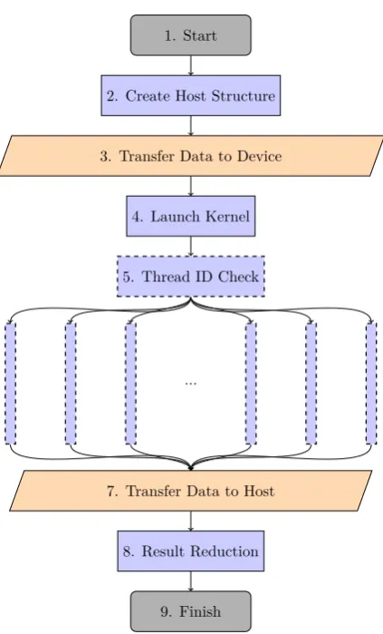
Designing a PN simulation algorithm to take advantage of the benefits of GPGPUs, but avoid the pitfalls, can be complex. An example GPGPU PN algorithm can be seen in Figure 7. The algorithm begins with creating the data on the host device, in this case containing the information to form the PN. Due to the CUDA framework being built on the C language, a common way of containerising the data is to use a structure-of-arrays or an array-of-structures, depending on the data access type of the problem.

The movement of data from the host to the device (stage 3 of Figure 7) can be wasteful as during this time, no computation is being carried out. Therefore, minimisation of the data being transferred can help with the computation time. In the context of PNs, each thread may need the complete set of data to construct the PN. This can be an expensive process as the same set of data would have to be moved to the device for each thread. However, it is possible to utilise the “constant memory” bank of the device. Data in this region is marked as read-only and has the advantage of being able to distribute the data to the threads much quicker. Therefore, with PNs, it may be beneficial to hold the structure of the PN in constant memory so that each thread can access that base information quickly, whilst holding the individual MC sample data within the threads personal memory.

approach is often the slowest configuration as with so many blocks opening and closing, the majority of the time is spent performing housekeeping on the device. The next most common approach is to try to launch as few blocks at once with the maximum number of threads, in this example the configuration would be 1 block with 1000 threads. The thread-centric approach is faster than the block-centric approach but still suffers from low computational efficiency. Often the best launch configuration occurs when the threads have enough to compute to mask the opening/closing overhead, but not too much that they get bogged down with computation. This will often be problem specific, however it was found for the Tesla K40 used in this study that a product of blocks and threads that equalled 15,360 resulted in the quickest computation. This happens to be equal to the 15 SMX cores found in the Tesla K40 multiplied by 1024, the maximum number of threads which can be launched in a kernel.

Step 5 of Figure 7 mentions the thread ID check. This is an important step to avoid a thread trying to access elements of an array which do not exist. This step is required because: (1) threads are launched in groups of 32 known as warps, (2) all threads in a warp execute the same instructions and (3) the CUDA framework uses the C language where arrays are a popular container type. Therefore, if 1000 threads were requested, the GPGPU would launch the nearest multiple of 32 threads that satisfies the users request, in this case 1024 threads. The excess 24 threads would try to execute the same instructions as the rest of the warp, however if there was any attempt at reading from or writing to an array which had a size of 1000, there would be an error. Therefore, it is very common in CUDA kernels to implement a thread ID check where any threads whose ID was greater than 1000 would be ignored. The parallel execution seen in Figure 7 represents the PN sample simulations being executed on the GPGPU. Each of these simulations would carry out the same set of processes as seen in stages 4 through 10 of Figure 1. However, one of the most important aspects when designing an algorithm for GPGPU acceleration is to keep the code as lightweight as possible; i.e. to optimise and make the code as simple as possible. Therefore, it may be necessary to try to reduce the number of PN functions to minimise branching. For instance, for PNs which contain two types of transitions: (1) those with a fixed time period and (2) those which are stochastic; it may be beneficial to try to convert them and use single type transitions that yield similar results. For example, one may prioritise carefully calibrated stochastic transitions over standard fixed time transitions. In this example, the fixed time transitions may be converted to stochastic transitions with a similar behaviour. Performing this operation would speed up computation because it would avoid an IF statement for each transition and consequently possible branching occurrences whilst maintaining similar model behaviour.

average value.

1. Start

2. Create Host Structure

3. Transfer Data to Device

4. Launch Kernel

5. Thread ID Check

...

7. Transfer Data to Host

8. Result Reduction

9. Finish

Figure 7: A schematic demonstrating how a PN algorithm could be devised for GPGPU execution. Nodes with solid outlines are performed on the host. Nodes with dashed outlines are performed on the device.

6. Simple Petri-Net Example

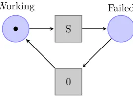
As a proof of concept, the simulations of a simple PN were accelerated using a GPGPU. The PN can be seen in Figure 8; it contains two places, two transitions and a token. The PN represents an asset failing and then being repaired. The transition marked “S” is a stochastic transition and models the failing of an asset represented by a probabilistic distribution. A fixed time transition is used to represent repair of the asset. In this example, the stochastic transition was calibrated with the exponential distribution with a lambda value of 0.035. The fixed time transition represented an instant repair. The sample was simulated for the equivalent of 100 years. The number of samples (1·108) was

chosen to provide enough time for the processing units to stabilise in their clock speeds.

The results of the analysis can be seen in Table 2. ID A1 shows the results of the PN simulated on a single CPU core. For this study a standard quad core desktop CPU was used. The time taken for a single CPU core was 12.89 seconds. This was measured using the C++standard library timing functions.

Working _Failed S

0

Figure 8: A simple PN accelerated with a GPGPU as a proof of concept .

A2). The parallelisation across multiple cores is not directly related to the single core performance, this is because there are overheads in opening, closing and controlling multiple threads.

As mentioned in section 4.2, the individual cores of a GPU are not as robust as a single CPU core. Therefore, when computed on a single GPU core (ID A3) the execution time was 237.8 seconds; almost 20 times slower than with the single core CPU performance. However, when all the GPU cores were enabled (ID A4) the time reduced to 0.085 seconds; over 150 times faster than the single core CPU performance. This result demonstrates the performance gains possible when simulating PNs on GPGPUs.

Table 2: Results of the execution time of a simple PN when computing on various devices.

ID Device Cores Time (s) Speed-up Factor

A1 CPU 1 12.89 1.00

A2 CPU 4 4.481 2.87

A3 GPU 1 237.8 0.05

A4 GPU 2880 0.085 152

7. Railway Bridge Example

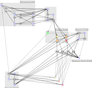
An established railway bridge model has been used as an example in this study. The model is a decision support tool for asset management that is able to predict the condition of railway bridge elements over time, maintenance efforts needed and associated cost. The model itself uses a Coloured Petri-Net (CPN) approach with a number of advanced features. These include both advanced decision making transitions and tuple information held within tokens to identify their attributes. The full model contains 76 places, 108 transitions of which 36 contain advanced decision making functions. A simplified overview of the model can be seen in Figure 9. The details of the full model can be found in Yianni et al. (2016). The full model was was optimised by simplifying its structure and taking into consideration all the suggestions from section 5. The optimised model has a much smaller footprint and is more suited to GPGPU computation.

A1

B2 B3

C2 C3

T1 T2

T3

T4

T5 T6 T7

T8

T10

T9

A1

B2 B3

C2 C3

T13 T14 T15 T16

T11

T12

T17

T18

Deterioration Module

Condition Module Inspection Module

Maintenance Decision Module

Intervention Module

Figure 9: A simplified version of the full railway bridge asset management PN model (Yianni et al., 2016).

states representing the type of defect and the extent of the defect. Here a 2D system of condition states is used to represent the type of the defect and the extent of the defect. This has been calibrated with historical data, provided by Network Rail (NR). As the bridge element deteriorates, there are a number of routes through the 2D condition matrix. The industry guidelines on inspection of railway structures (Network Rail, 2010) has been used to calibrate the inspection module. Depending on the condition of the element, different inspection regimes are required. Elements in better condition require less monitoring whereas those in poorer condition are inspected more frequently. This is reflected in the optimised model too. Once an inspection has taken place, if a repair was required, then the appropriate maintenance action would be selected. The full model includes a number of advanced asset maintenance management features which complicate the PN. A number of these features are included in maintenance decision and intervention modules. More PN features inevitably mean more IF statements in the code which creates occurrences of branching. This has an adverse effect on the computation time of the model. Therefore, in the optimised model these features have been simplified to reduce the branching behaviour. However, the optimised model still conforms to the industry guidelines (Network Rail, 2012). After the intervention, the condition of the element improves accordingly.

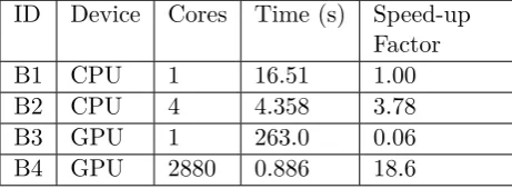
The optimised model was tested on both a CPU and GPU to compare the difference in time. The

Table 3: Results of the execution time of a complex PN when computing on various devices.

ID Device Cores Time (s) Speed-up Factor

B1 CPU 1 16.51 1.00

B2 CPU 4 4.358 3.78

B3 GPU 1 263.0 0.06

B4 GPU 2880 0.886 18.6

first example as this PN is more complex and therefore takes longer to compute. ID B1 presents the results of the single core CPU which totals 16.51 seconds for execution. Again, it can be seen that with multi-core execution (ID B2) the speed-up factor is similar to that found in Table 2 (ID A2). When comparing A3 and B3 from tables 2 and 3; the difference in time is minimal. However, when comparing A4 and B4, it can be seen that there is a significant difference in time. This is because of the sizeable difference in the amount of data needed to construct the PNs. Even though data condensing was carried out, the data must be made available for every thread and this data transfer process extends the overall execution time. The PN profiling revealed that the data transfer process commonly took much longer than the actual compute process; this emphasises the importance of keeping the code and data as lightweight as possible.

8. Conclusion

PNs are becoming increasingly popular in the field of Operations Research (Salimifard and Wright, 2001; Viswanadham and Raghavan, 2000; Aloini et al., 2012). CPNs are also gaining in popularity in this field (Choi et al., 2002; Hosseini et al., 1999; Van Der Vorst et al., 2000). However, it is common for these types of models to require MC-based simulations which can result in long compute times. As modelling approaches grow in complexity, the compute time often follows that. However, with the advancements of GPUs outstripping those of CPUs, acceleration of MC-based simulations is gaining in popularity. Additionally, as time goes on: (1) the development of the CUDA framework makes the features more powerful and user-friendly, (2) the compute performance of GPUs improves and (3) the cost per FLOPS drops. These factors mean that the adoption of GPGPU acceleration should increase dramatically.

One of the main complexities when using GPGPUs is understanding the difference between the processing units of a traditional CPUs and those of a CPUs. Creating code which is lightweight to run, contains minimal data transfers and is parallel in nature has the greatest opportunity for significant acceleration. As GPGPU adoption grows, there is more of a push towards unification of the compute units which will help to mask the boundaries between the host and the device.

stochastic transition was used as a proof of concept. This simple PN was designed to mimic a basic asset transitioning from a working to failed state. Acceleration of this PN resulted in over a 150 times speed-up factor compared to a serial CPU execution.

The purpose of this study was to identify whether acceleration of PN models would be suitable for GPGPUs for decision support tools. As well as identifying their suitability, the process of adaptation for GPGPU acceleration was presented. To that effect, a simple PN was used as a proof of concept with a single stochastic transition. This simple PN was designed to mimic a basic asset from a working to failed state. Acceleration of this PN resulted in over a 150 times speed-up factor from serial CPU execution.

A much more complex PN model for railway bridge asset management was used as the major case study example in this study. The model contained a number of advanced decision making transitions often associated with CPNs. An streamlining exercise was performed on this model to make it more suitable for GPGPU execution, the details of which were documented in section 5. The resulting bridge PN model was accelerated to almost 20 times its original speed. When the accelerated code was profiled, it became apparent that the data transfer from the host to the device was taking the majority of the time; emphasising the importance of minimising data transfers.

The results show that accelerating real-world stochastic PN models with GPGPUs is not only pos-sible, but that the computational improvement is significant. It is possible to accelerate a MC-based PN model to speeds far beyond those found on a traditional CPUs even with a simplistic approach to GPGPU programming. This enhances the applicability of complex PN models which could otherwise be computationally expensive. This technique can therefore be usefully adopted by practitioners to reduce the computational burden of PN model simulations when evaluating alternative asset manage-ment decisions of complex technical systems. This is particularly useful when modern optimisation techniques, requiring repeated simulations of PN models, such as heuristic methods, are employed to inform asset management decisions.

9. Future Developments

feature and would want to know of the most effective techniques for accelerating PNs with GPGPUs. When optimising a full PN model for GPGPU acceleration, the reduction of features often leads to fewer branching situations. However, it may also be possible to re-group the threads of a warp so that one warp will satisfy an IF statement and another will not. In this configuration no branching would have occurred as each whole warp will have diverged down different branches. Therefore, IF statements in the code will have less of an effect on the overall computation time which means the reduction of PN features will not be necessary. In this instance, the optimisation of a full PN model would not result in any loss of functionality.

Finally, in newer versions of the CUDA framework, “streams” have been introduced. This is the ability to use more than one GPU in a computer with modern desktops often being able to handle up to 4 GPUs. This has the ability to speed up computation even further as all of these devices can work concurrently. At the moment these work best with problems that have independent MC samples. However, for larger computational problems, this may be a viable solution. The GPGPU PN algorithm presented in this study could easily be modified to take advantage of a multi-GPU system.

Acknowledgements

John Andrews is the Royal Academy of Engineering and Network Rail Professor of Infrastructure Asset Management. He is also Director of The Lloyds Register Foundation (LRF) Resilience Engineering Research Group at the University of Nottingham. Luis Canhoto Neves is an Assistant Professor in the Resilience Engineering Research Group at the University of Nottingham. Dovile Rama is the Network Rail Research Fellow in Asset management. Panayioti Yianni is a Strategic Consultant within Amey Strategic Consulting and Technology. The research was supported by Network Rail and the Engineering and Physical Sciences Research Council (EPSRC) grant reference EP/L50502X/1. We thank Stephen Greedy, an Assistant Professor in the Faculty of Engineering at the University of Nottingham, for initial advice with coding for GPGPUs. The Tesla K40 used for this research was donated by the NVIDIA Corporation. The authors gratefully acknowledge the support of these organizations.

References

Ajanovic, J., 2008. PCI Express (PCIe) 3.0 Accelerator Features. Intel Corporation, 10.

Aloini, D., Dulmin, R., Mininno, V., 2012. Modelling and assessing ERP project risks: A Petri Net approach. European Journal of Operational Research 220 (2), 484–495.

Andrews, J., 2013. A modelling approach to railway track asset management. Proceedings of the Institution of Mechanical Engineers, Part F: Journal of Rail and Rapid Transit 227 (1), 56–73.

Apodaca, A. A., Gritz, L., Barzel, R., 2000. Advanced RenderMan: Creating CGI for motion pictures. Morgan Kaufmann. Archetti, F., Fagiuoli, E., Sciomachen, A., 1987. Computation Of The Makespan In A Transfer Line With Station

Chalkidis, G., Nagasaki, M., Miyano, S., 2011. High performance hybrid functional Petri net simulations of biological pathway models on CUDA. IEEE/ACM transactions on computational biology and bioinformatics / IEEE, ACM 8 (6), 1545–1556.

Che, S., Beckmann, B. M., Reinhardt, S. K., Skadron, K., Sep. 2013. Pannotia: Understanding irregular GPGPU graph applications. In: 2013 IEEE International Symposium on Workload Characterization (IISWC). pp. 185–195.

Choi, I., Park, C., Lee, C., 2002. Task net: Transactional workflow model based on colored Petri net. European Journal of Operational Research 136 (2), 383–402.

Dagum, L., Enon, R., 1998. OpenMP: an industry standard API for shared-memory programming. Computational Science & Engineering, IEEE 5 (1), 46–55.

Dehnert, J., Freiheit, J., Zimmermann, A., 2002. Modelling and evaluation of time aspects in business processes. Journal of the Operational Research Society 53 (9), 1038–1047.

Geist, R., Crane, D., Daniel, S., Suggs, D., 1994. Systems modeling with xpetri. In: Proceedings of the 26th conference on Winter simulation. Society for Computer Simulation International, pp. 611–618.

Geist, R., Hicks, J., Smotherman, M., Westall, J., 2005. Parallel simulation of petri nets on desktop PC hardware. In: 2005 Winter Simulation Conference, December 4, 2005 - December 7, 2005. Vol. 2005 of Proceedings - Winter Simulation Conference. Institute of Electrical and Electronics Engineers Inc., pp. 374–383.

Hirel, C., Tuffin, B., Trivedi, K. S., 2000. Spnp: Stochastic petri nets. version 6.0. In: Computer Performance Evaluation. Modelling Techniques and Tools. Springer, pp. 354–357.

Hoare, C. A. R., 1978. Communicating sequential processes. Springer.

Hosseini, M., Kerr, R., Randall, R., 1999. Hybrid maintenance model with imperfect inspection for a system with deteri-oration and Poisson failure. Journal of the Operational Research Society 50 (12), 1229–1243.

Hunt, D., Mar. 1995. Advanced performance features of the 64-bit PA-8000. In: Compcon ’95.’Technologies for the Information Superhighway’, Digest of Papers. pp. 123–128.

Jensen, K., Kristensen, L. M., 2009. Coloured Petri nets: modelling and validation of concurrent systems. Springer. Kirk, D., Hwu, W.-M. W., 2010. Programming Massively Parallel Processors. Springer Verlag Gmbh.

Le, B., Andrews, J., Apr. 2016. Modelling wind turbine degradation and maintenance. Wind Energy 19 (4), 571–591. Lee, V. W., Kim, C., Chhugani, J., Deisher, M., Kim, D., Nguyen, A. D., Satish, N., Smelyanskiy, M., Chennupaty, S.,

Hammarlund, P., Singhal, R., Dubey, P., 2010. Debunking the 100X GPU vs. CPU Myth: An Evaluation of Throughput Computing on CPU and GPU. In: Proceedings of the 37th Annual International Symposium on Computer Architecture. ISCA ’10. ACM, New York, NY, USA, pp. 451–460.

Marsaglia, G., 2003. Xorshift rngs. Journal of Statistical Software 8 (14), 1–6.

Matsumoto, M., Nishimura, T., 1998. Mersenne twister: a 623-dimensionally equidistributed uniform pseudo-random number generator. ACM Transactions on Modeling and Computer Simulation (TOMACS) 8 (1), 3–30.

Nandapalan, N., Brent, R. P., Murray, L. M., Rendell, A. P., 2011. High-performance pseudo-random number generation on graphics processing units. In: Parallel Processing and Applied Mathematics. Springer, pp. 609–618.

Network Rail, 2010. Handbook for the examination of Structures Part 2A: Bridges. NR/L3/CIV/006/2A. Network Rail, 2012. Policy on a Page: Structures.

NVIDIA Corporation, 2010. CURAND library.

NVIDIA Corporation, 2012. Thrust Quick Start Guide. NVIDIA. NVIDIA Corporation, 2015. CUDA C Programming Guide.

Petri, C. A., 1962. Communication with Automation. Ph.D. thesis, Mathematical Institute of the University of Bonn, Bonn, Germany.

Preis, T., Virnau, P., Paul, W., Schneider, J. J., 2009. GPU accelerated Monte Carlo simulation of the 2D and 3D Ising model. Journal of Computational Physics 228 (12), 4468–4477.

Engineers, Part F: Journal of Rail and Rapid Transit 227 (4), 344–363.

Salimifard, K., Wright, M., 2001. Petri net-based modelling of workflow systems: An overview. European Journal of Operational Research 134 (3), 664–676.

Sanders, J., Kandrot, E., 2010. CUDA by Example: An Introduction to General-Purpose GPU Programming, Portable Documents. Addison-Wesley Professional.

Schaller, R. R., 1997. Moore’s law: past, present and future. Spectrum, IEEE 34 (6), 52–59. Schneeweiss, W. G., 2004. Petri Net Picture Book. LiLoLe Verlag GmbH.

Tomov, S., McGuigan, M., Bennett, R., Smith, G., Spiletic, J., Feb. 2005. Benchmarking and implementation of probability-based simulations on programmable graphics cards. Computers & Graphics 29 (1), 71–80.

Van Der Vorst, J. G., Beulens, A. J., Van Beek, P., 2000. Modelling and simulating multi-echelon food systems. European Journal of Operational Research 122 (2), 354–366.

van Meel, J. A., Arnold, A., Frenkel, D., Zwart, S. F. P., Belleman, R. G., 2008. Harvesting graphics power for MD simulations. Molecular Simulation 34 (3), 259–266.

Viswanadham, N., Raghavan, N. S., 2000. Performance analysis and design of supply chains: A Petri net approach. Journal of the Operational Research Society 51 (10), 1158–1169.

Yang, J., Wang, Y., Chen, Y., Feb. 2007. GPU accelerated molecular dynamics simulation of thermal conductivities. Journal of Computational Physics 221 (2), 799–804.