Nonequilibrium effective field theory for absorbing state phase transitions in driven
open quantum spin systems
Michael Buchhold,1Benjamin Everest,2,3Matteo Marcuzzi,2,3Igor Lesanovsky,2,3and Sebastian Diehl1
1Institut f¨ur Theoretische Physik, Universit¨at zu K¨oln, D-50937 Cologne, Germany
2School of Physics and Astronomy, University of Nottingham, Nottingham, NG7 2RD, United Kingdom 3Centre for the Mathematics and Theoretical Physics of Quantum Non-Equilibrium Systems, University of Nottingham,
Nottingham, NG7 2RD, United Kingdom
(Received 14 November 2016; revised manuscript received 10 January 2017; published 27 January 2017) Phase transitions to absorbing states are among the simplest examples of critical phenomena out of equilibrium. The characteristic feature of these models is the presence of a fluctuationless configuration which the dynamics cannot leave, which has proved a rather stringent requirement in experiments. Recently, a proposal to seek such transitions in highly tunable systems of cold-atomic gases offers to probe this physics and, at the same time, to investigate the robustness of these transitions to quantum coherent effects. Here, we specifically focus on the in-terplay between classical and quantum fluctuations in a simple driven open quantum model which, in the classical limit, reproduces a contact process, which is known to undergo a continuous transition in the “directed percolation” universality class. We derive an effective long-wavelength field theory for the present class of open spin systems and show that, due to quantum fluctuations, the nature of the transition changes from second to first order, passing through a bicritical point which appears to belong instead to the “tricritical directed percolation” class. DOI:10.1103/PhysRevB.95.014308
I. INTRODUCTION
The dynamics of many-body systems is typically too complex to admit a complete description. It is well known, however, that for systems at thermal equilibrium, time-averaged, macroscopic quantities (i.e., quantities which do not react to fluctuations on microscopic time and length scales) can be equivalently extracted from appropriate statistical en-sembles [1,2]. Statistical mechanics provides a very powerful simplification which recasts all the relevant physics in terms of a few thermodynamic parameters and potentials independently of the initial state of the system, although one could envision cases in which some initial state information is kept due to an extensive amount of symmetries, and the ensembles would have to be generalized accordingly [3–5].
Equilibrium systems, however, are but a portion of what nature has in store. Despite significant efforts, a thorough, systematic understanding of nonequilibrium phenomena has yet to be developed. As in equilibrium, though, there are cases in which collective behaviors supersede the minute details of the microscopic dynamics, allowing their description in terms of few coarse-grained variables and rules. One example is given by cooperative relaxation at the onset of glassiness [6,7] in which, e.g., it is not possible to change the local configuration of particles without an extensively growing number of rearrangements in the neighborhood taking place. Another relevant instance relies on the presence of continuous phase transitions [8–11]. These are associated to a diverging length in the correlations of fluctuations [8,12,13]. Hence, fluctuations encompass larger and larger portions of the system as the critical point is approached, so that they end up being governed only by general features which do not depend on the scale, such as dimensionality and symmetries. This idea lies at the basis of the concept ofuniversality; simply put, all systems sharing these scale-insensitive features will display quantitatively identical behavior at asymptotic distances, and studying one instance will provide information on all of them.
It is therefore a relevant task to identify and study phase transitions as they provide a natural classification scheme.
In dynamical systems, a crucial distinction must be made depending on whether detailed balance conditions, or the associated symmetrymicroreversibility[14–17], hold or not. In the former case, the system will evolve towards a stationary equilibrium state. Examples of this kind are systems subject to an external thermal bath, which have been extensively investigated and classified [18]. It is worth remarking that this symmetry might be absent from the microscopic description, but be effectively recovered under coarse graining at long times and long wavelengths [19–21]. If this is not the case, the system will instead remain out of equilibrium even in the long-time limit, being typically described byflux equilibriumstates [22]. Phase transitions in this regime will have no equilibrium coun-terpart but are genuinely nonequilibrium in nature [11,23].
following asbranching. This can be summarized as
↑−→ ↓γ , ↑↓−→ ↑↑κ . (1.1) As their name suggests, inactive sites do not produce any dynamics. The configuration where all sites are inactive thus cannot be left and constitutes the unique absorbing state of the model. Note that the two processes in Eq. (1.1) are competing: decay tends to deplete the system of↑’s, whereas branching tries to fill it up. In the thermodynamic limit, depending on the ratioκ/γ between the rates, the dynamics starting from an active configuration can end up in two distinct phases: forκ γdecay dominates and the system at long times invariably falls into the absorbing state. Forκ γ, instead, a finite density of active sites persists for arbitrarily long times and the dynamics survives in the transient portion of the phase space. Note that this is only strictly true in the thermodynamic limit: for any finite size, there is always a finite probability of a (rare) fluctu-ation trapping the system into its absorbing state. In the active phase, however, the time required for such a fluctuation to take place increases with the system size [28]. The active and ab-sorbing phases are separated by a critical pointκc/γc, marking
the directed percolation (DP) transition [24], with the station-ary densitynof active sites acting as an order parameter (i.e.,
n=0 in the absorbing phase versusn >0 in the active one). The directed percolation class is conjectured [29,30] to en-compass all systems featuring a one-component order param-eter, short-range interactions, no additional symmetries, and a unique, fluctuationless absorbing state. This last condition is crucial; the difficulty in having a perfectly fluctuation-free state in real systems has made it a challenge to identify experimental setups undergoing a phase transition in this class [31]. The first clear examples have only recently been highlighted in two-dimensional nematic liquid crystals [32,33] and one- [34] and two-dimensional [35] turbulent flows. In addition, a recent numerical study links DP to the onset of turbulence in quantum fluids (such as superfluids) [36]. Upon relaxing the other assumptions, different transitions, alongside their universality classes, have been identified and investigated: for instance, the introduction of quenched spatial randomness [37–39] makes the DP critical point unstable (it constitutes a “relevant” perturbation in the renormalization group sense) and generates nonuniversal power laws; the presence of multiple absorbing states often leads to the appearance of discontinuous transitions [40,41]; other symmetries, such as preservation of the parity of active sites [42,43], also change the critical properties, as does introducing long-range processes (L´evy flights) [44]. As in equilibrium systems, multicritical behavior can emerge when higher-order processes take over the simple ones in Eq. (1.1) [45,46]. A simple example studied in the literature is the so-called tricritical directed percolation [30,47,48], obtained, e.g., by adding processes involving pairs such as↑↑↓ → ↑↑↑or ↑↑ → ↓↓. Depending on the relative rates of these processes compared to the ordinary DP ones, the transition may become first order by crossing a bicritical point.1
1The term “tricritical directed percolation” has been established in
the literature. The critical point, however, separates two distinct stable phases of matter and is thus according to the statistical mechanics definition a bicritical point.
Recently, a proposal [49] has been made to realize DP with cold-atomic gases excited to high-lying electronic orbitals (so-calledRydberg states [50,51]). This yields greatly enhanced dipolar or van der Waals mutual interactions [52,53], which can easily produce strong correlations and in fact induce several examples of collective behaviors [54–58]. In particular, they make it possible to engineer a facilitation mechanism [59–61], where atoms lying at a certain distance from already-excited ones have a much higher probability of getting excited, thereby reproducing a branching process (rateκabove) [62,63]. Spon-taneous radiative decay provides the competing process (rate
γabove). A strong dephasing noise projects the dynamics onto an effective classical master equation [64,65], although the mi-croscopic dynamics is properly described by a quantum master equation. Quantum driven-dissipative systems such as this one currently attract great theoretical interest [17,21,66–70] and have been investigated in a broad spectrum of exper-imental setups, including, e.g., light-driven semiconductor heterostructures [71], arrays of driven microcavities [72,73], and cold atoms in optical lattices [74] and cavities [75,76]. These systems share in common that the microscopic processes governing the driving and dissipation explicitly break detailed balance, pushing these systems out of equilibrium [17,21]. However, as mentioned above, equilibrium conditions can be recovered on mesoscopic time and length scales upon coarse graining and this turns out to be indeed the case in several instances [19,66,68,77]; from a physical perspective, this is due to the “fast” degrees of freedom acting as an effective thermal bath for the “slow” ones [78,79]. However, examples have been identified in which not only the nonequilibrium nature [80,81], but also the quantum coherent aspects [82,83] of the dynamics persist under rescaling to arbitrarily long wavelengths. The proposal outlined above then opens up a new path to explore, i.e., to check the robustness of DP under the influence of quantum fluctuations in regimes which are not dominated by the dephasing noise. This question was addressed in Ref. [84] via an effective action approach; it was found that, while the nature of the transition from the absorbing phase to the active one does not change when the quantum terms are small compared to the classical ones, it instead switches to discontinuous (first order) in the opposite regime.
A. Overview and key results
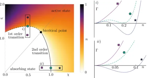
FIG. 1. Mean field phase diagram of the quantum contact process. The system can undergo a phase transition from an absorbing state towards an active, nonzero density phase, which can be either continuous (solid line) or first order (dashed line). The second-and first-order lines meet at a bicritical point. The axes represent the rescaled classical branching rate χ=zκ/γ and the quantum branching rateω=z/γ and correspond to the classical (A) and quantum (B) limits, respectively. The dotted diagonal line indicates the competing regime (C). On the right, the corresponding evolution of the potential as a function of the axes’ parameters is shown for (i) the first-order transition and (ii) the second-order transition.
transformation (see, e.g., Ref. [86]), do not preserve this constraint and thus do not constitute a viable option in our case. Technically, we first recast the quantum master equation into noisy Heisenberg equations for the three onsite spin operators
σix,y,z. The resulting equations of motion are decoupled at the mean field level, which accounts for the short distance physics of the problem. These equations feature two gapped and one potentially gapless variable, the latter being associated with density fluctuations. We then map the problem into a Martin-Siggia-Rose-Janssen-de Dominicis (MSRJD) functional integral.
After elimination of the gapped fluctuations, we end up with a description in terms of a dynamical action for the density variable alone. In the limit where the coherent microscopic processes vanish, we reproduce the action governing the DP universality class, so that our procedure represents one of the rare instances where the DP action is derived from a concrete microscopic model. Incorporating the “quantum scale” associated to the coherent branching process introduces a new relevant parameter in the problem on the microscopic level, and leads to important structural modifications of the DP action, among them, an interaction parameter may cross zero and change sign, signaling a critical end point of a second-order phase transition, which afterwards turns into a first-order one. Moreover, the defining rapidity inversion symmetry of DP is broken in our model. On the other hand, the second key structural property of DP, the existence of an inactive state, signaled by a noise level that scales to zero with the density, is still present in our long-wavelength theory.
Structure and key properties of the phase diagram. The phase diagram of our model is depicted in Fig.1. The additional quantum scale, describing coherent branching, adds a relevant parameter to the problem and is thus expected to give rise to an additional phase transition in the problem. Indeed, a new first-order phase transition is found in the absence of incoherent
branching. Increasing the incoherent branching gives rise to a critical end point, manifestly characterized by different symmetries than DP, and therefore giving rise to a distinct universality class. The corresponding long-wavelength action in the vicinity of the bicritical point resembles the effective action for the so-called “tricritical directed percolation” class. In order to assess the physics of the new (bi)critical point and the first-order transition, we elaborate as follows:
(i) Nature of the bicritical point phase transition. We compute a set of critical exponents, determining the univer-sality class, of the bicritical point. To this end, we develop a background-field functional RG method approaching the phase transition from the active side, based on previous work benchmarked for the DP universality class [87]. This approach is capable of effectively incorporating higher-loop effects, which turns out to be crucial at the bicritical point. We furthermore deliver an exact RG argument for the protection from the generation of an additive Markovian noise level term. Remarkably, this substitutes the usual symmetry-based argument due to the presence of rapidity inversion symmetry, which we cannot rely on in the presence of coherent branching. Finally, we estimate the Ginzburg scale for the extent of the critical domain near the phase transition. As expected, its range increases substantially when lowering the dimension.
(ii) First-order transition. We investigate the properties of the first-order nonequilibrium phase transition in a ho-mogeneous optimal path approximation. A remarkable trait of the analysis is that, despite the problem is manifestly out of equilibrium due to the special nature of the noise, we are still able to construct a stationary, non-Gibbsian probability distribution within our approximations. The role of the density-dependent noise is to stabilize the inactive phase with respect to what an analogous, but field-independent, noise would do. In addition, we estimate finite-size effects, and find that systems of around 5000 lattice sites should suffice to see a clear discontinuity, evidencing the first-order nature of the phase transition. We note that this approach gives a rough idea on the physics of the first-order transition only. It discards explicitly instantonlike, spatially inhomogeneous field configurations, that should play a role at least close to the transition. Surprisingly little is known on nonequilibrium first-order transitions, and we reserve an in-depth study of this problem for future research.
Physical implementation. We furthermore discuss an idea for implementing the considered physics with the help of atomic lattice systems in which interacting Rydberg states are excited both coherently and incoherently. This could provide a guide for current experiments to address the competition between classical and coherent processes in nonequilibrium phase transitions.
This paper is structured as follows: In Sec.IIwe introduce the microscopic model and derive the effective functional integral description for its dynamical properties; in Sec.III
Monte Carlo techniques before providing our concluding remarks (Sec.VII).
II. MICROSCOPIC MODEL AND DENSITY ACTION FUNCTIONAL
We consider here thequantum contact processoriginally introduced in Ref. [84], which is defined on ad-dimensional square lattice with spacing a. For simplicity, we label the sites with a single index l=1. . .N; each individual site is a two-level quantum system which can be either active (|↑l) and contribute to the dynamics or inactive (|↓l) and
remain inert until activated. In the Rydberg-atom language of Ref. [49], these would correspond to an excited atom and a ground-state one, respectively. Note that, in contrast to the classical contact process, here we admit generic coherent superpositionsαl|↑l+βl|↓lwith|αl|2+ |βl|2=1.
The dynamics is defined in terms of the following processes: (i) Decay: Active sites are spontaneously inactivated at a rateγ (|↑→ |↓).γ
(ii) Classical branching/coagulation: To mimic the facil-itated dynamics introduced above, we consider incoherent activation at rateκof sites neighboring an excitation (|↑↓→κ |↑↑), but we also account for the time-reversed process, i.e., facilitated inactivation orcoagulation occurring at the same rate (|↑↑ κ
→ |↑↓). In our current conventions, the actual rates are proportional to the numberNAof active neighbors,
e.g.,|↑↓↑←→ |↑↑↑.2κ
(iii) Quantum branching/coagulation: We introduce a HamiltonianH (see further below) which connects precisely the same states connected by classical branching and coag-ulation, i.e., such that a|H|b =NAif|a
NAκ
←→ |b(and, in particular, a|H|b =0 if NA=0), being an overall
coefficient fixing its amplitude. The example above translates here to ↑↓↑|H|↑↑↑ =2.
The third process is the minimal quantum equivalent of the second one and provides the quantum competition to the purely classical process. It is also important to remark that (i)–(iii) preserve the fundamental property of DP, i.e., the presence of a unique absorbing state corresponding to the fully inactive one|abs = ⊗l|↓l. In order to describe the dynamics of this
quantum contact process, we will discuss the corresponding microscopic Heisenberg-Langevin equations and derive an effective long-wavelength nonequilibrium path-integral de-scription. The latter is particularly well suited to describe the dynamics close to the active-to-inactive, i.e., the absorbing state, phase transition.
A. Microscopic model
The ideal model presented above is a driven open quantum lattice of spin-12 variables. In order to define it formally, it is convenient to introduce here a complete set of spin operators acting on sitel,
σl+= |↑l ↓|l, σl−= |↓l ↑|l, and
σlz= |↑l ↑|l− |↓l ↓|l (2.1)
or, equivalently,
σlx =σl++σl−, σly= −iσl++iσl−, and
nl =σl+σl−= |↑l ↑|l. (2.2)
In particular,nl is the local projector onto an active site, i.e.,
nl|↑l= |↑landnl|↓l=0. Its global expectation valuen=
(1/N)l nlwill constitute our order parameter. As we are
considering only Markovian processes as appropriate for these systems [21], the time evolution of the system’s density matrix
ρis given by a quantum master equation [88,89]
∂tρ=Sρ = −i[H,ρ]+
l
L(d) l ρ+
l
L(b) l ρ+
l
L(c) l ρ.
(2.3)
We have introduced the shorthand S for the superoperator acting on the density matrix ρ for future reference. The coherent part (iii) is encoded in the Hamiltonian
H =
l
lσlx with l=
mnnl
nm, (2.4)
where “nn” denotes a summation restricted to nearest neigh-bors only. The operator l “counts” the number of active
nearest neighbors of l and enforces the constraint of at least one excitation being present for being able to flip site
l. Processes (i) and (ii) are instead accounted for via the Liouvillians L(i), i=d,b,c, with the apices distinguishing
between those contributing to decay (d), classical branching (b), and coagulation (c). The Liouvillians are each generated by a set of Lindblad or quantum-jump operatorsL(i)m, and take the standard Lindblad form [88,89]
L(i)ρ = m
L(i)mρL(i)m†−1
2
L(i)m†L(i)m,ρ, (2.5)
which ensures preservation of probability and positivity. For the dissipative processes considered, the jump operators read as
L(d)l,m≡L(d)l =√γσl−, (2.6a)
L(b)l,m=√κnmσl+, (2.6b)
L(c)l,m=√κnmσl−, (2.6c)
so that we find
L(d)
l ρ =γ σl−ρσl+−12{nl,ρ}
(2.7)
for spontaneous decay,
L(b) l ρ=κ
mnnl
nmσl+ρnmσl−−
1
2{nm(1−nl),ρ}
(2.8)
for classical branching, and
L(c) l ρ=κ
mnnl
nmσl−ρnmσl+−
1
2{nmnl,ρ}
(2.9)
to leading order in /γdeph, to a classical master equation
which can be described via a set of jump operators
L(H)l =
42
γdeph
l(σl−+σl+), (2.10)
which only differ from the ones in Eqs. (2.6b) and (2.6c) by the fact that, in the presence of NA active neighbors,
the rate of “facilitated flipping” is enhanced quadratically (4N2
A2/γdeph), instead of linearly (NAκ). However, at the
critical point the density of active sitesnvanishes; therefore, the critical properties are dominated by configurations in which
NA remains low on average. In particular, if NA1, then
NA2 ≈NA, since typically it mostly takes the discrete values 0
and 1. Therefore, this difference can at most shift the critical point and change the profile ofnin the active phase, but cannot modify the universal properties.
B. Heisenberg-Langevin equations
In order to derive a path-integral description for the current model, we will determine the Heisenberg-Langevin equations for the spin operators in this section. These equations represent the equations of motion for the spins in the presence of Hamiltonian and dissipative dynamics and by construction preserve the local spin algebra (see Appendix A for some general aspects of Heisenberg-Langevin equations). The latter is crucial for the correct implementation of the contact process dynamics in terms of local quantum operators. Afterwards, we will perform a mean field decoupling, which approxi-mates the spin operators by local, stochastically fluctuating fields, obeying Langevin equations of motion. The Langevin dynamics will then be recast in terms of a nonequilibrium path integral, which is discussed below. One should note that a Holstein-Primakoff approximation of the master equation and a subsequent mapping of the master equation to a Keldysh path integral, as e.g. performed in Ref. [86], typically replaces the strong constraint on the spin Hilbert space via a soft constraint, which implements the spin algebra not exactly but only on average. This is not sufficient in order to derive a field theory for the contact process and thus the present approach via the Heisenberg-Langevin equations is required instead.
In order to keep our order parameter explicit, we write the Heisenberg-Langevin equations in terms of the set (2.2) of one-spin observables (alongside the identity, they span the entire local Hilbert space of operators). For convenience, we introduce the shorthandsl =
mnnlσmx and the coordination
number z=2d of the lattice, i.e., the number of nearest neighbors per site, where we recall that d is the number of spatial dimensions. The equations of motion (EOM) are derived by applying (A4), which leads to
∂tnl = −γnl+
σly−κ(2nl−1)l+ξln, (2.11)
∂tσlx = −σ y lsl−
κz+γ
2 σ
x l −κσ
x
ll+ξlx, (2.12)
∂tσ y l =σ
x lsl−
κz+γ
2 σ
y l +ξ
y l −
2(2nl−1)+κσ y l l.
(2.13)
Note that Eq. (2.12) differs from Eq. (3) of Ref. [84] by the sign of the first addend (which reads as+σlysl there, once
translated in our present notation). This constitutes a typo which we correct here; the discussion of the phase diagram and critical properties, however, remains completely unaffected, as we shall show in the following. As anticipated above, in order to fix the noise operators we consider a system-bath coupling which, once the bath variables are integrated out in a Born-Markov approximation, yields the same deterministic part of the equations (2.11)–(2.13). We assume that the spatial correlations of the bath are much shorter than the lattice constant a, such that noise correlations between different lattice sites are absent and every lattice site is effectively coupled to its own independent (but identical) environment. This allows us to focus our subsequent analysis on a single site; for simplicity, in the derivation of the noise we will be dropping the position index. The discussion for the general case can be straightforwardly recovered by adding a subscriptl to all system and bath operators. We need three terms to separately account for decay, branching, and coagulation, which will generate contributionsξd,ξb, andξcto the noise, respectively.
We thus introduce the three local HamiltoniansHd,Hb, and
Hc. The former reads as
Hd=
q
λq(σ+dq+dq†σ−)+
q
ωqdq†dq, (2.14)
where thedq operators represent bosonic modes ([dq,dk†]=
δqk), ωq their dispersion relation, and λq their respective
coupling with the spin. Since decay corresponds to photon emission into the vacuum, we assume these modes to be in a stateρ0
d at zero temperature and sufficiently numerous
so that the action of the system on them can be considered negligible (i.e., they can be approximated as a continuum of modes). In order to reproduce the branching and coagulation dynamics above, we actually have to impose a further con-straint, i.e., that there are two independent baths of harmonic oscillators for every pair of neighboring spins. The system-bath Hamiltonians will read as, for a generic (neighboring) pair,
Hb =
k
αknnn(σ−bk+b†kσ+)+
k
νkb†kbk,
Hc=
k
αknnn(σ+ck+c†kσ−)+
k
νkck†ck, (2.15)
where the nn denotes a given neighbor of the site considered, and correspondingly
Hb,nn =
k
αkn(σnn−bk,nn+b†k,nnσnn+)+
k
νkb†k,nnbk,nn,
Hc,nn =
k
αkn(σnn+ck,nn+ck,nn† σnn−)+
k
νkc†k,nnck,nn,
(2.16)
and thebk’s andck’s are bosonic modes with equal dispersions
νkand couplingαk to the spin. These baths are initialized in
equal statesρ0
b/c, to allow excitation and deexcitation of the
We start by considering spontaneous decay. The (ordinary) Heisenberg equations under the action ofHd read as
∂tσ− =i[Hd,σ−]=i
q
λqdqσz, (2.17)
∂tn=i[Hd,n]=i
q
λq(dq†σ−−σ+dq), (2.18)
∂tdq =i[Hd,dq]= −iλqσ−−iωqdq. (2.19)
Equation (2.19) can be formally integrated yielding
dq(t)=dq(0)e−iωqt−iλq
t
0
dtσ−(t)e−iωq(t−t). (2.20)
Inserting (2.20) into (2.18) gives
∂tn(t)= −
q
λ2q
t
0
dt[σ+(t)σ−(t)eiωq(t−t)+H.c.]
+i
q
λq(dq†(0)σ−(t)e
iωqt−σ+(t)d
q(0)e−iωqt)
≈ −γn(t)+i
q
λq(dq†(0)σ−e
iωqt−H.c.)
ξn d
. (2.21)
The first term of Eq. (2.21) is obtained by applying the Born-Markov approximation for a bath, which is fluctuating rapidly on typical system time scales [90]. The effective coupling strengthγ =2π λ2(0)D(0) is proportional to the bath density of states D(ω)=qδ(ω−ωq) and the coupling constants
λ(ω)=qλqδ(ω−ωq) both evaluated at zero frequency.
The second term contains information on the initial state of the bath and is nothing but the desired noise operator. This clarifies the meaning of the noise average . . .ξ, which is
nothing else than the trace over the bath degrees of freedom
. . .ξ =tr
(. . .)ρd0. (2.22)
Sinceρ0
dis a definite-particle-number state, the noise has zero
mean ξdnξ =0. The variance, however, does not vanish and reads as
ξdn(t)ξdn(t)ξ B-M=
q
λ2q[nqeiωq(t−t
)
σ−(t)σ+(t)
+(1+nq)e−iωq(t−t
)
σ+(t)σ−(t)]
B-M
= γ[Nd+n(t)]δ(t−t) (2.23) T=0
= γn(t)δ(t−t). (2.24) Here, we have applied the Born-Markov approximation to commute system and bath variables at different times and employed the shorthandnq = dq†dqξ andNd =
qnq. The
second (approximate) equality comes, as mentioned above, from assuming that the bath fluctuates much faster than the typical system time scales, implying that both spectral densitiesD(ω) andλ(ω) are slowly varying functions of their arguments, such that the summation effectively yields a time-local result. The final equality is exact and comes from the fact that the bath is at zero temperature, hence, dq†dqξ =0 ∀q
and Nd =0. Equation (2.24) highlights the multiplicative
nature of the density noise (ξn d ∼
√
n). This property leads to a noiseless density channel for the empty staten=0, and ensures the absence of density fluctuations in the absorbing state. A small but nonzero temperature of the bathT =0 will instead lead to a nonvanishing bath photon numberNd ∼Td
(valid for relativistic bosonic particles indspatial dimensions) and modify the absorbing state nature of the transition on time scalesτ >(γ Nd)−1∼T−d and distances x >(γ Nd)−1/2 ∼
T−d/2. For sufficiently low temperatures, as achieved by
current cold-atom experiments, these scales are much larger than the system’s and these effects can thus be ignored.
The remaining equation of motion forσ−can be solved in the same spirit of Eqs. (2.21) and (2.24), which yields
∂tσ−(t)= −
γ
2σ
−(t)+i
q
λqdq(0)σz(t)eiωqt
ξd−(t)
. (2.25)
This defines the noise operator ξd−(t) and, via conjugation,
ξd+(t)=[ξd−(t)]†, as well asξx
d =ξd++ξd− andξ y
d =i(ξd−−
ξd+). The complete noise correlations can be determined from Eqs. (2.21) and (2.25), which are straightforwardly extended to the entire lattice by reinstating the position indices. In the (x,y,n) basis [i.e., set (2.2)] the noise correlations can be expressed as
ξd,l(t)ξ†d,l(t)ξ =γ δ(t−t)δl,l
⎛
⎝ 1 −i σ
− l
i 1 iσl−
σl+ −iσl+ nl
⎞ ⎠,
(2.26)
whereξ†d,l(t)=(ξ x d,l(t),ξ
y d,l(t),ξ
n
d,l(t)). As pointed out above,
the noise average . . .ξ represents a quantum mechanical
average over the bath degrees of freedom, such that the entries in Eq. (2.26) remain operator valued. We remark again that the noise is only additive in theσx,y channels, while it remains
multiplicative in the density channel. In the limit κ, the coupling of the density field to the σy matrix can be eliminated and leads to a modification of the branching rate
κ, as mentioned above. In this limit, the Heisenberg-Langevin equation for the density (2.11) has an absorbing configuration for {nl} =0. We will show in the following that the latter
feature persists for all values of and that the {nl} =0
configuration remains an absorbing state for the density channel. Note that, due to our choice of the bath stateρd0, the noise is Gaussian and therefore entirely defined in terms of its mean expectation value and two-point correlations. Due to the Markov approximation, the noise is white (time local) as well. So far, we have not considered the noise contribution from the branching and coagulation dynamics stemming from the Hamiltonian (2.15). Interestingly, there is no need to: as long as we are only interested in the critical properties, we can safely neglect higher orders inn, as they will just provide subleading corrections. Due to the factorsnandnnnin the Hamiltonians
Hb/c andHb/c,nn, we are guaranteed that the noise termsξb
andξcwill never dominate, at low densities, over the decay
noiseξd. Therefore, for simplicity, we can safely neglect their
presence and setξ ≡ξd+ξb+ξc→ξd. For completeness,
Together with the noise kernel (2.26), the Heisenberg-Langevin equations (2.11)–(2.13) represent the starting point for our analysis of the absorbing state phase transition in terms of a nonequilibrium path-integral framework. While the deterministic part of the Heisenberg-Langevin equations is exact, we have approximated the noise kernel up to leading order in the density according to the previous discussion and kept only the decay contribution which still generates all relevant terms.
C. Nonequilibrium path-integral description
In order to investigate the dynamics close to the ab-sorbing state, we derive a nonequilibrium path-integral de-scription for the density variable n. Our method is based on the Martin-Siggia-Rose-Janssen-de Dominicis (MSRJD) approach [10,91–93], a well-established mapping of Langevin equations into effective field theory actions. In order to do this, we therefore first need to reduce our Heisenberg-Langevin equations (2.11)–(2.13) to semiclassical ones. This is achieved via a mean field, site-decoupling approximation (i.e., averages involving operators acting on different sites are factorized, OlOm → Ol Om for l=m), which yields a
set of (deterministic) equations
∂tnl= −γ nl+
σly−κ(2nl−1)
l,
∂tσlx = −σ y lsl−
κz+γ
2 σ
x l −κσ
x
ll, (2.27)
∂tσly =σ x lsl−
κz+γ
2 σ
y l −
2(2nl−1)+κσly
l,
as we recall that bothsl and l act nontrivially only on
the nearest neighbors of l, and not on site l itself. Relying on translational invariance to make a uniform assumption (nl =nm ≡nandσlx/y=σ
x/y
m ≡σx/y ∀l,m) one can further
reduce them to
∂tn=[−γ+z[σy−κ(2n−1)]]n,
∂tσx = −
zσy+κz+γ
2 +κzn
σx, (2.28)
∂tσy =z(σx)2−
κz+γ
2 σ
y−zn
[2(2n−1)+κσy].
The stationary solutions are found by setting the time deriva-tives to 0. Introducing the dimensionless constantsχ=zκ/γ
andω=z/γ, we find that the stationary density of active sites obeys
n(4ω2+2χ2)n2−2(ω2−χ)n+12(1−χ2)=0. (2.29) The solutionn=0 corresponds to the absorbing state, which is always present, but is only dynamically stable forχ <1 (see AppendixF). Forχ >1, instead, any perturbation away from it will grow to reach one of the other solutions, marking the active phase. Forχ <1, the nonabsorbing solutions still exist as long as the discriminant is positive [ω4+χ4+2ω2(χ2−
χ−1)0]. If additionallyω2> χ, a saddle-node bifurcation takes place, corresponding to a first-order phase transition to a coexisting, bistable regime.
The mean field equations (2.27) constitute our starting point. We stress here again that the present approach respects the constrained nature of the local spin Hilbert space, which
is crucial for the correct description of the contact process. This is advantageous over a bosonic Holstein-Primakoff [94] approximation, which introduces a much larger bosonic Hilbert space and does not preserve the local spin constraint, i.e., it allows for an arbitrary number of bosonic excitations being present on each site. In the classical case, it turns out that the latter produces a completely different behavior [85], e.g., if the branching and decay rates are equal, the average density of excitations remains constant. As a consequence, the representation of the spins in terms of Holstein-Primakoff bosons excludes any absorbing dark state, unless the local Hilbert space has a strict upper bound on the number of bosons per lattice site. It is therefore important to keep the “hard core” (or “exclusion”) as a fundamental property of the dynamics. This hard-core constraint promotes any bosonic field theory to a formidable problem to solve and is conveniently avoided by the present approach. Furthermore, the fluctuations induced by the environment must be taken into account in a way that is consistent with the discussion above. In particular, it is crucial to maintain the multiplicative nature of the noise on
n. The variablesnl,σ x/y
l are now real valued and the noise
must be as well. We thus introduce a Gaussian, white noise ξl =(ξ
x l ,ξ
y l,ξ
n
l) with vanishing mean and a covariance matrix
extracted from the Hermitian part of the operator valued one in Eq. (2.26) [see Eq. (2.34) below].
Since continuous phase transitions involve collective modes, we can adopt at this point a mesoscopic description for our system, i.e., we take the continuum limit. This corresponds to sending the lattice spacing a→0 while appropriately rescaling the coupling constants. We thus replace our quantities by the corresponding local densities
nl(t)→nX, σx/y(t)→σXx/y, (2.30)
where we denote X≡(x,t), x=(x1,x2,. . .,xd) being the
continuous spatial coordinate. In the spirit of a low-frequency effective field theory, the corrections introduced by fluc-tuations over the site-decoupling approximation are taken into account by terms which contain higher powers of the variables or derivatives. Close to a (second-order) phase transition, this procedure becomes particularly efficient, as each of the coupling constants can be classified according to canonical power counting, and both higher-order derivatives and densities lower the degree of relevance of the couplings. With this in mind, we discard higher-order spatial derivatives and set l(t)→(a2∇2+z)nX, sl(t)→(a2∇2+z)σXx. For
simplicity, we also rescale time according to t→γ t and define the dimensionless couplingsχ =zκ/γ,ω=z/γ and the diffusion constantD=χ a2/z. The continuum Langevin
equations now read as
∂tnX =(χ−1+D∇2)nX+
ω
χσ
y X−2nX
×(D∇2+χ)nX+ξXn, (2.31)
∂tσXx = −
χ+1
2 σ
x X−
ω
χσ
y X(D∇
2+χ)σx X
∂tσ y X = −
χ+1
2 σ
y X−σ
y X(D∇
2+χ)n X
+ω
χσ
x
X(D∇2+χ)σ x X−
2ω
χ (2nX−1)
×(D∇2+χ)nX+ξXy, (2.33)
with Markovian noise kernel
ξXξ†Y =
δ(X−Y) 2
⎛
⎝2 0 σ
x X
0 2 σXy
σx X σ
y X 2nX
⎞
⎠≡MXY. (2.34)
We note that, in Eq. (2.31), the linear term in nX changes
sign atχ =1. This indicates a closing gap and corresponds, at the mean field level, to a continuous phase transition taking place at this point. Conversely, atχ=1 the equations forσx/y
remain gapped, and these variables play the role of spectator modes at the transition, which will allow us to integrate them out in the MSRJD path-integral framework.
Due to its Gaussian nature, the properties of the noise are entirely determined by the matrix (2.34); the full distribution can be expressed as
p[ξ]=Ne−21ξ†∗M−1∗ξ (2.35)
withN a suitable normalization ensuring
D[ξ]p[ξ]=1, (2.36)
D[ξ]=D[ξx,ξy,ξn] a suitable functional measure, and “∗”
denoting convolution over the spatial and temporal coordi-nates, i.e.,
A∗B =
dX AXBX≡
ddx dt A(x,t)B(x,t). (2.37)
In Eq. (2.35), M depends on σx/y and n. These are to be
interpreted here as the solutionsσξx/y andnξ of the Langevin
equations (2.31)–(2.33) at fixed realizationξ of the noise. By definition, we have . . .ξ =
Dξ(. . .)p[ξ].
We proceed now with the standard MSRJD construction [10]: we shall introduce here the vectorial shorthand σ= (σx,σy,n) for the variables and σ
ξ =(σ x ξ,σ
y
ξ,nξ) for the
solutions at fixedξ. In principle, all correlation and response properties of the system are encoded in the system’s generating functional
Z[ ˜hn,h˜x,h˜y]≡ eh˜∗σξ
ξ =
eh˜n∗nξ+h˜x∗σξx+h˜y∗σ y ξ
ξ, (2.38)
where h˜X=( ˜h x X,h˜
y X,h˜
n
X) are the conjugated fields (sources)
to the variables. Generic correlations can then be found via functional differentiation:
nX1. . .nXkσ
x Xk+1. . .σ
x Xmσ
y Xm+1. . .σ
x Xq
ξ
=
k
in=1
δ
δh˜n Xin
m
ix=k+1
δ
δh˜x Xix
q
iy=m+1
δ
δh˜yX
iy
Z[ ˜hn,h˜x,h˜y]|h˜=0.
(2.39)
We recall that the average in the definition of the generating functional (2.38) can be expressed as
Z[h˜]=
D[ξ]eh˜∗σξp[ξ]. (2.40)
We multiply the integrand by
1=
D[σ]δ(σ −σξ)
=
D[σx,σy,n]δ σx−σξxδ σy−σξyδ(n−nξ),
(2.41)
whereδ denotes here a functional Dirac delta function such that, e.g.,
D[n]F(n)δ(n−nξ)=F(nξ) (2.42)
for every test functionalF. Assuming that the integrations over σandξcan be exchanged, this yields
Z[h˜]=
D[σ]eh˜∗σ
D[ξ]δ(σ−σξ)p[ξ]. (2.43)
Note that the generating exponential factor does not depend now on the noise ξ; correspondingly, the integral over σ is performed overallpossible trajectories for the variables, while it is theδfunction which ensures that only those which represent valid solutions of the Langevin equations actually contribute to its result. Denoting now for brevity the right-hand side of Eqs. (2.31)–(2.33) withRX=(Rx
X,R y X,R
n
X), such that
∂tnX=RnX, ∂tσXx =R x X, ∂tσ
y X=R
y
X, (2.44)
we can rewrite theδfunctions as
δ(σ−σξ)=Jδ(∂tσ−R), (2.45)
where J is the Jacobian accounting for the corresponding change of variables. This Jacobian is a functional of the integration variablesσ=(σx,σy,n) and in principle it could
not be neglected. However, it can be shown [10] that it produces a term∝θ(0), where
θ(t)=
1 (t >0),
0 (t <0) (2.46)
is the Heaviside step function, and its role is exactly to remove the ambiguity in the definition ofθ(0) in expectation values. Settingθ(0)=0, we can thereby proceed as ifJ =1. The integration overσnow takes the form
DnX,σXx,σ y X
eh˜∗σδ ∂tnX−RnX
×δ ∂tσXx −R x X
δ ∂tσ
y X−R
y X
=
DnX,σXx,σ y
X,n˜X,σ˜Xx,σ˜ y X
eh˜∗σe−˜n∗(∂tn−Rn)
×e−σ˜y∗(∂tσy−Ry)e−σ˜x∗(∂tσx−Rx),
where we have introduced the imaginaryresponse fieldsσ˜X =
( ˜σXx,σ˜Xy,n˜X) and applied the integral representation of theδ
functionδ(x)=ydy e−iyx/2πwhere the “response variable”
˜
x would correspond in this case to iy. The denomination “response fields” comes from the fact that, if one introduces source terms in the Langevin equationsRX →RX+hX, not
observableOto one of these fields is (with the slight abuse of notationσn≡n)
δ Oξ
δhi X
h=0
=Oσ˜Xiξ. (2.47)
Since (Rx,Ry,Rn) are linear in (ξx,ξy,ξn), respectively, the
integration over the noise can be now computed according to the standard Gaussian identity
N
D[ξ]e−12ξ†∗M− 1∗ξ+σ˜†∗ξ
=e12σ˜†∗M∗σ˜. (2.48)
The exponent above is straightforwardly reexpressed in terms of the variable and response fields via the definition (2.34) of the covariance matrix. Since at this point it is the only part which comes from the noise, we shall refer to minus it as the “fluctuating part” of the actionSfluc. It reads as
Sfluc= −1
2σ˜
†∗M∗σ˜
= −1 2
dX σ˜Xx2+ σ˜Xy2
+nXn˜2X+ σ x Xσ˜
x X+σ
y Xσ˜
y X
˜
nX
. (2.49)
The remainder comes instead from the conservative portion of the Langevin equations and constitutes (minus) the “determin-istic part” of the action Sdet. The generating functional now has the form
Z[h˜]=
D[σ,σ˜]eh˜∗σ−Sdet−Sfluc. (2.50)
The total action of the system is defined as the sumS=Sdet+ Sfluc. Its full expression is reported below, where we employ
the additional abbreviationPX=(D∇2+χ) to make it more
compact:
S=
X
˜
nX
(∂t−D∇2+1−χ)nX+
2nX−
ω
χσ
y X
PXnX
−1
2 n˜XnX−σ˜
x Xσ
x X−σ˜
y Xσ
y X
+
X
˜
σXx
∂t+
χ+1
2 +
ω
χσ
y X+nX
PX
σXx −1
2σ˜
x X
+
X
˜
σXy
∂t+
χ+1
2 +nXPX
σXy
+2ω
χ (2nX−1)PXnX− ω
χσ
x
XPXσXx−
1 2σ˜
y X
. (2.51)
Successively integrating over the two gapped σx,y fields by
neglecting irrelevant derivative terms, we derive the effective microscopic action for the active site density n alone. This procedure is detailed in AppendixBand yields
S=
X
˜
nX
(∂t−D∇2)nX+
∂(nX)
∂nX
−n˜2X(nX)
.
(2.52)
In this functional, the information on the coupling to theσx,y
modes is encoded in the effective potential and the noise vertices.
The potential has the form
(nX)=
2n
2 X+
u3
3 n
3 X+
u4
4 n
4
X, (2.53)
whererepresents the gap andu3,u4the cubic and quartic
nonlinearities. The quartic one
u4=
8ω2
χ+1 (2.54)
is always positive and ensures dynamical stability of the system, i.e., it guarantees a finite steady-state solutionnX <
+∞. On the other hand, the cubic nonlinearity
u3=2χ−
4ω2
χ+1 (2.55)
experiences a negative correction due to the coherent coupling
ωand becomes negative forω >√χ(χ+1)/2. The existence of the quartic coupling and the negative correction for the cubic coupling result from coherent second-order conversion processes
|↑ → √
2(|↑ + |↓)→
2|↓ inu
4,
2|↑ inu3 (2.56)
and vice versa. Due to the permanent decay of the coherences, such processes are suppressed by a factorχ+11 .
The gap
=1−χ− ω
2
2(1+χ)3 (2.57)
can be either positive or negative. In the former case ( >0), the decay from up-spin states exceeds the “pumping” processes and the system is driven towards the absorbing state. Forχ >
1, the gap is generally negative and the system ends up in a finite-density phase, while for χ <1, the strength of the coherent conversion processes∼ω2 determines whether the
system remains active or becomes inactive. The correction ∝ω2, coming from the coherent processes, is again suppressed by a factorχ+11 and proportional to the fluctuations in theσx
channel∼(χ+11)2(see AppendixB). The physics corresponding to the potentialwill be further detailed in the next section.
The noise vertices
(nX)=μ3nX+μ4n2X (2.58)
with couplings
μ3=
1
2 and μ4=
2ω2
(χ+1)2
1+ 32
(χ+1)4
(2.59)
vanish for nX→0. The linear multiplicative noise factor
∼nX, which we already discussed in the previous section,
is joined here by a quadratic term∼n2
X, which is proportional
to the coherent coupling ω2, stemming from second-order
conversion processes. The importance of the noise vertex for the phase transition will be discussed in Secs.IVandV.
III. RESULTS
We shall now discuss in further detail the physics of the quantum contact process, which is encoded in the effective density (2.52). We start by analyzing some of its general properties. Subsequently, we discuss the phase diagram, which contains active and absorbing regimes, as well as the corresponding first- and second-order phase transitions. In the last part of this section, we discuss the scaling regimes corresponding to the second-order phase transition and the associated critical exponents.
A. The action
The action (2.52) interpolates between three structurally different limits:
(A) Classical: ω→0, associated to a continuous phase transition in the DP universality class.
(B) Quantum: χ→0, associated to a first-order phase transition between an absorbing and an active state.
(C) Competing:u3→0, featuring a bicritical point which
separates between the two regimes above.
In region (A), the couplingu3≈2χ >0 does not vanish and one can perform the transformationnX →nX/(
√
2u3) and
˜
nX→n˜X
√
2u3, such that the action (2.52) becomes
S=SDP+S4
=
X
˜
nX
∂t−D∇2++
u3
2(nX−n˜X)
nX
+
X
n2Xn˜X
u4
2u3
nX−μ4n˜X
. (3.1)
The first part, SDP, corresponds precisely to the Reggeon
field theory, which is known to describe the physics of directed percolation [95–97]. It stands invariant under the transformation
nX↔ −n˜X, t→ −t, (3.2)
which is a characteristic symmetry of DP, known as “rapidity inversion” [27,98]. The second termS4represents instead the
modification to the classical action due to the coherent terms and scales in fact asS4∼ω2 →0 forω→0. This term breaks
rapidity inversion, however, forωχthe quartic correction is negligible in a twofold sense. First and more importantly, loop corrections to the action stemming from the integration over the cubic couplings are strongly infrared sensitive in di-mensionsd <4 and, on large wavelengths, dominate over the quartic loop corrections. Second, the microscopic parameters
μ4,u4are much smaller than their cubic counterparts such that
even on short distances,S4can be considered an unimportant
perturbation. The regime in which the dynamics is dominated bySDP features a DP phase transition; its extension to values
ω >0 will be discussed in Sec.III C.
The second important parameter region (B) features a large and negativeu3<0, which leads to the emergence of a second,
metastable minimum in the potential landscape. In this regime, the transition from the absorbing to the active phase is first order and takes place at finite gap =0. In this case, no irrelevant terms can be dropped from Eq. (2.52) and a different approach is required. Its discussion will be covered in Sec.V.
The third region (C) is identified byu3=0. At this point,
coherent and classical processes determine the dynamics of the system on equal footing, which leads to the cancellation of the cubic coupling. Obviously, for this point (and generally foru30) the above introduced transformation to directed percolation type models is not well defined; this anticipates a modified canonical power counting and a universality class different from DP. Instead, we perform the transformation
nX→nX(u4/μ3)−1/3,n˜X→n˜X(u4/μ3)1/3, which yields
S=SQP−S˜4
=
X
˜
nX
∂t−D∇2++ u4μ23
1
3 n2
X−n˜X
nX
−
X
μ4n˜2Xn 2
X. (3.3)
For case (C), the first partSQPdetermines the long-wavelength
dynamics and encodes the novel critical features of the quan-tum contact process. The loop corrections involving theμ4
vertex, on the other hand, are subleading and may be neglected. This will be expanded upon in Sec.IV. During the completion of this work, we became aware that an action of the form of
SQPhas been discussed in the context of generalized reaction
diffusion models with a unique absorbing state in Refs. [45,46], and classical models falling in this class numerically analyzed in Refs. [47,48]. In these models, as in the present case,SQP
describes the long-wavelength physics at a critical point, which separates a continuous phase transition, corresponding to the directed percolation universality class, from a discontinuous first-order phase transition. The corresponding scaling regime and dynamics has been termed “tricritical directed percolation” although the considered systems display only two distinct, stable thermodynamic phases. In this work, the critical point represents the end point of a line of second-order transitions, which separates an active from an inactive phase and represents thus a bicritical point. Since previous analysis of the corre-sponding dynamics in the literature is rare and inconclusive, we perform an independent mean field and renormalization group analysis ofSQP, i.e., the tricritical directed percolation
dynam-ics, in the following sections. In the present case, this regime is established by classical and coherent contact dynamics on equal footing and will term it the “quantum contact process”.
B. Mean field phase diagram
In the thermodynamic limit, the steady state corresponds either to the absorbing phase or to the active, finite-density phase. In this section, we discuss the mean field phase diagram and the nature of the active-to-inactive phase transition for different parameter regimes by neglecting spatial fluctuations at the level of the action. This corresponds to restricting to a stationary, spatially uniform (nX→n, ˜nX→n˜) saddle-point
approximation of the path integral, which satisfies the Euler-Lagrange equations
δS
δn˜ =0⇔
(n)−2 ˜n(n)=0,
δS
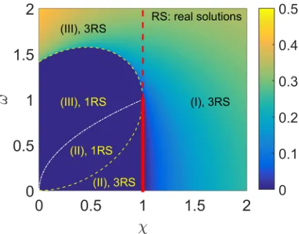
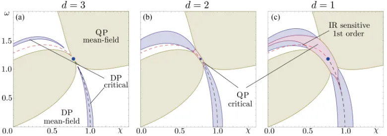
δn =0⇔n˜[
FIG. 2. Scaling regimes for the second-order phase transition in dimensionsd=3,2,1. In the white region, mean field scaling behavior according to classical directed percolation (DP) is observed, while the blue region corresponds to critical scaling of the classical DP universality class below the Ginzburg scale. In the yellow regions, the dynamics is dominated by the mean field behavior of the quantum contact process (QP). The critical behavior of the QP corresponds to the bicritical point and is found in the red region. The black (red) dashed line indicates the line of second- (first-) order transitions. Remarkably, in one dimension, the first-order transition is located partly in the critical regime and experiences strong infrared corrections.
where the primes are the standard notation for differentiation with respect to the argument. A further simplification comes from the properties of the response fields: according to Eq. (2.47),
˜
n= n˜Xξ =
! δ1
δhn X
"
ξ
hn=0
=0, (3.5)
i.e., ˜nis the response of the identity to an external field and therefore trivially vanishes. Hence, one finds the intuitive result that the properties of the system are encoded in the potential (2.53) (reported here for convenience)
(n)=
2n
2+u3
3n
3+u4
4 n
4, (3.6)
with the couplings (2.54)–(2.57). The potentialdescribes the deterministic dynamicsin the absence of noise and spatiotem-poral fluctuations; in the long-time limit, this dynamics will relax towards its global minimum, whose properties thereby determine the thermodynamic phases and the in-between phase boundaries. The corresponding results are reported in the left panel of Fig.1. Recalling thatu4 is always positive,
one can distinguish three different regimes:
(I) For <0, has a single minimum at finite density
nX=nMF= −
u3+ √
u2 3−4u4
2u4 . This region is thus a portion of the active phase.
(II) For >0, u3>0, there is a single minimum of the
potential atnX=0 and the absorbing state is the steady state
of the system.
(III) For parameters >0, u3<0, has one local
minimum atnX=0 and a second local minimum atnX=nMF.
In the absence of noise, the system will always relax towards the global minimum of the potential, which is located at
nX=0 foru3> uc= −3
#
u4
2 and atnX =nMFforu3< uc.
The nature of the transition between the active and the absorbing phases depends on the position in parameter space. We start from the boundary separating (I) from (III), corresponding to the regime dominated by the quantum limit (B) discussed above: foru3 <0, i.e., forω >
√
χ(χ+1)/2,
the phase transition takes place atu3=uc. As the transition
line is crossed, the density jumps from zero to a finite value. Furthermore, the system remains gapped ( >0) at the transition and keeps a finite correlation lengthξ =√D/ <
∞. These are hallmarks of a discontinuous, first-order phase transition. Due to the finite correlation length, the theory remains well behaved at long wavelengths (i.e., free of infrared singularities) and the qualitative mean field picture does not break down once fluctuations are included. The latter will only lead to perturbative corrections of the system parameters, which may become quantitatively substantial, but remain fi-nite. An interesting situation appears in one spatial dimension, where the critical region of the neighboring bicritical point, i.e., the region where critical fluctuations become comparable with the mean field couplings and therefore dominate the behavior of the system, grows to encompass part of the first-order line (see Fig. 2). This leads to strong, infrared-dominated corrections to the dynamics of the first-order transition. An estimation of the extension of the critical region via the calculation of the corresponding Ginzburg scale [99] will be provided further below. Apart from spatial fluctuations, one has to consider the effect of the nonequilibrium noise vertices
. Their effect is nonperturbative and leads to a shift of the transition line, which is discussed in Sec.V.
Foru30, the transition takes place when the gap vanishes (=0), corresponding to the boundary between (I) and (II) and to the regime dominated by classical physics (B). In this case, the density varies continuously across the transition and the phase transition is of second order. Due to the vanishing gap, spatial fluctuations induce infrared-divergent corrections to the dynamics and the mean field picture is significantly modified. The relevant scaling and the corresponding regimes are discussed in Sec.III C.
Finally, a special role is played by the point (,u3)=
(0,0) [lying within (C)] at which the first- and second-order transition lines terminate. This represents a bicritical point, for which the physics is dominated by the coherent vertexu4∼ω2
![Table I or Table 2 in Ref. [24]).](https://thumb-us.123doks.com/thumbv2/123dok_us/8566680.367269/13.608.311.559.366.402/table-i-or-table-in-ref.webp)
![FIG. 4. Optimal path approximation. (a) Phase space (n,optimal path approachtrajectories for parametersdot in parameter space in (b)]](https://thumb-us.123doks.com/thumbv2/123dok_us/8566680.367269/17.608.313.558.71.191/optimal-approximation-phase-space-optimal-approachtrajectories-parametersdot-parameter.webp)