A Bayesian approach to fitting Gibbs processes with temporal random effects

A Bayesian approach to fitting Gibbs processes with

temporal random effects

Ruth King

, Janine B. Illian

, Stuart E. King

, Glenna F.

Nightingale

and Ditte K. Hendrichsen

1

_{School of Mathematics and Statistics, University of St Andrews,}

St Andrews, Fife, Scotland

2

_{Norwegian Institute For Nature Research, N-7047, Trondheim,}

Norway

[email protected]

Abstract

We consider spatial point pattern data that have been observed re-peatedly over a period of time in an inhomogeneous environment. Each spatial point pattern can be regarded as a “snapshot” of the underlying point process at a series of times. Thus, the number of points and cor-responding locations of points differ for each snapshot. Each snapshot can be analysed independently, but in many cases, there may be little information in the data relating to model parameters, particularly pa-rameters relating to the interaction between points. Thus, we develop an integrated approach, simultaneously analysing all snapshots within a single robust and consistent analysis. We assume that sufficient time has passed between observation dates so that the spatial point patterns can be regarded as independent replicates, given spatial covariates. We develop a joint mixed effects Gibbs point process model for the replicates of spa-tial point patterns by considering environmental covariates in the analysis as fixed effects, to model the heterogeneous environment, with a random effect (or hierarchical) component to account for the different observation days for the intensity function. We demonstrate how the model can be fitted within a Bayesian framework using an auxiliary variable approach to deal with the issue of the random effects component. We apply the methods to a dataset of muskoxen herds and demonstrate the increased precision of the parameter estimates when considering all available data within a single integrated analysis.

Keywords: Data augmentation; Markov chain Monte Carlo; Mixed effects model; Muskoxen data; Spatial and temporal point processes

1

Introduction

technically challenging. Recent technology facilitates the collection of spatially explicit data, for example via the use of GPS/Argos collars attached to indi-viduals that record the location of the individual at given time intervals over a period of time until the end of the experiment or the device “fails” (for exam-ple from battery failure or the device becoming detached from the individual). Applications range from large terrestrial (Babin et al. 2011 and Langrock et al. 2012, bison; Morales et al. 2004, elk) and marine mammals (Johnson et al. 2008, harbour seal; Jonsen et al. 2005, McClintock et al. 2012, grey seal) to small insects (Wikelski et al. 2010, orchid bees) to name just a few. In such studies, the biological mechanisms of interest often relate to the movement of individuals over time and attributed to different underlying behaviours (Black-well 2003, Morales et al. 2004, Breed et al. 2009 and McClintock et al. 2012). However, in such studies only very few individuals from the study population are typically monitored and the resulting data for individuals either analysed independently of each other or assuming a common underlying model. Re-cently, multiple animals have been considered simultaneously using hierarchical random effect models to allow for individual variability, yet still only a small proportion of all individuals are typically tagged (Langrock et al. 2012). Con-sequently, it is difficult to directly model interactions between individuals and draw meaningful biological conclusions relating to interactions between different individuals/groups.

Alternatively, using for example an aerial survey, a snapshot can be taken of the locations ofallindividuals within a given study area at a particular point in time, i.e. a spatial pattern formed by the individuals at a given time (Cornulier and Bretagnolle 2006, Illera et al. 2010). However, there is often limited infor-mation contained within a single point pattern for drawing robust conclusions on the ecological mechanisms of interest. This may lead to a series of point pat-terns collected at repeated points in time. The snapshots of the same biological species may be taken over different (non-overlapping) geographical regions or repeatedly over the same study region for mobile individuals (as we will consider in this paper). For such repeated point pattern data, individual points (i.e. in-dividuals) are not uniquely identifiable (i.e. given any two individual points in different snapshots we cannot identify whether they are the same individual or not) so it is not possible to consider explicit spatio-temporal movement models similar to those developed for GPS data, since these require the time-series of the locations of individual animals. Thus, such snapshot data can be seen to be in direct contrast to GPS collar data in that snapshots provide the location of all individuals but only for a small number of times (possibly a single time); whereas GPS collar data typically provides a long time-series of data on only a small number of individuals (possibly only a single individual).

location of their prey, while prey will be repulsed from the location of their predators or animals may exhibit territorial behaviour. Plants may repel each other as they compete for the same available resources, so that plants may be unable to grow near another plant due to limited resources (one of the indi-vidual plants is unable to compete as effectively for the resources and dies). Alternatively, individuals may attract each other through mechanisms such as facilitation where a plant species provides nutrients for another species (Brooker et al. 2008, Illian et al. 2009). Individuals within a plant or animal popula-tion typically perceive only their local neighbours and hence predominantly interact with these (Law et al. 2001). Hence, the parameters in a Gibbs (or Markov) point process model reflect local spatial interactions as well as the underlying intensity of the points. Interactions can be regarded as “negative” or “positive” between points, corresponding to repulsion or attraction among individuals. Heterogeneity within the study area that may influence the local intensity and/or interaction within the pattern, may be modelled via the use of spatial covariate information. If covariate data are available, these are typically included in a Gibbs process model as a fixed effect, often by a parametric func-tion of the given spatial covariate(s) (Baddeley and Turner 2000; Baddeley and Turner 2006).

We consider a series of spatial point pattern data observed over a period of time, rather than a single point pattern. In many applications the number of observed points in a single pattern may be too low for the resulting estimates to be reliable, with very poor precision of the parameter estimates. Alternatively, in other cases, even when it is possible to obtain estimates of the intensity and interaction parameters for each independent dataset it can lead to inconsistent parameter estimates among the different snapshots. This makes it more difficult to sensibly interpret the model parameters, particularly if there is a general interest in population dynamics across years rather than within the specific years. We present an integrated approach where we jointly model all the spatial point patterns within a single analysis.

of different regions) or temporal variability (for repeated snapshots of the same region) within a consistent framework. For the muskoxen data described in Section 2, snapshots are taken on a weekly basis during the study period. To demonstrate the methodology we consider snapshots which correspond to a lag of (approximately) one year, removing any potential dependence between suc-cessive snapshots (conditional on spatial covariates) and the need to consider additional factors such as seasonal migration (see Section 2 for further discus-sion).

We follow Illian and Hendrichsen (2010) who propose a mixed effects model resulting from replicated spatial point patterns, allowing for a temporal random effect component within the model combined with a fixed effects environmental component. In particular, they re-express the conditional likelihood so that it is equivalent to the log-likelihood of independent weighted Poisson variables using the Berman-Turner device. Consequently, this permits the calculation of the MLEs of the parameters via the use of standard software for generalised linear mixed models (GLMMs). However, this model-fitting approach assumes independence among the points of a single snapshot within the log-likelihood expression, so that the standard errors of the parameters and resulting test statistics generated by the software cannot be interpreted directly.

In this paper, we provide a framework for fitting mixed effects models within a Bayesian setting, where we are able to estimate the uncertainty associated with the parameter estimates, for example, using posterior credible intervals. In Section 2 we introduce the data and provide the mathematical notation used throughout. In Section 3 we describe a mixed effects model, where there are both fixed effects, corresponding to the environmental covariate, and temporal random effects that may influence the intensity of the point process. In Section 4 we describe a Bayesian approach (using Markov chain Monte Carlo and data augmentation) that can be used to fit the mixed effect model. We present the corresponding results obtained for the given data in Section 5. Finally, we conclude with a discussion in Section 6.

2

Data and Notation

the autumn rut. Considering snapshots of (approximately) one year apart, it seems reasonable to be able to assume that they are independent of each other, due to the very long time lag between snapshots. In addition, considering the snapshots taken at the same time of year reduces additional temporal variability due to seasonal affects, including seasonal migration. The data snapshots are presented in Figure 1, including the corresponding boundary of the study area, plotted with graded contours for the altitude of the region. Clearly, we can see from the figure that there appears to be substantial variability in the number of muskoxen herds observed in the study period over time, from a minimum of 16 herds in 1999 to a maximum of 54 herds in 2004. In addition, Figure 1 suggests that the location of the herds are negatively related to altitude (i.e. there are fewer herds at higher altitudes), which has been identified in previous analyses (Forchhammer et al. 2008). Thus, we include altitude as an environmental covariate in the analysis.

[Figure 1 about here.]

Notationally, we let Nt denote the number of observed muskoxen at time t = 1, . . . , T, where T = 9, corresponding to years 1999 to 2007 and xtj the

location of herdj= 1, . . . , Ntat timet= 1, . . . , T. For notational convenience,

we letxt={xtj :j= 1, . . . , Nt}, so thatxt denotes the set of muskoxen herd

locations at time t = 1, . . . , T. In other words xt denotes the spatial point

pattern data at timet. The muskoxen herds represented by the points observed at a given time are assumed to interact. However, since the muskoxen herds are motile, they only interact with muskoxen observed at the same time point and are assumed to be independent of muskoxen locations at all other time periods, i.e. xt1 andxt2 are independent for t16=t2 (conditional on the environmental

covariate). Further we setx={xt:t= 1, . . . , T}, so thatxdenotes the set of

all spatial point pattern data. We let W denote the study region. Finally, for locationu∈W, we let y(u) denote the corresponding (normalised) altitude of locationu, and set y ={y(u) : u∈ W}. We note that in this exampleW is constant over time, but more generally it is possible to allow the study region to vary over the time points. Similarly, while the covariate altitude does not vary among the time points it is straightforward to include time-varying covariates in the model.

3

Models

We assume that the point patternsx1, . . . ,xT are independent (conditional on

environmental covariate) and random effects (relating to temporal heterogene-ity).

3.1

Area interaction process

We note that many Gibbs processes, in particular pair-wise interaction pro-cesses, may only be used to model repulsive inter-individual interaction. Ani-mals that display scramble competition, i.e. utilize resources which they do not have exclusive access to, face a degree of cost associated with social interactions over access to forage and other resources, which may lead to such a repulsive interaction (Nicholson 1954; Hassell 1975). However, conversely, several factors may cause animals to aggregate, including kinship, mating behaviour and preda-tor avoidance (Caraco et al. 1980; Janson 1988). Ungulates can exhibit both attraction and repulsion towards each other depending on factors such as the age, sex and breeding status (Li et al. 2012), so that we use an area interaction process (Baddeley and van Lieshout 1995) to potentially consider both positive and negative interactions for the muskoxen herds.

We initially consider a single spatial point patternxt={xt1, . . . , xtNt}. The

conditional intensity is given by,

λ(xtj;xt) =κtγ−

AW,t(xtj)

t ,

where,

AW,t(xtj) =AW,t(xt)− AW,t(xt\{xtj})

such thatAW,t(xt) denotes the area in the region W that lies within distance Rof any of the points inxt={xt1, . . . , xtNt}. Mathematically, if we letD(xtj)

denote the disc of radius R centred at xtj within region W, we can write

AW,t(xt) = ∪Nj=1t D(xtj). Thus, AW,t(xtj) is the area of “single occupancy”

of the discD(xtj) within regionW (i.e. the area of the disc of radiusR centred

atxtj within regionW that does not overlap with any other discs of radius R

centred atxti, for alli6=j).

We follow the approach used in R-library spatstat(Baddeley and Turner 2011) and use the transformation to the canonical scale-free parametrisation by settingηt=γπR

2

t andβt= κ_ηtt. Thus, the conditional intensity can be written

as

λ(xtj;xt) =βtηt1−BW,t(xtj),

whereBW,t(xtj) =AW,t(xtj)/πR2 and 1−BW,t(xtj) can be interpreted as the

proportion of the disc centred atxtj that overlaps with the union of all other

discs centred atxtifori6=j within regionW, or the proportion of the area of

“multiple occupancy” for pointxtj with respect toxt\xtj. The parameter βt

is the intensity of the process and the parameter ηt relates to the interaction

pseudolikelihood is given by,

f(xt|βt, ηt) = α(βt, ηt) Nt Y j=1

λ(xtj;xt)

= α(βt, ηt)βtNtη

(Nt−BW,t(xt))

t , (1)

whereBW,t(xt) =PNj=1t BW,t(xtj). The term α(βt, ηt) is given by,

α(βt, ηt) = exp

−

Z W

λ(u;xt)du

,

such that foru /∈xt,

λ(u;xt) =βtη(1t −BW,t(u)),

whereBW,t(u) =AW,t(u)/πR2= [AW,t(xt∪ {u})− AW,t(xt)]/πR2.

It is possible to fit separate area interaction processes to each dataset xt

independently of the other datasets. However, we now extend these processes to allow for the intensity to be a function of the environmental covariates (in this case using altitude as an example) with a random effects component to model the temporal heterogeneity, allowing information to be shared across the different datasets.

3.2

Mixed effects model

We consider, in turn, the intensity and interaction functions within the model. For the intensity function, we assume a mixed effects model consisting of a fixed effects component relating to the environmental covariate (altitude) and a random effects (or hierarchical) component to model temporal heterogeneity. We initially assume that the interaction function, modelling the interaction among herds, is constant over time and space, but extend to a random effects model for the interaction function in Section 5.

We begin with the (more complex) intensity function. Fort= 1, . . . , T, we specify the intensity function, evaluated at locationu∈W to be of log-linear form,

βt(u) = exp(θ1+φ1,t+δ×y(u)), (2)

so that the intensity parameters are a function of location, and set

φ1,t∼N(0, σ2),

for t = 1, . . . , T. The term θ1 denotes the underlying intensity rate; φ1 =

{φ1,t : t = 1, . . . , T} the temporal random effects on the intensity rate with

random effect variance term, σ2_{, and δthe (homogeneous) fixed effect}

regres-sion coefficient for the environmental covariate. We use normalised values for

We now consider the interaction function. We assume that the interaction strength among the muskoxen herds is constant over time and study area. Thus, we setηt=η for allt= 1, . . . , T, and reparameterise to setθ2= logη. Within

this model a value ofθ2 >0 corresponds to attraction among the herds, while

θ2<0 corresponds to inhibition.

3.3

Likelihood

The model parameters to be estimated are ζ = {θ1, δ, σ2, θ2}. We initially

consider the contribution to the likelihood for a single snapshotxt, extending

equation (1). The intensity parameter is a function of the observed (normalised) environmental covariates y and random effect component. Substituting the interaction and intensity functions into equation (1) and integrating out the random effect termφ1,t, we obtain the likelihood contribution for snapshott,

f(xt|ζ,y) = Z

R



αt(ζ) exp (θ2×[Nt−BW,t(xt)]) Nt Y j=1

exp(θ1+φ1,t+δ×y(xtj))p(φ1,t|σ2)  dφ1,t,

where p(φ1,t|σ2) denotes the probability density function of a N(0, σ2)

distri-bution evaluated atφ1,t and,

αt(ζ) = exp

−

Z W

exp(θ2×[1−BW,t(u)]) exp(θ1+φ1,t+δ×y(u))du

. (3)

We note that the functionBW,t(·) has no closed mathematical form. To evaluate

this function atu, say, we use a Monte Carlo type approach, randomly simu-lating a set of points inD(u), the disc centred atuwithin the region W, and calculate the proportion of points that fall in an area of “multiple occupancy” (i.e. within a distance ofRfrom any point inxt\{u}). The integral within the

function for theαterm is analytically intractable, and is calculated via numer-ical integration. Note that typnumer-ically the Berman-Turner device (Berman and Turner 1992; Baddeley and Turner 2000) is used to perform this numerical inte-gration in the termαt(ζ) due to the simplification of the likelihood expression,

but in general, alternative numerical integration algorithms can be used. We assume that the spatial point patterns for different times are independent conditional on the environmental covariates, so that we can express the joint pseudolikelihood over all snapshots, in the form,

f(x|ζ,y) =

T Y t=1

f(xt|ζ,y).

4

Methods

We consider a Bayesian analysis of the data and initially describe the Markov chain Monte Carlo (MCMC) approach that we implement to obtain a sam-ple from the posterior distribution of the model parameters of interest. To reduce the numerical integration necessary in the evaluation of the likelihood expression, we use a data augmentation approach (Tanner and Wong 1987). In particular we introduce the φ1 terms as auxiliary variables (or parameters) to

be estimated within the Bayesian analysis. We then form the joint posterior distribution over the model parameters,ζ, and auxiliary variables,φ, given by,

π(ζ,φ|x,y)∝f(x|ζ,φ,y)p(ζ,φ).

We briefly discuss the priorp(ζ,φ), before considering the (conditional) likeli-hood termf(x|ζ,φ,y). The prior on the parameters can be decomposed into,

p(ζ,φ) =p(ζ)p(φ|σ2).

Assuming independence of the temporal random effects, we can write,

p(φ|σ2) =

T Y t=1

p(φ1,t|σ2),

where p(φ1,t|σ2) denotes the density of a Normal distribution with mean 0

and varianceσ2_{, corresponding to the temporal random effect component. We}

specify independent priors on the model parameters of the form,

θi∼N(µi, τi) i= 1,2; σ2∼Γ−1_(a

1, a2); δ∼N(µδ, τδ).

With no expert prior information on these parameters, we setµ1=µ2=µδ = 0; τ1 =τ2 =τδ = 1002 and a1=a2 = 0.001. Note that we perform a prior

sen-sitivity analysis by considering different prior specifications on the parameters (see Section 5 for further discussion).

We now return to consider the termf(x|ζ,φ₁,y), which can be regarded as the conditional pseudolikelihood of the data, given both the model parameters,

ζ, and random effect terms, φ1. This (conditional) pseudolikelihood can be

explicitly written as,

f(x|ζ,φ1,y) = T Y t=1

ft(xt|ζ,φ1,y),

where

ft(xt|ζ,φ1,y) =αt(ζ) exp (θ2×[Nt−BW,t(xt)]) Nt Y j=1

whereαt(ζ) is given in equation (3). The posterior distribution of the model

pa-rameters,ζ, can then be obtained by taking the marginal posterior distribution (i.e. integrating out over the random effects terms,φ₁),

π(ζ|x,y) =

Z

π(ζ,φ1|x,y)dφ1.

Thus, the Bayesian approach does not remove the necessity of integrating out the random effect terms, but the integration is essentially performed within the MCMC algorithm, which obtains a sample from the joint posterior distribution over both ζ and φ. Given a sample from the joint posterior distribution, to obtain a sample from the marginal distribution of ζ (i.e. to integrate out over

φ), we simply take the sampledζvalues, irrespective of the associated values of

φand calculate the corresponding summary statistics of interest (as we would when simply calculating marginal posterior summary statistics of a single pa-rameter in any Bayesian analysis). See King et al. (2009) and Bonner et al. (2010) for further discussion.

To obtain a sample from the joint posterior distributionπ(ζ,φ|x,y) we use a hybrid or Metropolis-within-Gibbs algorithm. In particular, at each iteration of the Markov chain, we cycle through each parameter and update the parame-ter using either a random walk Metropolis-Hastings step with Normal proposal density or Gibbs step (if the posterior conditional distribution is of standard form), see for example Brooks (1998) for further details. In particular, we use a Gibbs step forσ2_{(since the posterior conditional distribution has an Inverse}

Gamma distribution) and a Metropolis-Hastings step for all other parameters. To obtain efficient proposal updates for the Metropolis-Hastings step we used a pilot-tuning procedure that involved running a series of short MCMC simula-tions using a variety of different Normal proposal variances and comparing the mixing of the subsequent chains via a combination of trace plots, mean accep-tance probabilities and autocorrelation function (acf) plots. To obtain a sample from the marginal distributionπ(ζ,σ2|x,y), we simply consider only those re-alisations from the MCMC algorithm for the model parametersζ (essentially integrating out over the random effect terms). However, we note that using this approach we are also able to immediately provide posterior marginal estimates of the random effect parameters, which may be of interest themselves, as they provide information on the magnitude and/or sign of the random effect at each time.

5

Results

We initially analyse each individual spatial point pattern separately. We then consider an integrated analysis, simultaneously analysing all available data, us-ing random effects to model temporal heterogeneity, providus-ing a consistent and robust approach. We set an interaction radius for the discs centred on each point to beR= 125. This is slightly larger than the interaction radius used by Illian and Hendrichsen (2010), who use 2R= 200 and consider a pairwise inter-action function. The specification of the slightly larger radius here is to ensure there are observed overlaps between at least two herds within each dataset.

5.1

Independent analysis

We analyse each spatial point pattern independently for each year from 1999 to 2007, so that we have parameters θ1,t, θ2,t andδt for t= 1, . . . ,9. The

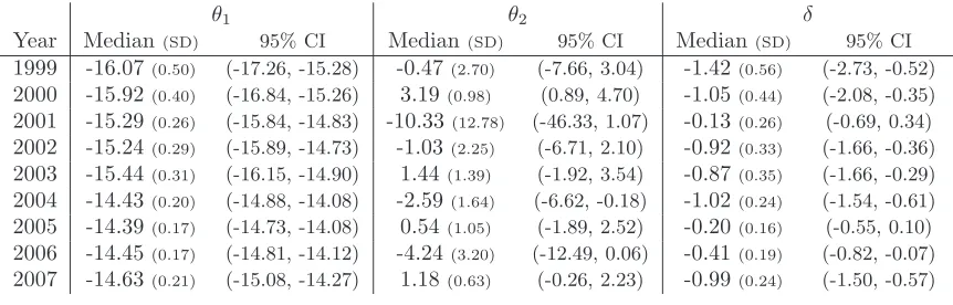
corre-sponding MLEs are presented in Table 1(a) and the posterior median (standard deviation) and 95% symmetric credible interval (CI) using the Bayesian analysis in Table 1(b). We use the posterior median as the marginal posterior distribu-tions for the interaction parameter θ2 is skewed in a number of years. The

posterior medians appear to be generally similar to the corresponding MLEs of the parameters (differences are greatest for the most heavily skewed posterior marginal distributions). Clearly, there appears to be significant variability in es-timates of the intensity parameterθ1,t over time (with several non-overlapping

credible intervals between years). The posterior estimates of the interaction parametersθ2,thave relatively low precision (high posterior standard deviation

and wide 95% symmetric CIs), suggesting that, in general, there is limited infor-mation in a single spatial point pattern to estimate the interaction parameter. However, there is possibly some evidence that the interaction also varies over time, with some non-overlapping credible intervals with regard toθ2,t, and the

value of 0 not contained within three 95% symmetric CIs (corresponding to no interaction present). The regression coefficient δ appears to be fairly similar across years, allowing for the uncertainty with regard to the estimate. For ex-ample, the 95% symmetric CIs for δ all overlap for the different years. The years with smaller numbers of herds observed (1999-2003, with a range of 16-25 herds) have generally wider credible intervals on the parameter estimates than years where larger numbers of herds are observed (2004-2007, with a range of 40-54 herds). This is to be expected, since the larger the number of data points observed within a single snapshot, the greater the amount of information in the dataset regarding the parameters. One would normally not attempt to fit a model to patterns as small as those for the earlier years, as there is not enough information in the data of a single pattern for inference.

[Table 1 about here.]

within the model described in Section 3 we initially assume the same interaction function and spatial environmental covariate dependence (i.e.θ2andδ) for each

dataset, but allow for additional temporal variability in the intensity function via the additional random effects component, as described in Section 3.2.

5.2

Integrated analyses

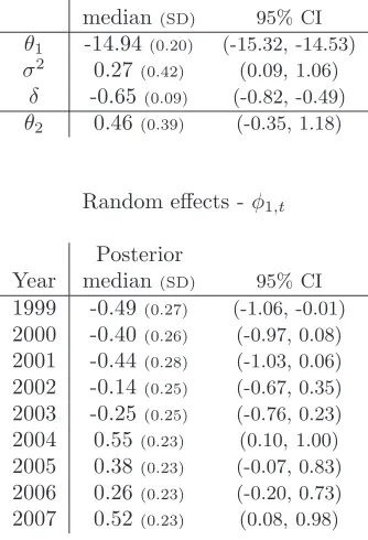
We initially consider a mixed effects model for the intensity function and fixed effects (time homogeneous) model for the interaction function. The correspond-ing posterior summary statistics for the parameters are provided in Table 2. Clearly, the environmental covariate (altitude) has a negative influence on the intensity of the spatial point pattern (posterior probability of 1.00 that the in-fluence is negative). In addition, there appears to be a fairly strong temporal effect on the underlying intensity rate of the spatial point patterns, with a poste-rior median of 0.27 for the random effect variance and 95% symmetric CI (0.09, 1.06). The random effect terms φfor the intensity function can be estimated directly, as they are imputed within the MCMC simulations. Given the presence of a temporal random effect, there is positive evidence (Bayes factor >3) for a negative temporal random effect compared to the underlying mean intensity rate in 2003 and strong evidence (Bayes factor>20) in years 1999-2001 (Kass and Raftery 1995). Similarly, there is positive evidence of a positive temporal random effect in 2005 and 2006, and strong evidence in years 2004 and 2007. The posterior probability of a positive interaction (i.e. θ2>0) is equal to 0.87

(or Bayes factor of 6.8) providing positive evidence of clustering of the herds.

[Table 2 about here.]

These results appear to reflect the increase in population size between 1999 and 2007 reported by Hansen et al. (2011). During this period the population density in the valley (measured as the maximum number of animals observed from a fixed point on any given day during the summer census) increased from (approximately) 20 individuals in 1999 to 110 in 2007, after which it has started to decrease again (Hansen et al. 2011). The population in the Zackenberg region is part of a larger population spanning Wollaston Foreland, Clavering Island and adjacent regions, so that the population increase does not reflect changes in population size per se, but the net influx of animals into the Zackenberg valley during the summer season. This influx is likely to be caused by a higher than average forage availability and/or quality (Forchhammer et al. 2005), an assumption supported by the seasonal increase in calves, yearlings and females (Berg 2003; Hansen et al. 2011), i.e. animals with need for high quality forage. Comparing the integrated results with those obtained from the separate anal-yses in Table 1, we can clearly see that the posterior precision of the parameters (θ1, δ andθ2) is significantly improved within the integrated analysis. This is a

negative effect of altitude on intensity (i.e. fewer herds at higher altitudes). In the single analyses for each year, there is greater uncertainty in the magnitude of the effect of altitude on the intensity and even the sign of this parameter in years 2001 and 2005. In addition, within the independent analyses, the sign of the interaction parameter, θ2, corresponding to attraction/repulsion is

gener-ally unclear. However, within the integrated analysis, there is positive evidence that the interaction is positive, corresponding to clustering of muskoxen herds which is likely to be related to the spatial distribution of food resources causing herds to aggregate in areas with access to forage. In particular, there is con-siderable variation in the distribution of plant communities within the census area (Elberling et al. 2008) and muskoxen show a clear preference for vege-tation areas dominated by fen, grassland and salix snow beds, accounting for approximately 75 percent of observations, although these vegetation types only represent approximately 30 percent of the census area (Berg et al. 2008).

5.3

Sensitivity Analyses

We consider the sensitivity of the results on both the priors specified on the parameters and the modelling assumptions. We begin by considering the sensi-tivity of the posterior results on the priors specified. In particular, we increase the prior standard deviation of the Normal priors on the underlying intensity rate, θ1, and interaction parameters, θ2, by a factor of 10 and also specify

σ∼U[0,100] (Gelman 2006). The posterior results appear to be insensitive to these different priors, with the same interpretation of the posterior results.

To assess the sensitivity of the model assumptions we consider a range of sensitivity analyses. In particular, we consider (i) the model with an additional temporal random component in the interaction function; (ii) changing the spec-ified interaction radius; and (iii) removing the independence assumption on the random effect terms for the intensity function. We consider each in turn.

(i) Temporal random effects for interaction function

We consider an additional temporal random effect component on the interaction parameter, analogous to the random effect component on the intensity param-eter. In particular, for the observed point processxt fort= 1, . . . , T, we set,

ηt= exp(θ2+φ2,t),

such that φ2,t ∼ N(0, ν2), independently, and where ν2 is a parameter to be

estimated. The corresponding likelihood contribution for point process xt is

given by,

f(xt|ζ, ν2,y) = Z

R

Z

R



α(ζ_t, ν2_{) exp ([θ}

2+φ2,t]×[1−BW,t(xt)])

×

Nt Y j=1

exp(θ1+φ1,t+δ×y(xtj))p(φ1,t|σ2)p(φ2,t|ν2) 

where p(·|·) denotes the probability density function of a normal distribution with mean zero and given variance term, evaluated at the specified value, and

α(ζ_t, ν2) = exp

−

Z W

exp([θ2+φ2,t]×[1−BW,t(u)]) exp(θ1+φ1,t+δ×y(u))du

.

A data augmentation approach, analogous to that described in Section 4 can be implemented, introducingφ2 = {φ2,t :t = 1, . . . , T} as auxiliary variables

within the Bayesian analysis.

The results obtained for the underlying intensity rate and regression coeffi-cient were generally very similar, with only minor changes in the posterior sum-mary statistics for these parameters. For example, the posterior median (95% symmetric CI) for θ1 and δ were −14.94 (−15.31, −14.51) and−0.64 (−0.81,

−0.48), respectively. The estimates of the intensity random effect terms (σ2_and

φ₁) were generally similar (posterior median (95% CI) forσ2_{of 0.29 (0.10, 1.24)}

- the credible interval is slightly larger than for the previous model, which is to be expected since an additional parameter has to be estimated). In particular the interpretation of the random effect terms on the intensity parameters re-mains consistent, with evidence for a negative random effect in years 1999-2001 and 2003 and a positive random effect in years 2004-7. The underlying inter-action parameter θ2 has a significantly increased posterior standard deviation

with the addition of temporal heterogeneity on the interaction function. The posterior median (standard deviation) of 0.09 (0.98) and 95% CI(-2.24, 1.81). The corresponding random effect variance has posterior median (95% symmetric CI) of 3.31 (0.31, 20.73). There is only (positive) evidence for three years that the interaction differs to the mean underlying interaction rate, corresponding to a higher interaction in 2007 and lower interaction in years 2004 and 2006. This sensitivity analysis suggests that there is relatively little information contained in the data relating to the interaction among the muskoxen herds, leading to a generally poor precision of the estimation of these parameters.

(ii) Interaction radius

(−3.83,−0.19), with fewer points within the interacting distance of each other. When the interaction radius in increased, there is evidence for a clustering effect (posterior median of θ2 of 1.33 with 95% symmetric CI (0.80, 1.82) due

to the number of points within the interacting distance of each other. However, in all analyses, the negative relationship between the intensity and altitude is consistent, with posterior medians forδ within ±0.03 of the previous analysis with R = 125 and very similar widths for the 95% credible intervals. The underlying mean intensity rate, θ1, is consistent for the different interaction

radii, with the same posterior median to 1 decimal place, and similar width 95% credible intervals; and the same years identified (2004 and 2007) with the 95% symmetric CIs for the random effects terms not containing 0 within the intensity function.

(iii) Dependent temporal random effects

Finally, we remove the independence assumption on the random effect error terms and consider alternative (non-independent) random effect models: a ran-dom walk and a moving average of order 1 (i.e. anM A(1) model). For example, the random walk process is specified such that fort= 2, . . . , T,

φ1,t∼N(φ1,t−1, σ2RW)

where σ2

RW is the associated random walk variance to be estimated. For the M A(1) model fort= 2, . . . , T, we specify,

φ1,t=kωt−1+ωt,

such thatωs∼N(0, σM A2 ), independently for alls= 1, . . . , T. For identifiability

for both models we specifyφ1,1= 0. We specify independent (non-informative)

priors, such that σ2

RW, σM A2 ∼ Γ−1(0.001,0.001) and k ∼ N(0,1002) for the AR(1) andM A(1) models.

For each of these models, very similar results are obtained for the environ-mental regression coefficient,δ, intensity parameters for each year, (θ1+φ1,t)

fort= 1, . . . , T and interaction parameter,θ2 (i.e. the same posterior median

and 95% CIs to 2 significant figures). For the M A(1) process, the posterior median (95% CI) forσ2M Ais 0.17 (0.05, 0.71), and fork, 0.37 (-0.18, 0.82). The

posterior credible interval for the variance component significantly overlaps with that obtained assuming independent random effects (see Table 2). In particular, the probability that the random effect variance for the M A(1) model is lower than that for the independent model,Pπ(σM A2 < σ2), is 0.68 (or Bayes factor of

2.16), which does not provide positive support for a lower variance component. In addition, the value of k = 0, corresponding to independent random effects is also contained within the 95% CI for this parameter. For the random walk the posterior median (95% CI) for the random effect variance component,σ2

RW,

probability that the variance component is less for the random walk model than the independent model,Pπ(σRW2 < σ2), is 0.73 (or Bayes factor of 2.81), close

to positive evidence of a smaller variance term (Kass and Raftery 1995). How-ever, we note that with only 9 snapshots within our data series, the ability to identifying additional structure within the random effects will be limited.

Overall, the similarity in the results and corresponding interpretation for the intensity and regression coefficient parameters across the different models and priors suggests that these results are generally robust with regard to the model specified on the interaction function.

6

Discussion

Collecting ecological data on population dynamics and spatial distribution of long lived animals is associated with a number of logistic and often also fi-nancial challenges. Data series following a certain population of individually marked animals over long time whilst sampling a wide range of biotic and abi-otic parameters, such as the Soya sheep data from St Kilda (Clutton-Brock and Pemberton 2004) are of high value in ecology, but uncommon. Fragmented and/or sparse data sets are common in biology, and may pose a limit to the ecological questions that can be addressed. Nevertheless, understanding the temporal and/or spatial dynamics of populations is of fundamental importance for species management and conservation (Aarts et al. 2008). The spatial po-sition of animals is of paramount importance in understanding the interactions of individuals, populations and species with their environment. Methods which can aid transferring of data from data-poor to data-rich areas or utilise repeated measures more efficiently are therefore potentially relevant within a wide range of biological applications.

parameter for the study dataset. Using this approach for the muskoxen data there appears to be evidence for a strong negative relationship between the in-tensity of the muskoxen and the altitude, so that muskoxen appear to prefer the lower regions of the study area, previously identified by Forchhammer et al. (2005). This relationship is less clear within the single independent analyses. For the given dataset, we primarily considered a random effect component on the underlying intensity parameter, but the approach is generalisable, for ex-ample, to allow for temporal heterogeneity on the regression coefficient for the environmental covariate. Since interaction concerns second and higher order information in the data there is typically less information contained within the data relating to the interaction function than the intensity function. In partic-ular in the context of datasets with relatively few observed points, this would also suggest that it may be difficult to identify temporal heterogeneity within the interaction parameter, as is the case here when a random effect component was added.

We have described and implemented a Bayesian data augmentation ap-proach, whereby the temporal random effect terms are imputed within the MCMC algorithm and essentially integrated out by considering the marginal distribution of the model parameters. Consequently, since the random effect terms are imputed at each iteration of the Markov chain, obtaining posterior estimates or these random effect terms is immediate. These can be of interest in themselves, for example, in identifying which datasets have a positive/negative temporal random effect component within the intensity function and/or com-paring the magnitude of the random effects between datasets to investigate the strongest deviation from the underlying mean. In addition, and in contrast to the previous approach proposed by Illian and Hendrichsen (2010), we are able to easily obtain posterior credible intervals for each of the parameters providing a measure of the precision of the parameters of interest.

and consequently the specification of biologically plausible priors. Applying such an approach would permit a detailed analyses of the joint factors of social interactions and resource availability which both shape animal spatial distri-butions. Such analyses therefore may provide an improved use of sparse data to explain ecological patterns. In addition, much recent research has focused on developing computationally efficient methods for fitting spatial models in a Bayesian context based on integrated nested Laplace approximations (INLA) (Rue et al. 2009); see also the work by Lindgren et al. (2011). For example, a log Gaussian Cox process model has been fitted to replicated patterns formed by the muskoxen herds (Illian et al 2012a,b), although this approach cannot account for second or higher order spatial behaviour. The application of the INLA approach to such spatial point processes is an area of ongoing research.

Acknowledgements

We would like to thank the Zackenberg Basic programmes who collected the muskoxen data and made the data available to us, with particular thanks to Niels Martin Schmidt. In addition we would like to thank Brett McClintock and Roland Langrock for some useful conversations. The authors also gratefully acknowledge the financial support of Research Councils UK for Illian.

References

Aarts, G., MacKenzie, M., McConnell, B., Fedak, M. and Matthiopoulos, J. (2008), Estimating space-use and habitat preference from wildlife teleme-try data.Ecography 31, 140-160

Babin, J. -S., Fortin, D., Wilmshurst, J. F. and Fortin, M. -E. (2011), En-ergy gains predict the distribution of plains bison across populations and ecosystems.Ecology 92, 240–252

Baddeley, A. J. and Turner, T. R. (2000), Practical maximum pseudolike-lihood for spatial point patterns (with discussion). Australian and New Zealand Journal of Statistics 32, 283–322

Baddeley, A. J. and Turner, T. R. (2006), Modelling spatial point patterns in

R. In A. Baddeley, P. Gregori, J. Mateu, R. Stoica, and D. Stoyan, (eds.),

Case Studies in Spatial Point Pattern Modelling, number 185 in Lecture Notes in Statistics, 23–74. Springer-Verlag, New York

Baddeley, A. J. and Turner, T. R. (2011), spatstat website. URL:

www.spatstat.org.

Berg, T. B, Schmidt, N. M., Høye, T. T., Aastrup, P., Hendrichsen, D. K., Forchhammer, M. C. and Klein, D. R. (2008), High-arctic plant-herbivore interactions under climate influence.Advances in Ecological Research 40, 275–298

Berman, M. and Turner, M. R. (1992), Approximation point process likeli-hoods with GLIM.Journal of the Royal Statistical Society, Series C 41, 31–38

Besbeas, P., Borysiewicz, R. S. and Morgan, B. J. T. (2008), Completing the ecological jigsaw. In D. L. Thomson, E. G. Cooch and M. J. Conroy (eds.),Modeling Demographic Processes in Marked Populations, Springer – Series: Environmental and Ecological Statistics, Volume 3, pp. 513–540 Besag, J. (1978), Some methods of statistical analysis for spatial data.Bulletin

of the International Statistical Institute 47, 77–92.

Besbeas, P., Lebreton, J. D. and Morgan, B. J. T. (2003), The efficient inte-gration of abundance and demographic data.Journal of the Royal Statis-tical Society, Series C 52, 95–102

Blackwell, P. G. (2003), Bayesian inference for Markov processes with diffu-sion and discrete components.Biometrika 90, 613–627

Bonner, S. J., Morgan, B. J. T. and King, R. (2010), Continuous covariates in mark-recapture-recovery analysis: A comparison of methods.Biometrics 66, 1256–1265

Breed, G. A., Jonsen, I. D., Myers, W. D., Bowen, W. D. and Leonard, M. L. (2009), Sex-specific, seasonal foraging tactics of adult grey seals (Halichoerus grypus) revealed by state-space analysis.Ecology 90, 3209– 3221

Brooks, S. P. (1998), Markov chain Monte Carlo method and its application.

The Statistician 47, 69–100

Brooks, S. P. and Gelman, A. (1998), Alternative methods for monitoring con-vergence of iterative simulations.Journal of Computational and Graphical Statistics 7, 434–455

Brooks, S. P., King, R. and Morgan, B. J. T. (2004), A Bayesian approach to combining animal abundance and demographic data.Animal Biodiversity and Conservation 27, 515–529

Brooker, R. W., Maestre, F. T., Callaway, R. M., Lortie, C. L., Cavieres, L. A., Kunstler, G., Liancourt, P., Tielborger, K., Travis, J. M. J., Anthelme, F., Armas, C., Coll, L., Corcket, E., Delzon, S., Forey, E., Kikvidze, Z., Olofsson, J., Pugnaire, F., Quiroz, Q. L., Saccone, P., Schif-fers, K., Seifan, M., Touzard, B. and Michalet, R. (2008), Facilitation in plant communities: the past, the present, and the future. Journal of Ecology 96, 18–34

Cave, V. M., King, R. and Freeman, S. N. (2010), An integrated popula-tion model from constant effort bird-ringing data.Journal of Agricultural, Biological, and Environmental Statistics 15, 119–137

Clutton-Brock, T. H. and Pemberton J. (2004),Soay Sheep, Cambridge Uni-versity Press.

Cornulier T. and Bretagnolle V. (2006), Assessing the influence of environ-mental heterogeneity on bird spacing patterns: a case study with two raptors.Ecography 29, 240–250

Elberling, B., Tamstorf, M. P., Michelsen, A., Arndal, M. F., Sigsgaard, C., Il-leris, L., Bay, C., Hansen, B. U., Christensen, T. R., Hansen, E. S., Jakob-sen, B. H. and Beyens, L. (2008), Soil and plant community-characteristics and dynamics at Zackenberg.Advances in Ecological Research40, 223–248 Forchhammer, M. C., Post, E., Berg, T. B., Høye, T. T. and Schmidt, N. M. (2005), Local-scale and short-term herbivore-plant spatial dynamics reflect influences of large-scale climate.Ecology 86, 2644-2651

Forchhammer, M. C., Schmidt, N. M., Høye, T. T., Berg, T. B., Hendrichsen, D. K. and Post, E. (2008), Population dynamical responses to climate change.Advances in Ecological Research 40, 391–419

Gauthier, G., Besbeas, P., Lebreton, J. D. and Morgan, B. J. T. (2007), Pop-ulation growth in greater snow geese: a modeling approach to integrating demographic and population survey information.Ecology 88, 1420–1429 Gelman, A. (2006), Prior distributions for variance parameters in hierarchical

models.Bayesian Analysis 1, 515–534

Green, P. J. (1995), Reversible jump Markov chain Monte Carlo computation and Bayesian model determination.Biometrika 82, 711–732

Hansen J., Hansen, L. H., Christoffersen, K. S., Albert, K. R., Skovgaard, M. S., Bay, C., Kristensen, D. K., Berg, T. B., Lund, M., Boulanger-Lapointe, N., Sørensen, P. L., Christensen, M. U. and Schmidt, N. M. (2011), Zackenberg Basic: The BioBasis programme. In Jensen, L. M. and Rasch, M. (eds.),Zackenberg Ecological Research Operations, 16th Annual Report, 2010. Aarhus University, DCE Danish Centre for Environment and Energy, 2011. pp. 43–66

Hassell, M. P. (1975), Density-dependence in single-species populations. Jour-nal of Animal Ecology 44, 283-295

Illera, J. C., von Wehrden, H. and Wehner, J. (2010). Nest site selection and the effects of land use in a multi-scale approach on the distribution of a passerine in an island arid environment. Journal of Arid Environments 74, 1408–1412

Illian, J. B., Møller, J. and Waagepetersen, R. P. (2009). Hierarchical spa-tial point process analysis for a plant community with high biodiversity.

Environmental and Ecological Statistics 16, 389–405

Illian, J. B., Penttinen, A., Stoyan, H. and Stoyan, D. (2008). Statistical Analysis and Modelling of Spatial Point Patterns. John Wiley and Sons, Chichester

Illian, J. B., Sørbye, S. H. and Rue, H. (2012a). A toolbox for fitting com-plex spatial point process models using integrated Laplace transformation (INLA).Annals of Applied Statistics– in press

Illian, J. B., Sørbye, S. H., Rue, H. and Hendrichsen, D. (2012b). Using INLA to fit a complex point process model with temporally varying effects – a Case studyJournal of Enviromental Statistics – in press

Janson, C. H. (1988), Food competition in brown capuchin monkeys (Cebus apella): quantitative effects of group size and tree productivity.Behaviour 105, 53-76

Jetz, W., Carbone, C., Fulford, J. and Brown, J. H. (2004), The Scaling of Animal Space Use.Science 306266–268

Jonsen, I. D., Flemming, J. M. and Myers, R. A. (2005), Robust state-space modeling of animal movement data.Ecology 86, 2874–2880

Johnson, D. S., London, J. M., Lea M. -A. and Durban, J. W. (2008), Continuous-time correlated random walk model for animal telemetry data.

Ecology 89, 1208–1215

Kass, R. E. and Raftery, A. E. (1995), Bayes factors.Journal of the American Statistical Association 90, 773–793

King, R., Brooks, S. P., Mazzetta, C., Freeman, S. N. and Morgan, B. J. T. (2008), Identifying and diagnosing population declines: A Bayesian as-sessment of lapwings in the UK.Journal of the Royal Statistical Society, Series C 57, 609–632

King, R., Morgan, B. J. T., Gimenez, O. and Brooks, S. P. (2009),Bayesian Analysis for Population Ecology. CRC Press, Boca Raton

Langrock, R., King, R., Matthiopulos, J., Thomas, L., Fortin, D. and Morales, J. M. (2012), Flexible and practical modeling of animal telemetry data: hidden Markov models and extensions. Under revision for Ecology (Sta-tistical Reports)

Law, R., Purves, D., Murrell, D., and Dieckmann, U. (2001). Causes and effects of small scale spatial structure in plant populations. In J. Silvertown and J. Antonovics (Eds.), Integrating Ecology and Evolution in a spatial context, Blackwell Science, Oxford, pp. 21–44

Lindgren, F., Lindstr¨om, J. and Rue, H. (2011) An explicit link between Gaussian fields and Gaussian Markov random fields: the stochastic par-tial differenpar-tial equation approach (with discussion).Journal of the Royal Statistical Society, Series B 73, 423–498

McClintock, B. T., King, R., Thomas, L., Matthiopulos, J., McConnell, B. J. and Morales, J. M. (2012) A general discrete-time modeling framework for animal movement using multi-state random walks.Ecological Monographs

in press

McCrea, R. S., Morgan, B. J. T., Gimenez, O., Besbeas, P., Lebreton, J. D. and Bregnballe, T. (2010), Multi-site integrated population modelling.

Journal of Agricultural, Biological, and Environmental Statistics 15, 539– 538

Møller, J. and Waagepetersen, R. P. (2007), Modern statistics for spatial point processes (with discussion).Scandinavian Journal of Statistics 34, 643–711

Morales, J. M., Haydon, D. T., Frair J., Holsinger, K. E. and Fryxell, J. M. (2004), Extracting more out of relocation data: building movement models as mixtures of random walks.Ecology 89, 2436–2445

Nicholson, A. J. (1954), An outline of the dynamics of animal populations.

Austalian Journal of Zoology 2, 9-65

Reynolds, T. J., King, R., Harwood, J., Frederikesen, M., Harris, M. P. and Wanless, S. (2009), Integrated data analyses in the presence of emigra-tion and tag-loss.Journal of Agricultural, Biological, and Environmental Statistics 14, 411–431

Rue, H., Martino, S., and Chopin, N. (2009), Approximate Bayesian inference for latent Gaussian models using integrated nested Laplace approxima-tions (with discussion).Journal of the Royal Statistical Society, Series B 71, 319–392

Schaub, M., Gimenez, O., Sierro, S., and Arlettaz, R. (2007), Assessing popu-lation dynamics from limited data with integrated modeling: life history of the endangered greater horseshoe bat.Conservation Biology 21, 945–955. Stoyan, D., Kendall, W. and Mecke, J. (1995), Stochastic Geometry and its

Applications (2nd edn). John Wiley and Sons, London

Tanner, M. A. and Wong, W. H. (1987), The calculation of posterior distri-bution by data augmentation.Journal of the American Statistical Asso-ciation 82, 528–540

van Lieshout, M. N. M. (2000), Markov Point Processes and their Applica-tions. Imperial College Press, London

Figure 1: The location of the muskoxen in each snapshot for years 1999-2007 and corresponding contours of the altitude, with the boundary of the study area included. 0 200 400 600 800 1000

512 514 516 518 8262 8264 8266 8268 8270 8272 × 1 0 0 0 ×1000 1999 (a) 0 200 400 600 800 1000

512 514 516 518 8262 8264 8266 8268 8270 8272 × 1 0 0 0 ×1000 2000 (b) 0 200 400 600 800 1000

512 514 516 518 8262 8264 8266 8268 8270 8272 × 1 0 0 0 ×1000 2001 (c) 0 200 400 600 800 1000

512 514 516 518 8262 8264 8266 8268 8270 8272 × 1 0 0 0 ×1000 2002 (d) 0 200 400 600 800 1000

512 514 516 518 8262 8264 8266 8268 8270 8272 × 1 0 0 0 ×1000 2003 (e) 0 200 400 600 800 1000

512 514 516 518 8262 8264 8266 8268 8270 8272 × 1 0 0 0 ×1000 2004 (f) 0 200 400 600 800 1000

512 514 516 518 8262 8264 8266 8268 8270 8272 × 1 0 0 0 ×1000 2005 (g) 0 200 400 600 800 1000

512 514 516 518 8262 8264 8266 8268 8270 8272 × 1 0 0 0 ×1000 2006 (h) 0 200 400 600 800 1000

Table 1: Independent analyses for each spatial point pattern for years 1999-2007, using both classical and Bayesian approaches.

(a) MLE for each parameter

θ1,t θ2,t δt

Year MLE MLE MLE 1999 -15.93 0.29 -1.31 2000 -15.81 3.29 -0.98 2001 -15.24 -5.06 -0.11 2002 -15.19 -0.53 -0.89 2003 -15.37 1.60 -0.82 2004 -14.40 -2.38 -1.00 2005 -14.37 0.69 -0.19 2006 -14.43 -3.37 -0.41 2007 -14.60 1.20 -0.97

(b) Posterior median (standard deviation) and 95% symmetric credible interval (CI) for each parameter

θ1 θ2 δ

Year Median(SD) 95% CI Median(SD) 95% CI Median(SD) 95% CI

1999 -16.07(0.50) (-17.26, -15.28) -0.47(2.70) (-7.66, 3.04) -1.42(0.56) (-2.73, -0.52)

2000 -15.92(0.40) (-16.84, -15.26) 3.19(0.98) (0.89, 4.70) -1.05(0.44) (-2.08, -0.35)

2001 -15.29(0.26) (-15.84, -14.83) -10.33(12.78) (-46.33, 1.07) -0.13(0.26) (-0.69, 0.34)

2002 -15.24(0.29) (-15.89, -14.73) -1.03(2.25) (-6.71, 2.10) -0.92(0.33) (-1.66, -0.36)

2003 -15.44(0.31) (-16.15, -14.90) 1.44(1.39) (-1.92, 3.54) -0.87(0.35) (-1.66, -0.29)

2004 -14.43(0.20) (-14.88, -14.08) -2.59(1.64) (-6.62, -0.18) -1.02(0.24) (-1.54, -0.61)

2005 -14.39(0.17) (-14.73, -14.08) 0.54(1.05) (-1.89, 2.52) -0.20(0.16) (-0.55, 0.10)

2006 -14.45(0.17) (-14.81, -14.12) -4.24(3.20) (-12.49, 0.06) -0.41(0.19) (-0.82, -0.07)

Table 2: Posterior median (standard deviation) and 95% symmetric credible interval (CI) for each parameter in the integrated analysis.

Posterior

median(SD) 95% CI

θ1 -14.94(0.20) (-15.32, -14.53)

σ2 _0.27

(0.42) (0.09, 1.06)

δ -0.65(0.09) (-0.82, -0.49)

θ2 0.46(0.39) (-0.35, 1.18)

Random effects -φ1,t

Posterior

Year median(SD) 95% CI

1999 -0.49(0.27) (-1.06, -0.01)

2000 -0.40(0.26) (-0.97, 0.08)

2001 -0.44(0.28) (-1.03, 0.06)

2002 -0.14(0.25) (-0.67, 0.35)

2003 -0.25(0.25) (-0.76, 0.23)

2004 0.55(0.23) (0.10, 1.00)

2005 0.38(0.23) (-0.07, 0.83)

2006 0.26(0.23) (-0.20, 0.73)