Optimizing the mix design of cold bitumen emulsion mixtures using response surface methodology

1

Optimizing the mix design of cold bitumen emulsion mixtures using

response surface methodology.

Ahmed I. Nassar*, Nicholas Thom, Tony Parry.

Nottingham Transportation Engineering Centre, Department of Civil Engineering, Faculty of Engineering, University of Nottingham, University Park, Nottingham NG7 2RD, UK

2

Abstract

Cold mix asphalt (CMA) has been increasingly recognized as an important alternative worldwide. One of the common types of CMA is cold bitumen emulsion mixture (CBEM). In the present study, the optimization of CBEM has been investigated, to determine optimum proportions to gain suitable levels of both mechanical and volumetric properties. A central composite design (CCD) with response surface methodology (RSM) was applied to optimize the mix design parameters, namely bitumen emulsion content (BEC), pre-wetting water content (PWC) and curing temperature (CT). This work aimed to investigate the interaction effect between these parameters on the mechanical and volumetric properties of CBEMs. The indirect tensile stiffness modulus (ITSM) and indirect tensile strength (ITS) tests were performed to obtain the mechanical response while air voids and dry density were measured to obtain volumetric responses.

The results indicate that the interaction of BEC, PWC and CT influences the mechanical properties of CBEM. However, the PWC tended to influence the volumetric properties more significantly than BEC. The individual effects of BEC and PWC are important, rather than simply total fluid content which is used in conventional mix design method. Also, the results show only limited variation in optimum mix design proportions (BEC and PWC) over a range of CT from 10oC to 30oC. The variation range for optimum BEC was 0.42% and 0.20% for PWC. Furthermore, the experimental results for the optimum mix design were corresponded well with model predictions. It was concluded that optimization using RSM is an effective approach for mix design of CBEMs.

3

1. Introduction

Several benefits are gained from using cold mix asphalt (CMA) instead of hot mix asphalt (HMA). The benefits include conservation of materials and energy, preservation of the environment and reduction in cost [1, 2]. One of the common types of CAM is cold bitumen emulsion mixture (CBEM). Although the advantages of CMAs are real, they attract relatively little attention and are considered inferior to HMA as structural layers due to their less satisfactory performance [3]. This may be at least partially due to the wide variation in available mix design procedures, tests and criteria. Some authorities and researchers have proposed mix design procedures, based on empirical formulae, laboratory tests or past experience [1, 4]. However, there is no global agreement on mixture design method or structural design methodology for CMAs [5]. Thus, it is clear that optimization of mixture parameters has to be made more consistent in order to promote the technology [4] whereas the variations in material proportions will generate differences in performance [6]. It is therefore essential to design and optimize mixture components in order to achieve appropriate properties [4, 7].

Most of the studies reported in the literature on CBEMs have focused on using the method adopted by the Asphalt Institute (Marshall Method for Emulsified Asphalt Aggregate Cold Mixture Design), with some modifications [1, 8]. There would therefore appear to be potential to explore the use of a statistical tool to optimize the mixture design of CBEMs.

4

properties. The study aimed to investigate the interaction effect of mixture parameters on the mechanical and volumetric properties of CBEM. RSM and a three-level factorial experimental design have been applied to satisfy these conditions. The central composite design (CCD) method has been used. CCD is a fractional factorial experimental design able to provide the relationship between responses and factors over a range of factor levels [9, 10].

RSM is regularly applied in disciplines such as concrete [11-13], material and mechanical engineering technologies [14-16]. Recently, there has been growing attention to the application of RSM in asphalt research [17-24]. Chávez-Valencia et. al. [17] also implemented RSM to evaluate the ageing phenomenon of bituminous binder in HMA. Haghshenas et. al. [18] studied the effects of frequency, temperature and their interaction, on rutting of HMA using RSM. Hamzah et. al. [19] used RSM to optimize the binder content of warm mix asphalt incorporating Rediset by evaluating the volumetric and strength properties of mixes. Kavussi et. al. [20] investigated the effect of aggregate gradation, hydrated lime content and Sasobit content on moisture damage of warm mix asphalt. An experimental study [21] used RSM to assess the effects of aggregate gradation and lime content on stripping of HMA in terms of the strength and stiffness. Also, Khodaii et. al. [22] evaluated the effects of aggregate gradation, lime content, Sasobit content and binder content on stripping potential of warm mix asphalt. RSM was used to investigate the effects of short term aging on asphalt binder rheological properties [23]. A laboratory study [24] assessed the properties of stone mastic asphalt mixtures incorporating waste polyethylene terephthalate using RSM.

5

2. Design of experiment using RSM

Montgomery [9] defined RSM as a mathematical and statistical technique used for designing experiments in order to establish relationships between multiple factors and to optimize the relevant conditions of parameters in order to predict the best responses.

A fractional factorial design such as CCD is usually used in RSM [10]. It has been reported as a potentially useful approach which is able to provide a suitable functional relationship between the responses and the factors (i.e. input parameters) [21]. Design Expert 9.0.6.2 software (Stat-Ease Inc., Minneapolis, USA) was used for the design, mathematical modelling, statistical analysis, and optimization of the process parameters. Analysis of variance (ANOVA) was conducted in order to obtain the interaction among the different parameters and the influence of each individual parameter.

The appropriate regression model, recommended by [9, 10], was applied, as shown in the following equation:

𝑌 = 𝛽0+ ∑ 𝛽𝑗𝑋𝑗 𝑘

𝑗=1

+ ∑ 𝛽𝑗𝑗𝑋𝑗2 𝑘

𝑗=1

+ ∑ ∑ 𝛽𝑖𝑗𝑋𝑖𝑋𝑗 𝑘

<𝑗=2 𝑖

+ 𝑒𝑖 (1)

Where Y is the response, Xi and Xj are the parameters, β is the regression coefficient, k is the

number of parameters included in the experiment, and e is the random error.

6

emulsion. This addition is to improve the ability of bitumen emulsion to coat the aggregate and to improve the workability of the mixture.

An experimental program was undertaken in order to consider the effects of certain important parameters on CBEM mix design. The parameters (independent variables) considered were BEC, PWC and curing temperature (CT). BEC and PWC are presented as a percentage of total mass of dry aggregate. These three parameters together with their respective ranges were selected based on a preliminary study and extant literature [4, 25, 26].

It is well known that the curing temperature significantly affects the properties of the CMAs [27-30]. Therefore, the CT was considered as a parameter in mix design, 10oC, 20oC and 30o_{C being taken to represent cold, moderate and warm climatic conditions, respectively. The}

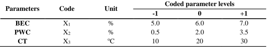
ranges and the levels of all the parameters investigated are given in Table 1.

Table 1: Independent parameters and their coded levels for CCD.

Parameters Code Unit Coded parameter levels

-1 0 +1

BEC X1 % 5.0 6.0 7.0

PWC X2 % 0.5 2.0 3.5

CT X3 oC 10 20 30

(-1) refers low level; (0) refers to mean level; (+1) refers to high level

7

(ITS) were performed in order to evaluate the mechanical properties. Air voids and dry density were measured to assess the volumetric properties, calculated according to Asphalt Institute [5] recommendations.

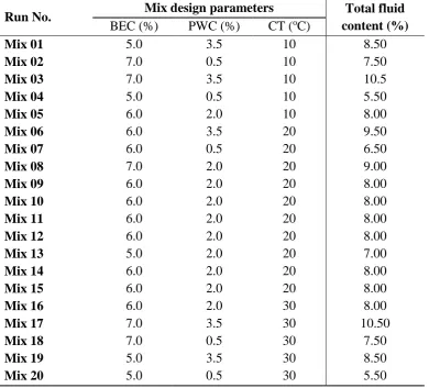
The total number of experiments carried out was 20 (= 2k +2k +6), where k is the number of parameters (k= 3). Fourteen different combinations were supplemented with six replicates of the mean case. The set of 14 mixes considered three levels of each studied parameter; all factors were varied in this way. The set of six replicates mixes considered the mid-level of each studied parameter; this point is often replicated in order to improve the precision of the experiment and minimize any possible sources of bias. The CCD matrix employed is presented in Table 2.

Table 2: Matrix of experimental design by CCD.

Run No. Mix design parameters Total fluid

content (%)

BEC (%) PWC (%) CT (oC)

Mix 01 5.0 3.5 10 8.50

Mix 02 7.0 0.5 10 7.50

Mix 03 7.0 3.5 10 10.5

Mix 04 5.0 0.5 10 5.50

Mix 05 6.0 2.0 10 8.00

Mix 06 6.0 3.5 20 9.50

Mix 07 6.0 0.5 20 6.50

Mix 08 7.0 2.0 20 9.00

Mix 09 6.0 2.0 20 8.00

Mix 10 6.0 2.0 20 8.00

Mix 11 6.0 2.0 20 8.00

Mix 12 6.0 2.0 20 8.00

Mix 13 5.0 2.0 20 7.00

Mix 14 6.0 2.0 20 8.00

Mix 15 6.0 2.0 20 8.00

Mix 16 6.0 2.0 30 8.00

Mix 17 7.0 3.5 30 10.50

Mix 18 7.0 0.5 30 7.50

Mix 19 5.0 3.5 30 8.50

8

3. Material and experimental procedures

3.1. Aggregate

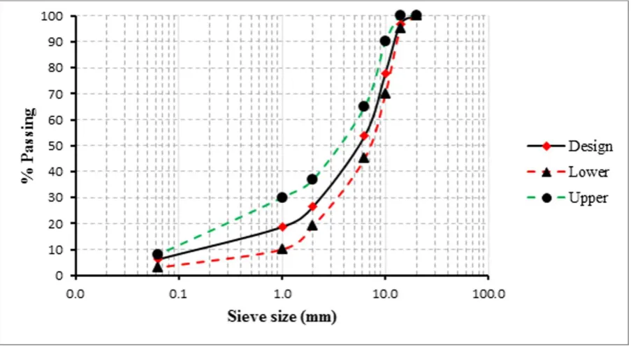
The aggregate used in this study was crushed limestone. The aggregate gradation used is shown in Fig. 1. In order to ensure appropriate interlocking of the dense graded surface course mix, a gradation was selected according to BS 4987-1 [32].

Fig. 1. Limestone aggregate gradation.

The physical properties of the limestone aggregate are shown in Table 3.

Table 3: Physical characteristics of limestone aggregate.

Properties Value

Density- Oven Dried 2.68 Mg/m3

Density- Saturated Surface Dried 2.69 Mg/m3

Density- Apparent 2.70 Mg/m3

Water Absorption 0.4 %

Aggregate Abrasion Value (AAV) 11.0

Polished Stone Value (PSV) 31

9

3.2. Bitumen Emulsion

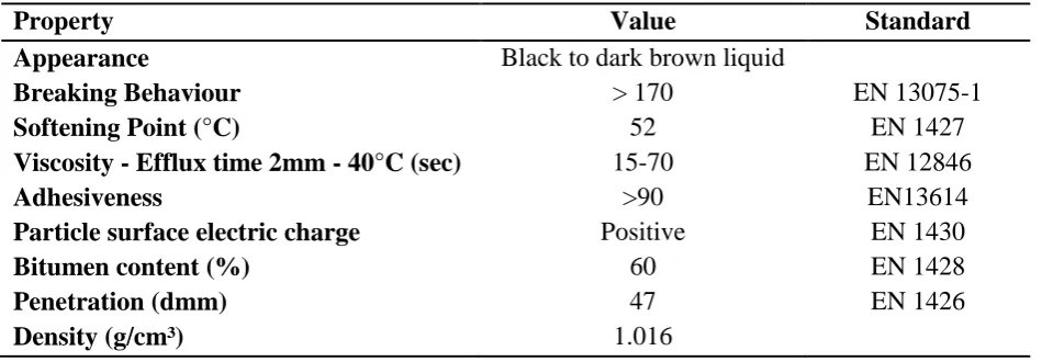
The binder used was cationic slow setting bituminous emulsion (C60B5) to ensure high adhesion between aggregate particles [1]. The relevant properties of the selected bituminous emulsion are shown in Table 4.

Table 4: Bitumen emulsion properties.

Property Value Standard

Appearance Black to dark brown liquid

Breaking Behaviour > 170 EN 13075-1

Softening Point (°C) 52 EN 1427

Viscosity - Efflux time 2mm - 40°C (sec) 15-70 EN 12846

Adhesiveness >90 EN13614

Particle surface electric charge Positive EN 1430

Bitumen content (%) 60 EN 1428

Penetration (dmm) 47 EN 1426

10

3.3. Sample manufacturing

The mix proportions presented in Table 2 were used to prepare Marshall specimens.

The procedure followed for preparing the specimens was such that the PWC was first added to the dry batched mixture and mixed using a Sun and Planet mixer for 60s. This was followed by mixing using a spatula for 30s ensuring that the aggregate materials were thoroughly blended and wetted ready for the addition of the bitumen emulsion. The required emulsion was subsequently added and the mixture mixed for another 60s. To ensure homogeneity and consistency in the mix, the materials were then mixed by hand using a spatula for 30s. These timings were found suitable for such mixes by [31, 33]. Impact compaction (Marshall Hammer) was utilized to compact the specimens; 75 blows applied to each face. The selection of 75 blows was made based on a pilot study performed to investigate the effective compaction effort for CBEMs. After compaction, the curing protocol followed was such that the specimens were left in the moulds for 24hrs (in a sealed condition) at the same ambient temperature before they were carefully extruded. After that, specimens were conditioned for 28 days in a thermostatically controlled air chamber at temperatures of 10oC, 20oC, and 30oC as stated in Table 2.

3.4. Laboratory testing program

11

3.4.1. Mechanical responses

The mechanical responses were evaluated by using ITSM and ITS tests.

Indirect tensile stiffness modulus

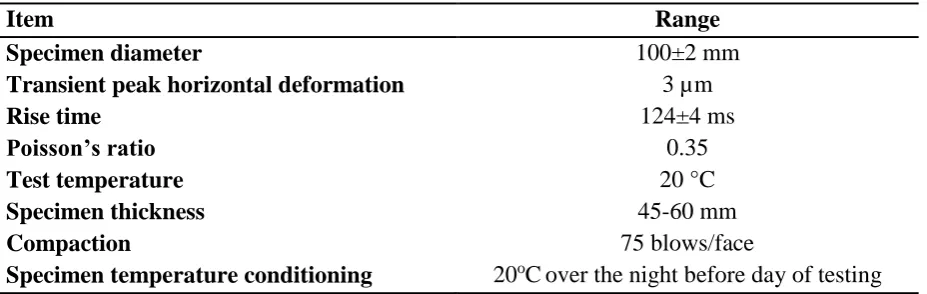
The ITSM is a non-destructive test used mainly to evaluate the stiffness modulus of bituminous mixes. Stiffness modulus is considered as an indicator of the structural behaviour of mixtures because it is related to the capacity of the material to distribute traffic loads. The test was carried out according to BS EN 12697-26 [34] and was performed under the conditions presented in Table 5. Four specimens per mix were tested under the same conditions.

Table 5: ITSM test conditions.

Item Range

Specimen diameter 100±2 mm

Transient peak horizontal deformation 3 µm

Rise time 124±4 ms

Poisson’s ratio 0.35

Test temperature 20 °C

Specimen thickness 45-60 mm

Compaction 75 blows/face

Specimen temperature conditioning 20oCover the night before day of testing

Indirect tensile strength

12

3.5. Volumetric responses

It was demonstrated by Thanaya [1] that satisfactory volumetric properties are essential to the design of CBEMs. The volumetric properties of mixes were evaluated using the methodology proposed by the Asphalt Institute [5].

4. Results and discussion

13

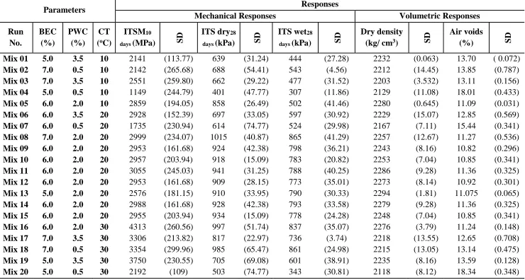
Table 6: Experimental factors and experimental responses

Parameters Responses

Mechanical Responses Volumetric Responses

Run No. BEC (%) PWC (%) CT (o_C)

ITSM10

days (MPa) SD

ITS dry28

days (kPa) SD

ITS wet28

days (kPa) SD

Dry density

(kg/ cm3₎ SD

Air voids

(%) SD

Mix 01 5.0 3.5 10 2141 (113.77) 639 (31.24) 444 (27.28) 2232 (0.063) 13.70 ( 0.072)

Mix 02 7.0 0.5 10 2142 (265.68) 688 (54.41) 543 (4.56) 2212 (14.45) 13.85 (0.787)

Mix 03 7.0 3.5 10 2551 (259.80) 662 (29.22) 477 (31.52) 2203 (3.532) 13.11 (0.156)

Mix 04 5.0 0.5 10 1149 (244.79) 401 (47.77) 307 (11.86) 2129 (11.08) 18.01 (0.433)

Mix 05 6.0 2.0 10 2859 (194.05) 858 (26.49) 502 (41.46) 2280 (0.645) 11.09 (0.031)

Mix 06 6.0 3.5 20 2928 (152.39) 697 (33.05) 597 (30.92) 2229 (15.07) 12.85 (0.569)

Mix 07 6.0 0.5 20 1735 (230.94) 614 (74.77) 524 (29.98) 2167 (7.11) 15.44 (0.341)

Mix 08 7.0 2.0 20 2999 (234.07) 1015 (40.87) 865 (41.29) 2257 (12.67) 11.27 (0.536)

Mix 09 6.0 2.0 20 2953 (161.68) 924 (42.38) 798 (36.21) 2243 (8.16) 10.82 (0.296)

Mix 10 6.0 2.0 20 2957 (203.94) 918 (15.09) 783 (20.82) 2253 (7.04) 10.85 (0.341)

Mix 11 6.0 2.0 20 3055 (245.03) 941 (31.25) 788 (40.25) 2286 (9.28) 11.36 (0.325)

Mix 12 6.0 2.0 20 2953 (161.68) 909 (28.15) 773 (35.01) 2273 (8.14) 10.92 (0.301)

Mix 13 5.0 2.0 20 2576 (181.15) 910 (33.95) 790 (30.33) 2294 (1.81) 11.075 (0.065)

Mix 14 6.0 2.0 20 2988 (161.68) 928 (42.38) 793 (33.58) 2279 (9.28) 11.36 (0.325)

Mix 15 6.0 2.0 20 2955 (203.94) 934 (15.09) 778 (24.28) 2248 (7.04) 10.85 (0.341)

Mix 16 6.0 2.0 30 4313 (260.56) 997 (51.74) 837 (35.07) 2276 (3.79) 11.24 (0.148)

Mix 17 7.0 3.5 30 3306 (213.82) 817 (22.97) 736 (3.74) 2218 (13.55) 12.65 (0.708)

Mix 18 7.0 0.5 30 3354 (299.96) 985 (65.47) 861 (24.98) 2215 (13.05) 13.14 (0.475)

Mix 19 5.0 3.5 30 3750 (230.55) 705 (69.08) 601 (38.91) 2235 (8.16) 13.59 (0.128)

Mix 20 5.0 0.5 30 2192 (109) 503 (74.77) 343 (30.81) 2118 (8.12) 18.34 (0.348)

14

4.1.Analysis of mechanical responses

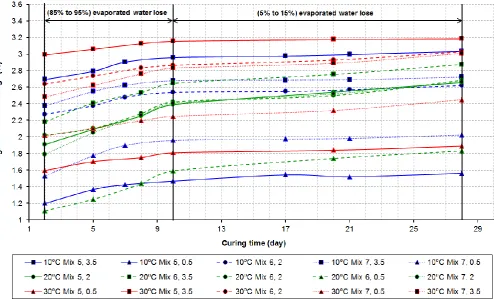
CMA performance is influenced by the time and temperature of the curing process [36-38].

Doyle et al. [36] found that it was necessary to vary both time and temperature of curing in order to represent the material achieved in the field. Logically, measurement of evaporated water will enable a better understanding of the performance of these mixtures. Therefore, periodically, specimen weights were recorded over 28 days. The results of average loss of water for all 15 individual mixes are shown in Fig. 2, in which for example (10o_{C Mix 5, 3.5)}

refers to curing at 10oC with 5% BEC and 3.5% PWC. The percentage of water loss was calculated based on the weight of specimens after demoulding directly. It can be observed that around 85% to 95% of the total evaporation occurs during the first 10 days and 5% to 15% through the remainder of the period.

15

The evaluation of stiffness was performed at 10 days and 28 days. This is broadly consistent with South African Bitumen Association [39] recommendation to evaluate CBEMs at room temperature at 7 days and 28 days.

4.1.1. Indirect tensile stiffness modulus

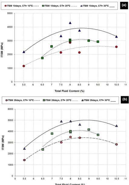
This test has often been used as an indicative test for ranking CBEMs during mix design [1, 31]. Following a conventional mix design method [5], the performance of CBEM was initially evaluated based on the relationship between total fluid content, which is the sum of BEC and PWC, and mechanical properties. The ITSM10 days and ITSM28 days are plotted

16

Fig. 3. The relation between ITSM and total fluid content of CBEMs under different CT

17

18

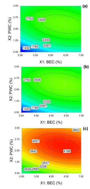
Fig. 4. Contour plots of ITSM10 days versus BEC and PWC; (a) CT =10oC, (b) CT =20oC

19

The results in Fig. 4 show the effect of BEC and PWC versus ITSM10 days at different CT.

From these contour plots ITSM10 days values tend to increase markedly with increasing PWC

from 0.50% to 2.75% and with increasing BEC from 5.0% to 6.5%. However, ITSM10 days

markedly decreases when increasing PWC from 2.75% to 3.5% and increases slightly when increasing BEC from 6.5% to 7.0%. Moreover, the results in Fig. 4 show that in reality the individual effects of BEC and PWC are important, rather than simply total fluid content. The response surface presented in Fig. 4 shows elliptical contours which is the pattern obtained when there are perfect interactions between independent variables [41, 42]. Accordingly, there is a region of optimum performance at around 6.0- 6.5% BEC and 2.0- 2.5% PWC, whereas ITSM is lower with different BEC/ PWC proportions, even at the same total fluid content. The effect of increasing CT is to increase ITSM(by approximately 1.25-1.60 times as the CT increases from 10o_{C to 30}o_{C) but optimum BEC and PWC are not significantly}

affected.

4.1.2. Indirect tensile strength

20

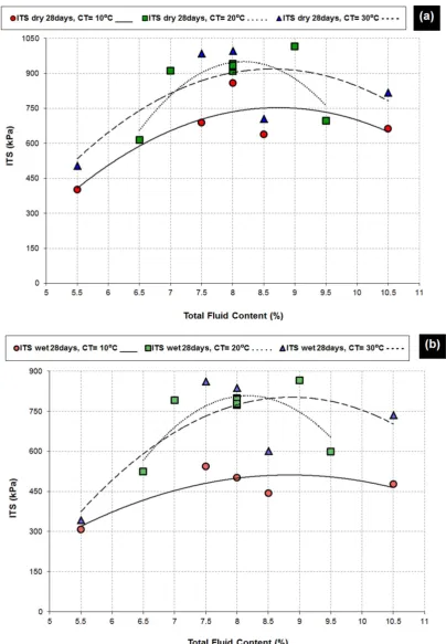
Fig. 5. The relation between ITS and total fluid content of CBEMs under different CT

(a) dry condition and (b) wet condition.

21

Fig. 6. Contour plots of ITS dry28 days versus BEC and PWC; (a) CT =10oC, (b) CT

22

Fig. 7. Contour plots of ITS wet28 days versus BEC and PWC; (a) CT =10oC, (b) CT

23

From Fig. 6 and 7, at a given CT, the results again indicate that ITS values significantly increase by increasing PWC from 0.50% to 2.375% and always increase with BEC while they markedly decrease by increasing the PWC from 2.375% to 3.5%. Over all, increasing ITS was observed by increasing BEC and CT. The response surface presented in Fig. 6 and 7 shows distorted parabolic contours which are obtained in cases with fewer interactions between independent variables [41, 42]. This means that the optimum region is less clear than was the case of ITSM. Optimum PWC is between 1.5- 2.5%, but optimum BEC may be around 6.5- 7.0% or higher. The effect of CT on these optimum is again slight and both dry and wet data sets present a similar picture. A more general conclusion from both ITSM and ITS, is that the interaction of BEC and PWC (and to a lesser extent CT) is complex and that CBEMs must be carefully and accurately designed. This conclusion is consistent with the findings of Gómez-Meijide and Pérez [2].

4.2. Analysis of volumetric responses

A volumetric analysis was carried out to determine the void content and dry density present in each mix.

4.2.1. Air voids:

24

Fig. 8. The relation between air voids and total fluid content of CBEMs.

The highest values of air voids were observed at the lowest total fluid content, whereas the lowest air voids values were found at 8% to 9% total fluid content. The results imply the role of fluid inside the CBEM to determine the degree of compatibility of mixes.

25

Based on RSM modelling, Fig. 9 presents a contour plot for the air voids measurement in which it is clear that the individual effects of BEC and PWC are both important. Air voids values decreased when increasing the BEC from 5.0% to 7.0% and markedly decreased when increasing the PWC from 0.50% to 2.0% then significantly increased when increasing PWC from 2.0% to 3.5%. As for ITS there is a clear optimum region for PWC, about 1.5- 2.5%, but optimum BEC would appear to be at 7% or more and is therefore less clear on the plot. It is evident that PWC plays a key role in determining air voids in CBEM.

4.2.2. Dry density:

The dry density results are shown in Table 6. Fig. 10 presents the relation between dry density and total fluid content. Dry density values peak at around 8 to 9% total fluid content.

Fig. 10. The relation between dry density and total fluid content of CBEMs.

26

Fig. 11. Contour plot of dry density versus BEC and PWC.

Fig. 11 indicates that the dry density of CBEMs increased dramatically with an increase of PWC from 0.50% to 2.375% then decreased with an increase of PWC from 2.375% to 3.5%. The dry density slightly increased when BEC increased from 5.0% to 7.0%. The optimum PWC is in a narrow band either side of 2%, while optimum BEC is less definite but appears to be close to 7%. Low dry density corresponds to high air voids and poor mechanical performance, while the optimum for each measure approximately coincides.

4.3. Statistical analysis of responses

A statistical analysis was conducted to evaluate mix performance in terms of the above-mentioned tests. A quadratic model was developed for prediction purposes. The quality of the developed model was evaluated based on the coefficient of determination, R2 _{and also the}

27

For a good model fit, the coefficient of determination should be a minimum of 0.80. A high R2 _{value close to 1.00 demonstrates a desirable and reasonable agreement between the}

calculated and observed results [43].

An additional tool used to evaluate the developed model was ‘‘adequate precision’’ (AP). AP

compares the range of the predicted values at the design points to the average prediction error. In this particular case, the AP values of the models were 29.3, 35.3, 21.1, 28.5 and 17.6 for, respectively. They are greater than 4 and therefore confirm that the model can be used to navigate the space defined by the CCD [12].

The results of ANOVA analysis presented in Table 7 show that the models’ F-values of 44.76, 94.77, 32.64, 77.77 and 36.82 and low P-values, which mean that the models are statistically significant for ITSM10 days, ITS dry28 days, ITS wet28 days, air voids and dry density,

respectively. Only a 0.01% chance exists that a model F-value of this magnitude can occur because of noise.

ANOVA results confirm that all the main parameters in the mix design of CBEMs (BEC (X1),

PWC (X2) and CT (X3)) have significant effects on mechanical response according to the

t-test at a 5% significance level (P < 0.05). Both BEC and PWC have a significant effect on

28

Table 7: ANOVA for analysis of variance and adequacy of the quadratic model for

responses.

Response SoD SoS DoF MS F-value P-value>F Comment

ITSM 10 days

Model 8.88E+06 7 1.27E+06 44.76 < 0.0001

SD= 168.34 Mean= 2792.8 R2 _{= 0.96}

Adj. R2 = 0.94 AP =29.2

X1 6.47E+05 1 6.47E+05 22.84 0.0004

X2 1.68E+06 1 1.68E+06 59.44 < 0.0001

X3 3.69E+06 1 3.69E+06 130.15 < 0.0001

X12 1.78E+05 1 1.78E+05 6.27 0.0277

X22 1.39E+06 1 1.39E+06 48.94 < 0.0001

X32 8.15E+05 1 8.15E+05 28.76 0.0002

X1 X2 5.99E+05 1 5.99E+05 21.14 0.0006

Residual 3.40E+05 12 28338.13

Lack of Fit 3.318 E+05 7 47402.40 28.76 0.0010

Pure Error 8240.83 5 1648.17

ITS dry28 days

Model 5.81E+05 8 72628.92 94.77 < 0.0001

SD= 27.68 Mean= 802.25 R2 _{= 0.98}

Adj. R2 = 0.97 AP =35.3

X1 1.02E+05 1 1.02E+05 132.84 < 0.0001

X2 10824.1 1 10824.1 14.12 0.0032

X3 57608.1 1 57608.1 75.17 < 0.0001

X12 2497.61 1 2497.61 3.26 0.0985

X22 2.49E+05 1 2.49E+05 325.16 < 0.0001

X1 X2 50244.5 1 50244.5 65.56 < 0.0001

X1 X3 10082 1 10082 13.16 0.004

X2 X3 3960.5 1 3960.5 5.17 0.0441

Residual 8430.39 11 766.4

Lack of Fit _7781.05 6 1296.84 9.99 0.0116

Pure Error 649.33 5 129.87

ITS wet28 days

Model 5.767E+005 8 72081.68 32.64 < 0.0001 SD= 46.99 Mean= 656.95 R2 = 0.95

X1 99496.64 1 99496.64 45.06 < 0.0001

29

X3 1.223E+005 1 1.223E+005 55.38 < 0.0001 Adj. R2 = 0.93

AP =21.1

X12 10170.78 1 10170.78 4.61 0.0550

X22 1.163E+005 1 1.163E+005 52.66 < 0.0001

X32 25776.15 1 25776.15 11.67 0.0058

X1 X2 43087.27 1 43087.27 19.51 0.0010

X1 X3 18294.98 1 18294.98 8.29 0.0150

Residual 24289.82 11 2208.17

Lack of Fit 23837.05 6 3972.84 43.87 0.0004

Pure Error 452.77 5 90.55

Air voids

Model 92.97 4 23.24 77.77 < 0.0001

SD= 0.55 Mean= 12.78 R2 = 0.95 Adj. R2 = 0.94 AP = 28.5

X1 11.44 1 11.44 38.28 < 0.0001

X2 16.59 1 16.59 55.51 < 0.0001

X22 57.27 1 57.27 191.66 < 0.0001

X1 X2 7.66 1 7.66 25.65 < 0.0001

Residual 4.48 15 0.30

Lack of Fit 4.14 10 0.41 6.12 0.0295

Pure Error 0.31 5 0.062

Dry Density

Model 41661.05 4 10415.26 36.82 < 0.0001

SD= 16.82 Mean= 2232.35 R2 = 0.90 Adj. R2 _{= 0.88}

AP = 17.6

X1 940.90 1 940.90 3.33 0.0882

X2 7617.60 1 7617.60 26.93 0.0001

X22 26718.05 1 26718.05 94.44 < 0.0001

X1 X2 6384.50 1 6384.50 22.57 0.0003

Residual 4243.50 15 282.90

Lack of Fit 2636.17 10 263.62 0.82 0.6321

Pure Error 1607.33 5 321.47

SoD: source of data; SoS: sum of squares; DoF: degree of freedom; MS: mean square.

X1 = BEC, X2 = PWC and X3 =CT

30

responses including ITSM10 days, ITS dry28 days, ITS wet28 days and air voids were significant. It

is worth noting that while LOF values were significant, reasonable agreement between the predicted and adjusted R2 were found for all responses such that it can be concluded that the suggested models for all responses can be used to navigate satisfactorily into design space to find optimum mix design parameters. Similar observations were reported by [23, 24, 44].

The final regression models, in terms of the significant influencing factors, are expressed by the following second-order polynomial equations:

𝐼𝑇𝑆𝑀_{10 𝑑𝑎𝑦𝑠} = −10708.36 + 3668.86𝑋₁+ 2630.56𝑋₂− 157.01𝑋₃− 254.13𝑋₁2

− 315.61𝑋₂2 _{+ 5.44𝑋}

32− 182.41𝑋1𝑋2 (2)

𝐼𝑇𝑆 𝑑𝑟𝑦28 𝑑𝑎𝑦 = 369.05 − 199.68𝑋1+ 864.71𝑋2− 10.74𝑋3+ 27.93𝑋12− 124.02𝑋22

− 52.83𝑋₁𝑋₂+ 3.55𝑋₁𝑋₃− 1.48𝑋₂𝑋₃ (3)

𝐼𝑇𝑆 𝑤𝑒𝑡_{28 𝑑𝑎𝑦}= 1344.55 − 627.82𝑋₁+ 677.51𝑋₂+ 21.09𝑋₃+ 60.81𝑋₁2_{+ 60.81𝑋} 22

− 0.96𝑋₃2_{− 48.92𝑋}

1𝑋2+ 4.78𝑋1𝑋3 (4)

𝐴𝑖𝑟 𝑣𝑜𝑖𝑑𝑠 = 33.06 − 2.37𝑋1− 10.79𝑋2+ 1.50𝑋22+ 0.65𝑋1𝑋2 (5)

𝐷𝑟𝑦 𝐷𝑒𝑛𝑠𝑖𝑡𝑦 = 2268.90 + 9.70𝑋₁+ 27.60 𝑋₂− 73.10𝑋₂2_{− 28.25𝑋}

1𝑋2 (6)

31

affects the mechanical and volumetric responses. As clear in Table 7, where the interactive term is not statistically significant, their surface plots were not represented in Fig. 12.

The curvature of the surface plot in Fig. 12 (a) indicates that both BEC and PWC have interaction effect on ITSM10 days. Also, Fig. 12 (b-f) depicts the effects of mix design

32

Fig. 12. 3D-surface plots of ITSM10 days, ITS dry28 days, ITS wet28 days, air voids and dry

density. (a) ITSM10 days versus BEC and PWC. (b) ITS dry28 days versus BEC and PWC. (c)

ITS dry28 days versus BEC and CT. (d) ITS dry28 days versus PWC and CT. (e) ITS wet28 days

versus BEC and PWC. (f) ITS wet28 days versus BEC and CT. (g) Air voids versus BEC and

33

4.4. Optimization the mix design components

An optimization process was carried out to determine the optimum value of BEC, and PWC under different CTs, using the Design Expert 9.0.6.2 software (Stat-Ease Inc., Minneapolis, USA). According to the software optimization step, the desired goal for each mix design parameter (BEC and PWC) was chosen within the range shown in Table 1. The desirable mechanical responses (ITSM10 days, ITS dry28 days and ITS wet28 days) were defined as being a

maximum to achieve the highest performance, the desirable air voids was defined as a minimum and desirable dry density was defined as a maximum in order to achieve a dense mixture with the lowest value of air voids. The derived second order polynomial models were used to interpolate the mix design parameters within the range and based on the desired responses. The results are presented in Table 8.

Table 8: The optimum BEC and PWC at different CT with their responses.

Items Model prediction Laboratory experiment

CT (o_{C) T= 10} o_{C T= 20} o_{C T= 30} o_{C T= 20} o_C

BEC (%) 7.00 6.75 6.58 6.75

PWC (%) 1.96 2.12 2.16 2.12

ITSM10 days (MPa) 2936 3063 4235 3049

ITS dry 28 days (kPa) 946 1015 1086 1000

ITS wet 28 days (kPa) 684 883 894 889

Air voids (%) 10.02 10.26 10.42 10.34

Dry density (kg/cm3_{) 2279 2276 2275 2278}

34

The results in Table 8 show a limited variation of optimum mix design proportions (BEC and PWC) over the range of CT from 10o_{C to 30}o_{C. The maximum variation of BEC is 0.42%}

and 0.20% for PWC. The total fluid content (BEC + PWC) for the optimized mixes lies within the range from 8.74% to 8.96%. Therefore, it can be concluded that the optimum proportions (BEC and PWC) tend to be only slightly influenced by CT. Overall, the results are comparable with those published by other authors about the mix design of CBEM [1, 26, 31].

5. Conclusions

The current research introduces a novel performance based mix design approach for CBEM involving mechanical and volumetric properties. A statistical approach was adopted in order to optimize the mix design parameters using RSM. Based on the laboratory experiments and analyses, the following conclusions can be drawn:

1. An alternative mix design approach for CBEMs was investigated using RSM. This approach involves the mechanical and volumetric properties. It was statistically demonstrated that the alternative approach output results were consistent with the laboratory tests.

2. The RSM approach offers a more comprehensive view of the effect of the variation of each mix design parameter on the mechanical and volumetric responses of CBEMs than would otherwise be the case. It has the advantage that all parameters are investigated at one time.

35

strength/ stiffness of CBEM at the same total fluid content and with different BEC/ PWC proportions.

4. The evaluation of stiffness modulus of CBEMs after 10 days is likely to give the designer appropriate information to optimize the mix design of CBEMs in a relatively short time. 5. Based on the optimization by RSM, it can be concluded that the optimum mix design

proportions (BEC and PWC) tend to be only slightly influenced by CT.

6. Acknowledgments

36

7. References

[1] Thanaya I. Improving the performance of cold bituminous emulsion mixtures (CBEMs): incorporating waste [PhD thesis]: University of Leeds, UK; 2003.

[2] Gómez-Meijide B, Pérez I. A proposed methodology for the global study of the mechanical properties of cold asphalt mixtures. Materials & Design. 2014;57(0):520-7. [3] Liebenberg J, Visser A. Towards a mechanistic structural design procedure for emulsion-treated base layers: technical paper. Journal of the South African Institution of Civil Engineering. 2004;46(3):p. 2-9.

[4] Brayton TE, Lee K, Gress D, Harrington J. Development of performance-based mix design for Cold in-Place Recycling of asphalt mixtures. 80th Annual Meeting of the Transportation Research Board. Washington, D.C.,USA 2000.

[5] Asphalt Institute. Asphalt Cold Mix Manual. Series No 14. Maryland, USA1989.

[6] Sebaaly PE, Bazi G, Hitti E, Weitzel D, Bemanian S. Performance of cold in-place recycling in Nevada. 83th Annual Meeting of the Transportation Research Board. Washington DC, USA 2004. p. 162-9.

[7] Kim Y, Lee HD, Heitzman M. Validation of new mix design procedure for cold in-place recycling with foamed asphalt. Journal of Materials in Civil Engineering. 2007;19(11):1000-10.

[8] Forth J, Zoorob S, Thanaya I. Development of bitumen-bound waste aggregate building blocks. Proceedings of the ICE-Construction Materials. London, UK 2006. p. 23-32.

[9] Montgomery DC. Design and analysis of experiments. 7 th ed. New York, USA: John Wiley & Sons, Inc; 2008.

[10] Khuri AI, Cornell JA. Response surfaces: designs and analyses. 2nd ed. New York, USA: Marcel Dekker, Inc; 1996.

[11] Bayramov F, Taşdemir C, Taşdemir MA. Optimisation of steel fibre reinforced concretes by means of statistical response surface method. Cement and Concrete Composites. 2004;26(6):665-75.

[12] Aldahdooh M, Muhamad Bunnori N, Megat Johari M. Evaluation of ultra-high-performance-fiber reinforced concrete binder content using the response surface method. Materials & Design. 2013;52:957-65.

[13] Bektas F, Bektas BA. Analyzing mix parameters in ASR concrete using response surface methodology. Construction and Building Materials. 2014;66:299-305.

[14] Faseeulla Khan MD, Dwivedi DK, Sharma S. Development of response surface model for tensile shear strength of weld-bonds of aluminium alloy 6061 T651. Materials & Design. 2012;34(0):673-8.

[15] Nekahi A, Dehghani K. Modeling the thermomechanical effects on baking behavior of low carbon steels using response surface methodology. Materials & Design. 2010;31(8):3845-51.

[16] Younesi M, Bahrololoom ME. Formulating the effects of applied temperature and pressure of hot pressing process on the mechanical properties of polypropylene– hydroxyapatite bio-composites by response surface methodology. Materials & Design. 2010;31(10):4621-30.

[17] Chávez-Valencia L, Manzano-Ramírez A, Luna-Barcenas G, Alonso-Guzmán E. Modelling of the performance of asphalt pavement using response surface methodology. Building and environment. 2005;40(8):1140-9.

37

[19] Hamzah MO, Golchin B, Tye CT. Determination of the optimum binder content of warm mix asphalt incorporating Rediset using response surface method. Construction and Building Materials. 2013;47:1328-36.

[20] Kavussi A, Qorbani M, Khodaii A, Haghshenas H. Moisture susceptibility of warm mix asphalt: A statistical analysis of the laboratory testing results. Construction and Building Materials. 2014;52:511-7.

[21] Khodaii A, Haghshenas H, Kazemi Tehrani H. Effect of grading and lime content on HMA stripping using statistical methodology. Construction and Building Materials. 2012;34:131-5.

[22] Khodaii A, Mousavi E, Khedmati M, Iranitalab A. Identification of dominant parameters for stripping potential in warm mix asphalt using response surface methodology. Materials and Structures. 2015:1-13.

[23] Hamzah MO, Omranian SR, Golchin B, Hainin MRH. Evaluation of Effects of Extended Short-Term Aging on the Rheological Properties of Asphalt Binders at Intermediate Temperatures Using Respond Surface Method. Jurnal Teknologi. 2015;73(4).

[24] Moghaddam TB, Soltani M, Karim MR, Baaj H. Optimization of asphalt and modifier contents for polyethylene terephthalate modified asphalt mixtures using response surface methodology. Measurement. 2015;74:159-69.

[25] Ameri M, Sanij HK, Toolabi S, Hosseini SH. Optimization of The Cold In-Place Recycling Mix Design by Nonlinear Simplex Method. Transportation Research. 2012;2(1):1. [26] Gómez-Meijide B, Pérez I. Effects of the use of construction and demolition waste aggregates in cold asphalt mixtures. Construction and Building Materials. 2014;51(0):267-77. [27] Jenkins K, Moloto P. Updating bituminous stabilized materials guidelines: mix design report. Phase II–Curing protocol: improvement. Technical memorandum task 7; 2008.

[28] Loizos A. In-situ characterization of foamed bitumen treated layer mixes for heavy-duty pavements. International Journal of Pavement Engineering. 2007;8(2):123-35.

[29] Konrad J-M, Walter J. Influence of curing on the mechanical properties of a dense graded emulsion mix. Road Materials and Pavement Design. 2001;2(2):181-94.

[30] Ojum C, Kuna K, Thom NH, Airey G. An investigation into the effects of accelerated curing on Cold Recycled Bituminous Mixes. International Conference on Asphalt Pavements, ISAP. North Carolina, USA 2014. p. 1177-88.

[31] Oke OL. A study on the development of guidelines for the production of bitumen emulsion stabilised RAPs for roads in the tropics [PhD thesis]: University of Nottingham, UK; 2011.

[32] European Committee for Standarization. BS 4987-1: Coated macadam (asphalt concrete) for roads and other paved areas. Part 1: Specification for constituent materials and for mixtures. London, UK British Standards Institution; 2005.

[33] Sunarjono S. The influence of foamed bitumen characteristics on cold-mix asphalt properties [PhD Thesis]: University of Nottingham, UK; 2008.

[34] European Committee for Standarization. BS EN 12697-26: Bituminous mixtures: Test methods for hot mix asphalt. Part 26: Stiffness. London, UK British Standards Institution; 2012.

[35] European Committee for Standarization. BS EN 12697-23:Test methods for hot mix asphalt. . Part 23: Determination of the indirect tensile strength of bituminous specimens. London, UK British Standards Institution; 2003.

[36] Doyle T, Gibney A, Mcnally C, Tabakovic A. Developing maturity methods for the assessment of cold-mix bituminous materials. Construction and Building Materials. 2013;38:524-9.

38

[38] García A, Lura P, Partl MN, Jerjen I. Influence of cement content and environmental humidity on asphalt emulsion and cement composites performance. Materials and structures. 2013;46(8):1275-89.

[39] South African Bitumen Association. ETB–The design and use of emulsion-treated bases. SABITA Manual 21. Cape Town, South Africa 1999.

[40] Al-Busaltan S, Al Nageim H, Atherton W, Sharples G. Mechanical Properties of an Upgrading Cold-Mix Asphalt Using Waste Materials. Journal of Materials in Civil Engineering. 2012;24(12):1484-91.

[41] Wang J-P, Chen Y-Z, Wang Y, Yuan S-J, Yu H-Q. Optimization of the coagulation-flocculation process for pulp mill wastewater treatment using a combination of uniform design and response surface methodology. Water Research. 2011;45(17):5633-40.

[42] Muralidhar R, Chirumamila R, Marchant R, Nigam P. A response surface approach for the comparison of lipase production by Candida cylindracea using two different carbon sources. Biochemical Engineering Journal. 2001;9(1):17-23.

[43] Noordin MY, Venkatesh VC, Sharif S, Elting S, Abdullah A. Application of response surface methodology in describing the performance of coated carbide tools when turning AISI 1045 steel. Journal of Materials Processing Technology. 2004;145(1):46-58.