Practical quantum metrology in noisy environments
Rosanna Nichols, Thomas R. Bromley, Luis A. Correa, and Gerardo Adesso*
School of Mathematical Sciences, The University of Nottingham, University Park, Nottingham NG7 2RD, United Kingdom (Received 8 April 2016; published 3 October 2016)
The problem of estimating an unknown phaseϕusing two-level probes in the presence of unital phase-covariant noise and using finite resources is investigated. We introduce a simple model in which the phase-imprinting operation on the probes is realized by a unitary transformation with a randomly sampled generator. We determine the optimal phase sensitivity in a sequential estimation protocol and derive a general (tight-fitting) lower bound. The sensitivity grows quadratically with the number of applicationsNof the phase-imprinting operation, then attains a maximum at someNopt, and eventually decays to zero. We provide an estimate ofNopt in terms of
accessible geometric properties of the noise and illustrate its usefulness as a guideline for optimizing the estimation protocol. The use of passive ancillas and of entangled probes in parallel to improve the phase sensitivity is also considered. We find that multiprobe entanglement may offer no practical advantage over single-probe coherence if the interrogation at the output is restricted to measuring local observables.
DOI:10.1103/PhysRevA.94.042101
I. INTRODUCTION
Advances in metrology are pivotal to improve measurement standards, to develop ultrasensitive technologies for defense and health care, and to push the boundaries of science, as demonstrated by the detection of gravitational waves [1]. In a typical metrological setting, an unknown parameter ϕ is dynamically imprinted on a suitably prepared probe. We can think, e.g., of a two-level spin undergoing a unitary phase shift, ˆU =exp{−iH ϕˆ }. By subsequently interrogating the probe, one builds an estimate ϕest for the parameter [2–4]. The corresponding mean-square errorδ2ϕ ≡ (ϕest−ϕ)2can be reduced, for instance, by using N uncorrelated identical probes. In that case,δ2ϕscales asymptotically as 1/N, which is referred to as the standard quantum limit [2]. However, if thoseN probes were prepared in an entangled state, the resulting uncertainty could be further reduced by an additional factor ofN, leading toδ2ϕ∼1/N2. This ultimate quantum enhancement in resolution is termed Heisenberg limit and is highly sought after in quantum metrology [3].
In practice, the unitary dynamics of the probe will be distorted by noise, due to unavoidable interactions with its surroundings. Unfortunately, the metrological advantage of entangled probes over separable ones vanishes for most types of uncorrelated noise, such as spontaneous emission, depolarizing noise [5], or phase damping [6,7]. Entanglement may remain advantageous though, provided one gains precise control over the noise strength, and only for limited cases such as time-inhomogeneous phase-covariant noise [8–12], transversal noise [13,14], or when error-correction protocols may be used [15,16]. Creating entangled states with a large number of particles is nevertheless a costly process, limited by technological constraints [17]. Furthermore, to fully harness the metrological power of entanglement in the presence of noise, collective measurements on all N probes at the output would be generally required [18]. This contrasts with the noiseless scenario, in which separable measurements
(i.e., performed locally on each probe) suffice to attain the Heisenberg scaling [3].
One can try to circumvent these problems by devising an alternative sequentialor “multiround” strategy, in which the parameter-imprinting unitary acts N consecutive times on a single probe before performing the final measurement. In the absence of noise, this sequential setting is formally equivalent to the parallel one [19], the only difference being that quantumcoherence[20–23] takes over the instrumental role of entanglement. The sequential scheme seems more appealing from a practical viewpoint, as only a single probe needs to be addressed in both state preparation and final interrogation [24]. However, the Heisenberg scaling of the precision cannot be maintained asymptotically in the sequential scenario either, once again due to the detrimental effects of noise.
In Sec. IV we then illustrate our results by choosing a specific distribution for the stochastic generator. We compare the QFI in the sequential setting (with and without passive correlated ancillas) with the actual phase sensitivity of given feasible measurements. For completeness, we also compute the QFI analytically in a parallel-entangled setting starting from an N-qubit GHZ state. Although the QFI exhibits an asymptotic linear scaling in N in such setting, we find that entangled probes may provide no practical advantage when their interrogation is restricted to measurements of local observables on each individual qubit. In fact, in such case the sensitivity for the parallel-entangled strategy reduces to that of the sequential one, where the “number of probes” comes to play the role of the “number of rounds.” Our analysis, summarized in Sec.V, reveals feasible solutions for quantum metrology based on the little-studied sequential paradigm (possibly supplemented by a passive ancilla), robust even under sizable levels of noise.
II. THE NOISE MODEL A. Uncertain phase generator
Let us start by introducing our model for ease of illustration. In the sequential scenario, a two-level probe undergoes a sequence ofN phase shifts, ˆUn=exp{−iϕHˆn}, before being
interrogated. The generator can be written as ˆHn=n·σ,
where the axisn=(sinθcosφ,sinθsinφ,cosθ) is sampled from some normalized probability distribution p(θ,φ) and σ is the vector of the three Pauli matrices. Thus the phase-imprinting operationϕ, which transforms the probe state at each step, is
ˆ
N =ϕNˆ −1≡
π
0 dθ
2π
0
dφUˆnNˆ −1Uˆn†p(θ,φ) sinθ.
(1)
The resulting qubit channel is completely positive, trace preserving,unital(i.e.,ϕ1=1), and contractive [26], i.e., any state will be asymptotically mapped to ˆ∞→ 121; note also that Eq. (1) is akin to the classical simulation method of Ref. [5]. Without loss of generality, we may take the average rotation axis n =dθdφnp(θ,φ) sinθ proportional to (0,0,1), hence restricting to probability distributions p(θ) with axial symmetry on the Bloch sphere, so that our
qubit channel ϕ is phase covariant, as it commutes with ˆ
Hn[11].
Physically, we may think, for instance, of the free evolution of a nuclear spin with gyromagnetic ratio γ in an external magnetic field B pointing along z. In that case, ˆH = γ2σzˆ , so thatϕ =γ2Bt, wheret k
BT is some coarse-grained
time resolution, of the same order as the thermal fluctuations of the environment. The interactions with the surrounding nuclei at large temperatures result in random changes of the net direction of the magnetic field on our spin. This gives rise to a relaxation process towards the thermal equilibrium state ˆτT 121. If the direction ofB were kept fixed and the environmental effects were accounted for by a fluctuating mag-netic field intensityB, the model would realize pure dephasing instead [27], which is often dominant at short-time scales.
B. General unital phase-covariant qubit channels While the model in Eq. (1) can be conveniently adopted as a physical example to focus our analysis, the results derived in this paper will hold for a more general class of channels, namely all the unital phase-covariant qubit channels, whose description is recalled here.
Given a single-qubit state ˆ= 12(1+r·σ), any single-qubit channel maps the Bloch vectorrintor =R r+t, where Ris a 3×3 real distortion matrix andtis a displacement vec-tor. For the most general unital phase-covariant channel [28], t=0and
R(ϕ)=
⎛
⎝λλ⊥⊥((ϕϕ) cos) singg((ϕϕ)) −λλ⊥⊥(ϕ(ϕ) cos) singg((ϕϕ)) 00
0 0 λ(ϕ)
⎞ ⎠. (2)
These channels encode information aboutϕ not only in the rotation of the Bloch ball by a function g(ϕ), but also in its deformation, through the singular values ofR(ϕ), namely λ(ϕ) and the doubly degenerate λ⊥(ϕ), which must satisfy λ1 and 2λ⊥ 1+λ(implyingλ⊥1) for the map to be completely positive [29]. Equation (2) thus generalizes the canonical phase-covariant channels such as phase damping, for which g(ϕ)=ϕ [11]. In what follows, we shall work with the 4×4 Liouville representation K(ϕ), which acts on vectorizations|ˆ ≡(0|ˆ|0,0|ˆ|1,1|ˆ|0,1|ˆ|1) of any density matrix ˆ in the computational basis as |ˆ →
K(ϕ)|ˆ, whereK(ϕ) is written as
K(ϕ)=1 2
⎛ ⎜ ⎜ ⎝
1+λ(ϕ) 0 0 1−λ(ϕ)
0 2λ⊥(ϕ)e−ig(ϕ) 0 0 0 0 2λ⊥(ϕ)eig(ϕ) 0
1−λ(ϕ) 0 0 1+λ(ϕ)
⎞ ⎟ ⎟
⎠. (3)
III. PHASE SENSITIVITY A. Quantum Fisher information
We will now analyze the sensitivity for estimating a phase imprinted by any unital phase-covariant qubit channel, starting with the sequential estimation setting. Recall that the estimate ϕestis built by measuring some observable ˆOon the final state of the probe ˆNafterNsuccessive applications of the channel.
We can then gauge the phase sensitivity of ˆOas
FOˆ ≡ ∂ϕOˆ 2
2Oˆ , (4)
observable ˆO(assumed nondegenerate) [30]. In particular, one can verify that equality holds for all the explicit examples presented later in the paper, and henceforth we shall simply refer toFOˆ as the phase sensitivity associated to the (generally suboptimal) observable ˆO.
The QFI F, which captures geometrically the rate of change of the evolved probe state ˆN under an infinitesimal variation of the parameterϕ, corresponds to the classical Fisher information of an optimal observable (i.e., F =supOˆ I
ˆ O) and is thus a meaningful benchmark for the best estimation protocol. Such an optimal observable is diagonal in the eigenbasis of the symmetric logarithmic derivative (SLD) ˆL, defined implicitly by [31]
ˆ
LNˆ +Nˆ Lˆ ≡2∂ϕNˆ . (5)
Note that the prominent role of the QFI F in quantum estimation theory is well established in an asymptotic setting, by virtue of its appearance in the quantum Cram´er-Rao bound [25],δ2ϕ 1/(MF), which becomes tight in the limit of a large numberM1 of independent repetitions. However, the QFI also enters in both the van Trees inequality [32] and the Ziv-Zakai bound [33], which can provide tighter and more versatile bounds on the mean-square errorδ2ϕin the relevant case of finiteM(including Bayesian settings). Therefore, we shall adopt the QFI as our main figure of merit, in keeping with the quantum metrology bulk literature (see, e.g., [34] for a recent discussion) and in compliance with the spirit of this paper, which focuses on the use of finite resources to retain quantum enhancements in the estimation sensitivity. We will also assume maximization ofF over the initial state of the probe unless stated otherwise.
To calculate the QFIFN(ϕ), we make use of the formula
FN(ϕ)=4
i,j qi
(qi+qj)2|ψi|∂ϕˆN|ψj|
2, (6)
where |ψi and qi are, respectively, the eigenvectors and eigenvalues of ˆN [35,36] (excluding terms withqi+qj =0 from the sum), and we have made the dependence of the QFI on ϕ and N explicit. By preparing the probe in the optimal, maximally coherent state|+ =(|0 + |1)/√2 [19], we obtain exactly
FN(ϕ)=N2
λ2⊥N(∂ϕg)2+(∂ϕλ⊥) 2λ2N−2
⊥ 1−λ2N ⊥
. (7)
The QFI thus grows as∼N2for smallN, reaches a peak at some Nopt, and then decays asymptotically to zero. A similar qualitative behavior has been recently reported under other types of (nonunital) noise, such as erasure, spontaneous emission, and phase damping [37,38].
B. Optimal “sampling time”
In order to optimize our sequential protocol, we need a practical way to determine Nopt. To that end, we aim to bound the QFI from below. In general, one may use maxˆˆ|(∂ϕKN)†∂ϕKN|ˆFN(ϕ) [38,39], which is not necessarily tight. Luckily, for the family of channels encom-passed by our ϕ, a tighter bound fN(ϕ) stemming from
Nopt 400N
[image:3.608.325.548.71.176.2]50 F
FIG. 1. Quantum Fisher informationFN(ϕ) (solid line) and lower
boundfN(ϕ) (dashed line) vs number of roundsNunder the channel
of Eq. (1) for the von Mises–Fisher distributionpκ(θ), withϕ=0.1
and κ=1, and probe initialized in the |+ state. The maximum of fN(ϕ) is at Nopt=85, only one round further than the actual
maximum of FN(ϕ).N is discrete and the continuous lines are a
guide to the eye. All of the quantities plotted are dimensionless.
||(∂ϕKN
)†∂ϕKN||
, where|| · · · ||stands for the operator norm, can be established (see AppendixA). Concretely, we will thus define
fN(ϕ)≡N2λ⊥2N−2[λ2⊥(∂ϕg)2+(∂ϕλ⊥)2]FN(ϕ), (8)
which closely follows the behavior of the QFI, as confirmed by our numerical analysis (cf. Fig. 1). Maximizing fN(ϕ) yieldsNopt= −1/lnλ⊥Nopt(rounded to the nearest integer and using natural logarithm). This approximation to the optimal “sampling time”Nopt only depends onλ⊥, which is experimentally accessible through process tomography [40].
It follows that there exist observables with a phase sensi-tivity ofat leastfN(ϕ), which could be made to grow above fNopt=(∂ϕλ⊥/eλ⊥lnλ⊥)
2by just running the sequential pro-tocol forNoptiterations. Once the precision has been optimized at the single-probe level, it can be scaled up “classically” by increasing the number of independent probes. We emphasize that Eqs. (7) and (8) applygenerally to any phase-covariant channel preserving the identity. Therefore, we have provided useful guidelines for precise phase estimation under a wide class of physically motivated noise models.
IV. EXAMPLE: “GAUSSIAN” DEPOLARIZING NOISE A. Sequential setting
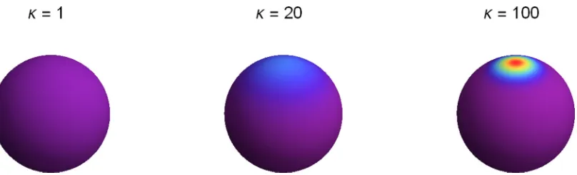
To illustrate our results, we shall pick the von Mises–Fisher distribution [41]pκ(θ)=κeκcosθ/(4πsinhκ) for our random generator ˆUn in Eq. (1). This distribution can be seen as
the counterpart of a Gaussian over the Bloch sphere: it becomes uniform for κ →0 (i.e., n is equally likely to point in any direction, as in a blackbox scenario [42,43]), whereas it localizes sharply around the z axis for κ→ ∞. In AppendicesBandC, we provide an explicit operator-sum representation for this choice ofϕ, as well as expressions for the resultantK(ϕ),FN(ϕ), andfN(ϕ).
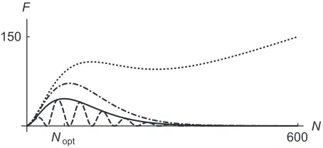
Nopt 600
N 150
[image:4.608.59.286.71.175.2]F
FIG. 2. Quantum Fisher information vsNfor the following: the N-round sequential setting with a single-qubit initial state|+(solid line), theN-round sequential setting with a passive ancilla and two-qubit initial Bell state (dot-dashed line), and the parallel-entangled setting withN-qubit initial GHZ state (dotted line). The dashed line amounts to the phase sensitivity of ˆσx, ˆσx⊗2, and ˆσ⊗
N
x in each of the
three settings, respectively. The model parameters are the same as in Fig.1. All of the quantities plotted are dimensionless.
resort to suboptimal phase-independent estimators ˆO. It is therefore particularly interesting to see how the sensitivity of accessible observables compares with the QFI. We can study, for instance, the phase sensitivity ofσxˆ =tr{σxˆ Nˆ } or, equivalently, that of m·σ for any m in the equatorial plane. Explicit formulas are provided in AppendixC, and the resultingFσˆxis plotted alongsideF
N(ϕ) in Fig.2(dashed and solid curves, respectively).
Interestingly, asNincreases, the sensitivity ofσxˆ is seen tooscillateregularly between zero and the QFI. This can be intuitively understood if one thinks of the “dynamics” of ˆNin the Bloch sphere: The maximally coherent preparation ˆ0=
|++| lies along the equator, on the Bloch sphere surface. Then, the iterative application ofϕgives rise to a trajectory which inspirals on the equatorial plane as ˆN approaches its fixed point ˆ∞= 121at the center of the sphere. This is just a combination of the unitary rotation around the zaxis and the loss of purity that results from the average in Eq. (1). The eigenstates of the SLD follow the rotation of ˆN, whereas our actual measurement basis remains fixed. As a result, the sensitivity of ˆσxoscillates between 0 andFN(ϕ), with the latter saturated when the two bases coincide (see AppendixCfor a visual description).
B. Parallel-entangled setting
As a comparison, let us now consider the parallel-entangled strategy, i.e., a single-round protocol starting from an en-tangled state of the N qubits. We will choose the max-imally entangled Greenberger-Horne-Zeilinger (GHZ) state
1 √
2(|0 ⊗N+ |
1⊗N) [44] as initial preparation. Although this may not be optimal for noisy parameter estimation [6,7,45], it comes with the advantage that it keeps a simple form under the local application of our channel on allNprobes. It also has the same degree of quantum coherence as the single-qubit|+ state, as measured by the1-norm [20]. This choice allows us to obtain an analytic expression for the QFI (see AppendixE), which is plotted in Fig.2(dotted curve) along with the QFI of the sequential case. Note that while we use the same notation N for the number of rounds in the sequential case and for the number of probes in the parallel one, these are essentially
different resources. One can nonetheless make sense of the comparison between the two metrological settings by invoking their formal equivalence in the absence of noise [19], and by recalling thatNequals the overall number of interactions with the phase-imprinting channel in both cases.
The resulting parallel QFI exhibits a linear asymptotic scaling withN 1, unlike the sequential setting. However, even if such a largeN-qubit entangled probe could be prepared, its maximum sensitivity would only be saturated by some phase-dependentcollectivemeasurement on allNprobes [18]. Indeed, in AppendixE, we show that this parallel QFI may be split into two contributions: one with a profile similar to that of the sequentialFN(ϕ), stemming from the matrix elements of the output state in the subspace of total angular momentum J2=N/2, and another one related to the complementary subspace, which depends on the phaseϕthrough the longitu-dinal deformation parameterλ(ϕ). It is precisely this second contribution which endows the probe with a linearly increasing sensitivity at largeN. It seems intuitively clear that singling out the relevant information contained in the subspaceJ2< N/2 requires a collective estimator, such as ˆJ2itself. Note that such coherent manipulations may be demanding to implement, or even unavailable in case the probes are transmitted toNremote stations during the process.
Alternatively, one could ask about the performance of a collection of accessible separable measurements, such as
ˆ σ⊗N
x , implemented locally on each probe and supplemented by classical communication in the data-analysis stage [3]. The corresponding phase sensitivity can also be computed analytically (see AppendixE), and quite remarkably it turns out tocoincidewith that of ˆσxin theN-round setting (i.e., the dashed line in Fig.2). This behavior is generic and does not de-pend on the specific suboptimal observable measured on each probe. That is, although the parallel-entangled setting can, in principle, outperform the sequential one asymptotically [37], we find that they may become metrologically equivalent when the probe readout at the output is limited to measuring local observables: This restrictionde factobanishes the asymptotic linear scaling of the precision.
It is important to remark that we assumed a particular probe preparation (GHZ states). Therefore, our observations should not be understood as a general “no-go” result, advocating against parallel-entangled estimation strategies in the presence of noise. The general question of whether the gap between sequential and parallel-entangled settings [37] persists when optimal input states and more general separable measurements are considered is definitely worthy of further investigation, although it lies beyond the scope of this paper.
C. Sequential setting with passive ancilla
Finally, as an example of the usefulness of entanglement in a practical sequential scenario, let us supplement the probe with a passive two-level ancilla. Specifically, we can prepare the probe-ancilla pair in a Bell state|± ≡ √1
2(|00 ± |11) (which has the same1-norm of coherence as the single-qubit
|+andN-qubit GHZ states) and apply the noisy channel only on the first qubit, yielding ˆN =(ϕ⊗1)N|
to the same sensitivity as the single-qubit unassisted scenario (dashed curve in Fig.2), performing instead a nonseparable (yet manageable) measurement such as ˆO= |++| −
|−−|does provide a sizable increase in phase sensitivity (see AppendixD).
V. DISCUSSION
In general, one may conclude that using independent probes in a sequential scheme, possibly supplemented by correlated passive ancillas, offers apractical advantagein noisy param-eter estimation, in spite of the potential superiority of parallel-entangled strategies [37]. As we illustrated, acquiring partial information about the geometry of the parameter-imprinting process allows one to optimize the estimation protocol at the single-probe level by simply adjusting the sampling time or number of rounds. Such a sequential estimation protocol relies on the initial amount of “unspeakable” coherence [21,22], which is a genuinely quantum feature [20], and is here con-firmed as the key resource for estimating parameters encoded in incoherent operations, which include all phase-covariant channels. However, the estimation performance only scales linearly or “classically” in the probe size, whereby scaling up the probe size is intended as repeating the optimized sequential procedureM1 times using independent probe qubits, all initialized in a maximally coherent state. Nonetheless, at the single-probe level, the sensitivity does scale quadratically in the number of roundsN, providedNis well belowNopt.
Notably, in the technologically relevant limit ofϕ1 (e.g., magnetometry in a very weak magnetic field), the optimal number of rounds Nopt stays fairly large even for relatively lowκ(see AppendixB), which translates into a very uncertain phase generator. As a result, a quadraticlike scaling of the precision for each individual probe can be maintained up to many iterations, although definitely not asymptotically. An interesting next step could be to extend our analysis to multiparameter metrology, e.g., considering the simultaneous estimation of the phaseϕ and the noise parameterκ, or the actual generator ˆHn[46].
To conclude, let us remark that, in general, the comparison between different metrological settings is a particularly tricky subject since all theresourcesmust be identified and properly accounted for [4,22,47,48]. For instance, in spite of the formal equivalence of sequential and parallel settings in the absence of noise, promoting the “number of rounds” to the status of resource at the same level as the “number of probes” is probably not fair since the actual costs of preparation, control, and measurement of an additional quantum probe are not comparable to the costs of increasing the sampling time for one additional round. It is surely worthwhile to put different metrological settings under a unified setup, also including feedback control protocols, so as to carry out an objective bookkeeping of the associated costs. This will be the subject of future work.
ACKNOWLEDGMENTS
We acknowledge the European Research Council (ERC StG GQCOP, Grant No. 637352) and the Royal Society (Grant No. IE150570) for financial support. We thank A.
Datta, R. Demkowicz-Dobrza´nski, A. Farace, C. Gogolin, M. Gut¸˘a, L. Maccone, M. Mehboudi, K. Macieszczak, K. Modi, and M. Oszmaniec for useful discussions, and especially J. Kołody´nski for helping us improve the manuscript with his feedback.
APPENDIX A: LOWER BOUND FOR THE QFI OF A UNITAL PHASE-COVARIANT CHANNEL
Below we will give further details about the tight-fitting lower boundfN(ϕ) to the QFIFN(ϕ). As stated in the main text, maxˆˆ|(∂ϕKN)†∂ϕKN|ˆFN(ϕ) [38,39] does hold in general, although it is not necessarily a tight bound. If the maximization were not restricted to vectorized physical states |ˆ, but extended to all normalized four-dimensional vectors in Liouville space, we would end up calculating the op-erator norm||(∂ϕKN
)†∂ϕKN||
maxˆˆ|(∂ϕKN)†∂ϕKN|ˆ. This equals the largest eigenvalue of the enclosed matrix. In particular, for the family of channels considered in the main text and represented by K(ϕ), the eigenvalues of (∂ϕKN
)†∂ϕKN
areη1=0,η2=N2λ2N−2(∂ϕλ)2, andη3,4= N2λ2⊥N−2[(∂ϕλ⊥)2+λ2⊥(∂ϕg)2], which is doubly degenerate.
Now, considering the expression given in the main text for the QFI of any phase-covariant unital channel and recalling that 0< λ⊥<1, one can readily see that η3,4≡fN(ϕ) FN(ϕ). Furthermore, wheneverη2< η3,4, one could elegantly lower-bound the channel QFI as||(∂ϕKN)†∂ϕKN|| =fN(ϕ) FN(ϕ). This is the case, for instance, in the example considered in the main text, based on the von Mises–Fisher distribution. In the most general case,fN(ϕ) still remains a close-fitting lower bound to the QFI for the whole class of channels represented byK(ϕ).
APPENDIX B: OPERATOR-SUM REPRESENTATION OF THE NOISY PHASE-IMPRINTING CHANNEL In this section, we shall give explicit expressions for a set of Kraus operators{Kiˆ }realizing the noisy phase-imprinting channelϕˆ =iKiˆ ˆKiˆ†in Eq. (1) of the main text, when the generic distributionp(θ,φ) for the random generator ˆHn
is chosen to be the von Mises–Fisher distribution (vMF) distributionpκ(θ). Recall from the main text thatpκ(θ) reads
pκ(θ)= κe κcosθ
4πsinhκ, (B1)
where the concentration parameterκ0 gives an idea of how narrow the distribution ofnis around thezaxis. Forκ →0, the vMF distribution is uniform on the Bloch sphere, while it increases in concentration for greaterκ. This is illustrated in Fig.3.
The Kraus operators {Kiˆ }may be readily obtained from the eigenvalues and eigenvectors of the corresponding Choi matrix of the map C. This is the matrix resulting from (ϕ⊗1)|++|, where |+ is the two-qubit Bell state
|+ ≡ √1
FIG. 3. Visualization of the vMF distribution for varyingκ. The probability density runs from indigo at its lowest to red at its highest. Note that the settingκ=1, used to generate the illustrations of the main text, actually corresponds to a very broad distribution for the random generator ˆHn. All of the quantities plotted are dimensionless.
matrix elements of the corresponding Kraus operatorsKi,kl≡ k|Kiˆ |l(withi∈ {1, . . . ,4}andk,l∈ {1,0}) are
K1,10=K2,01=
√
2 sinϕ κ
√
κcothκ−1,
K3,11= 1 2√2κ(
√
2A+B+√2A−B),
K4,11= 1 2√2κ(
√
2A+B−√2A−B),
K3,00=
C √
2K3,11, K4,00 = −
C √
2K4,11,
(B2)
whereA(∈R),B(∈R), andC(∈C) are the following functions ofκandϕ:
A=1+κ2−cos 2ϕ−2κsin2ϕ cothκ,
B=
2κ2(cosh 2κ−2κ2−1) csch2κ sin22ϕ,
C=
κ2sin22ϕ(1+2κ2−cosh 2κ)+2[(1+κ2−cos 2ϕ) sinhκ−2κcoshκsin2ϕ]2 κ[κsinh (κ+2iϕ)−cosh (κ+2iϕ)+coshκ]−2 sin2ϕsinhκ .
(B3)
This operator-sum representation then allows simple calculation ofϕˆ by bypassing the difficult integration that defines the channel.
The Liouville representationK(ϕ) of the channelϕtakes the form
K(ϕ)=
⎛ ⎜ ⎜ ⎝
|K3,00|2+ |K4,00|2 0 0 K22,01 0 K3,00K3,11+K4,00K4,11 0 0 0 0 K3∗,00K3,11+K4∗,11K4,11 0 K2
1,10 0 0 K32,11+K42,11
⎞ ⎟ ⎟
⎠, (B4)
in terms of the operator-sum representation of the channel. In particular, we have that
λ=1−2K22,01, λ⊥= |S|, and g= −arg(S), (B5)
where S= √
4A2−B2
2√2κ2 C(∈C) and arg(S) denotes the complex
argument ofS.
APPENDIX C: PHASE SENSITIVITY IN THE SEQUENTIAL SETTING
1. Quantum Fisher information
We will now provide a closed formula for the QFIFN(ϕ) for a single two-level probe undergoingNsequential applications ofϕ. We shall take the optimal “plus” state|+ = √1
2(|0 +
|1) as the probe preparation ˆ0.
Recall from the main text thatFN(ϕ) of ˆNis simply written as
FN(ϕ)=4 i,j
qi (qi+qj)2
ψi|∂ϕNˆ |ψj2, (C1)
whereqiand|ψiare the eigenvalues and eigenvectors of ˆN, and any terms for whichqi+qj =0 are excluded from the sum. The output state of the probe ˆN =Nϕ|++|can be obtained by repeatedly applying the Kraus operators defined in Eqs. (B2) and (B3). After a lengthy calculation, one may castFN(ϕ) in compact form as
FN(ϕ)=N2|S|2NS S
21− |S1|2− |NsinS|22(Nν−μ), (C2)
FIG. 4. Contour plot of the optimal number of iterationsNoptas
obtained from the maximization offN(ϕ), as a function of the phase
ϕand the concentration parameterκ. All of the quantities plotted are dimensionless.
the QFI of Eq. (C2) does grow asN2before a peak is reached at some optimalNopt, after which there is a noise-dependent exponential decay, asymptotically approaching zero in the limit of largeN.
2. Lower bound on the quantum Fisher information We will now comment on the expression of the lower bound fN(ϕ) on the QFI for our particular noisy channel, in the sequential setting. In this particular case, fN(ϕ)= N2λ2N−2
⊥ [(∂ϕλ⊥)2+λ2⊥(∂ϕg)2]=N2|S|2N|S/S|2. Note that fN(ϕ) is thus just the prefactor in the expression for FN(ϕ) in Eq. (C2), which essentially modulates the amplitude of the optimal phase sensitivity.
In Fig. 4, we plot Nopt= −1/ln|S| as a function of the concentration parameter κ and the phase ϕ. Note that forϕ small enough, the optimal number of applications remains on the order of 103 even for very low κ (i.e., quasiuniform distribution for the rotation axisn). As a result, the sequential setting may exhibit a superclassical scaling in the sensitivity, up to a significantly large number of rounds.
3. Phase sensitivity of ˆσx
The maximum phase sensitivity, given by the QFI, may only be reached when an optimal estimator is measured on the out-put state of the probe. Recall that such optimal estimator must be diagonal in the eigenbasis of the SLD ˆL, which reads [31]
ˆ
L=2 ij
ψi|∂ϕˆN|ψj qi+qj
|ψiψj|. (C3)
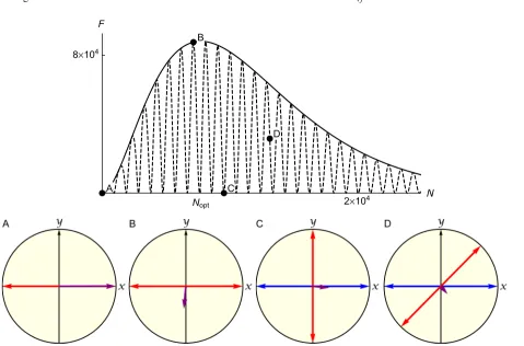
A
B
C
D
Nopt 2×10⁴ N
F
8×10⁴
FIG. 5. Top: QFI (solid line) and phase sensitivity of ˆσx(dashed line) forϕ=0.01 andκ=0.5. Representations of the evolved probe state
(purple arrow), optimal measurement basis (red arrow), and suboptimal measurement basis (blue arrow) as Bloch vectors on the equatorial plane are shown in the bottom panels. (A) Initially, the probe state and both measurements are aligned. (B) The phase sensitivity of ˆσx meets
the QFI when the measurement bases realign. (C) The phase sensitivity of ˆσxvanishes whenever the measurement bases become perpendicular.
(D) Otherwise, the phase sensitivity of ˆσx oscillates between zero and the QFI. Note that as N grows, the optimal basis vectors become
[image:7.608.71.550.356.672.2]We can instead calculate the phase sensitivity FOˆ of some suboptimal observable ˆOdefined as in Eq. (4). Choosing ˆσx as our estimator yields
Fσˆx =N2|S|2NS
S
21cos− |2[νS|+2N(N−1)μ]
cos2(N μ). (C4)
The QFI and the phase sensitivityFσˆxare depicted in Fig.5
for particular values of ϕ andκ. It can be seen that FN(ϕ) displays the aforementioned quadratic behavior followed by an exponential tail-off, whereasFσˆx oscillates between zero and
FN(ϕ). This curious behavior can be understood by visualizing the evolved probe state ˆN and the measurement eigenbases of both the SLD ˆLand the suboptimal estimator ˆσx on the equatorial plane of the Bloch sphere [see Figs.5(a)–5(d)].
Here, the initial probe state ˆ0= |++|begins on thex axis at the surface of the sphere. As stated in the main text, the Bloch vector of the evolved state ˆNinspiralstowards the normalized identity. This is a result of the rotation around the zaxis due to the parameter-encoding unitary, and the loss of purity due to the noise. The optimal measurement basis begins on thexaxis, parallel to the probe state, and rotates withN. Meanwhile, the fixed measurement basis lies on thex axis, so that it periodically coincides with the optimal one: when they are parallel, Fσˆx =F
N(ϕ), whereas when they become perpendicular,Fσˆx =0. The frequency of these oscillations is
given approximately by|μ|/π.
APPENDIX D: PHASE SENSITIVITY IN THE SEQUENTIAL SETTING WITH A PASSIVE ANCILLA In this section, we will give further details about the performance of the sequential estimation setting when the probe is supplemented with a passive two-level ancilla. Recall from the main text that in this case, we prepare the two qubits in a Bell state |± = √1
2(|00 ± |11) and proceed to apply sequentiallyNtimes the phase-imprinting channel as
ˆ
N=(ϕ⊗1)N|±±|.
The resulting “evolved” two-qubit state has maximally mixed marginals at anyN. The corresponding QFIFN(anc)(ϕ) may be readily evaluated to
FN(anc)(ϕ)
= 1
4N 2
D++D−+8λ 2N ⊥ (∂ϕg)2 1+λN
+2λ
2(N−1) (∂ϕλ)2
1−λN
,
(D1)
where
D±≡ |
2λN⊥−1(∂ϕλ⊥)±λN−1(∂ϕλ)|2 1±2λN
⊥+λN
. (D2)
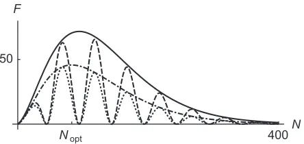
Nopt 400N
[image:8.608.325.547.70.175.2]50 F
FIG. 6. QFI for the sequential setting when the probe is supple-mented with a passive ancilla (solid) as a function of the number of applications of the channelN. The QFI for a single two-level probe (without ancilla) is included for comparison (dot-dashed line). The phase sensitivity of ˆσx⊗σˆx(dotted line) and ˆO≡ |++| − |−−|(dashed line) have also been plotted. The vMF distribution is assumed for the stochastic generator of the phase rotations, with ϕ=0.1 andκ=1. All of the quantities plotted are dimensionless.
Once again, we shall particularize our results choosing the vMF distribution for the stochastic generator (see Fig.6). In the first place, note that FN(anc)(ϕ) notably outperforms the sensitivity of a single probe. In particular, when a separable estimator such as ˆσx⊗σxˆ is considered, the phase sensitivity of the probe-ancilla pair remains upper-bounded by the QFI of a single probe. However, as we can see, when a Bell measurement is performedjointlyon the probe and the ancilla, the ensuing sensitivity can come much closer to the ultimate limit set byFN(anc)(ϕ).
APPENDIX E: PHASE SENSITIVITY IN THE PARALLEL SETTING
1. Quantum Fisher information
We will now compute the QFI in the parallel setting for a maximally entangled Greenberger-Horne-Zeilinger (GHZ) state of the N probes, |GHZ ≡ √1
2(|0
⊗N+ |1⊗N). The
output state ˆN =⊗ϕN|GHZGHZ| is a type of X state, that is, a state represented by a 2N×2N matrix with nonzero elements ˆN,mn= m|Nˆ |n (withm,n∈ {0,1, . . . ,2N−1}) only along the main diagonal and in the extreme off-diagonal corners. In particular, we find
ρN,mm=αN−H(m)(1−α)H(m)+αH(m)(1−α)N−H(m),
ρN,0(2N−1)=SN, (E1)
ρN,(2N−1)0=S¯N,
where H(m) is the Hamming weight ofm, i.e., the number of 1’s in the binary representation ofm. The overbar denotes complex conjugation andαis given by
α= 1
2(1−λ)=
2(−1+κcothκ) sin2ϕ
Then, the QFI (FNpar) may be calculated using Eq. (C1) and is given by
FNpar = N 2
8
⎛ ⎜ ⎝−8|S|
2NS S
2sin2(ν−μ) (1−α)N+αN
+
2|S|NSSsin(ν−μ)+4[(1−α)N−1α−αN] cotϕ2 (1−α)N+αN− |S|N +
2|S|NSSsin(ν−μ)−4[(1−α)N−1α−αN] cotϕ2 (1−α)N+αN+ |S|N
+2 N−1
k=1
N k
[k+N(α−1)](1
α−1) k
αN
α−1 +(1−α) N−1−kαk
(k−N α)2cot2ϕ
1
α −1
k
αN+(1−α)N−kαk
. (E3)
The contribution of the first term in Eq. (E3) to the total sensitivity is qualitatively similar to the QFI in the sequential setting, i.e., it scales quadratically for low N and, after peaking, it decays exponentially to zero. However, the second term contributes with an classical-like increase inN, which ultimately yields a linear asymptotic scaling for the overall QFI. As stated in the main text, while the first contribution relates to the outermost “corners” of the density operator (i.e., the subspace spanned by|00· · ·0 and|11· · ·1, with total angular momentumJ =1/2), the second one is determined by all of the matrix elements along the diagonal of the state, such that J <1/2. In particular, accessing all of the relevant information giving rise to the classical-like asymptotic scaling of the sensitivity, requires therefore one to perform a nonseparable measurement capable of differentiating the subspaceJ =1/2 from its complementaryJ <1/2, such as a measurement of the total angular momentum ˆJ2.
2. Phase sensitivity of ˆσ⊗N x
Analogously to the sequential setting, one can consider the sensitivity of a suboptimal estimator. In particular, we can compute the phase sensitivity of the separable observable
ˆ O=σˆ⊗N
x by resorting to Eqs. (4) and (E1). As pointed out in the main text, this yields exactly the same formula as Eq. (C4), thus implying that the parallel-entangled and unentangled sequential settings are metrologically equivalent as long as the estimation is constrained to separable measurements.
Note, furthermore, that in both sequential and parallel settings, one could consider alternative observables to ˆσx with eigenbases on the equatorial plane of the Bloch sphere, such as ˆσy or even some suboptimal yet phase-dependent observable. Generically, the oscillatory behavior will remain, but the periodicity and locations of the maxima will change depending on the chosen observable.
[1] B. P. Abbottet al.(LIGO Scientific Collaboration and Virgo Collaboration),Phys. Rev. Lett.116,061102(2016).
[2] V. Giovannetti, S. Lloyd, and L. Maccone,Science306,1330
(2004).
[3] V. Giovannetti, S. Lloyd, and L. Maccone,Phys. Rev. Lett.96,
010401(2006).
[4] V. Giovannetti, S. Lloyd, and L. Maccone,Nat. Photon.5,222
(2011).
[5] R. Demkowicz-Dobrza´nski, J. Kołody´nski, and M. Gut¸˘a,Nat. Commun.3,1063(2012).
[6] S. F. Huelga, C. Macchiavello, T. Pellizzari, A. K. Ekert, M. B. Plenio, and J. I. Cirac,Phys. Rev. Lett.79,3865(1997). [7] B. Escher, R. de Matos Filho, and L. Davidovich,Nat. Phys.7,
406(2011).
[8] Y. Matsuzaki, S. C. Benjamin, and J. Fitzsimons,Phys. Rev. A 84,012103(2011).
[9] A. W. Chin, S. F. Huelga, and M. B. Plenio,Phys. Rev. Lett. 109,233601(2012).
[10] K. Macieszczak,Phys. Rev. A92,010102(2015).
[11] A. Smirne, J. Kołody´nski, S. F. Huelga, and R. Demkowicz-Dobrza´nski,Phys. Rev. Lett.116,120801(2016).
[12] T. Tanaka, P. Knott, Y. Matsuzaki, S. Dooley, H. Yamaguchi, W. J. Munro, and S. Saito,Phys. Rev. Lett.115,170801(2015). [13] R. Chaves, J. B. Brask, M. Markiewicz, J. Kołody´nski, and A.
Ac´ın,Phys. Rev. Lett.111,120401(2013).
[14] J. B. Brask, R. Chaves, and J. Kołody´nski, Phys. Rev. X 5,
031010(2015).
[15] E. M. Kessler, I. Lovchinsky, A. O. Sushkov, and M. D. Lukin,
Phys. Rev. Lett.112,150802(2014).
[16] W. D¨ur, M. Skotiniotis, F. Fr¨owis, and B. Kraus,Phys. Rev. Lett. 112,080801(2014).
[17] T. Monz, P. Schindler, J. T. Barreiro, M. Chwalla, D. Nigg, W. A. Coish, M. Harlander, W. H¨ansel, M. Hennrich, and R. Blatt,Phys. Rev. Lett.106,130506(2011).
[18] K. Micadei, D. A. Rowlands, F. A. Pollock, L. C. C´eleri, R. M. Serra, and K. Modi,New J. Phys.17,023057(2015).
[19] L. Maccone,Phys. Rev. A88,042109(2013).
[20] T. Baumgratz, M. Cramer, and M. B. Plenio,Phys. Rev. Lett. 113,140401(2014).
[21] I. Marvian and R. W. Spekkens, Nat. Commun. 5, 3821
(2014).
[22] I. Marvian and R. W. Spekkens,arXiv:1602.08049.
[23] C. Napoli, T. R. Bromley, M. Cianciaruso, M. Piani, N. Johnston, and G. Adesso,Phys. Rev. Lett.116,150502(2016).
[24] B. L. Higgins, D. W. Berry, S. D. Bartlett, H. M. Wiseman, and G. J. Pryde,Nature (London)450,393(2007).
[25] A. S. Holevo,Probabilistic and Statistical Aspects of Quantum Theory, 1st ed. (Edizioni della Normale, Pisa, 2011).
[27] M. A. Nielsen and I. L. Chuang,Quantum Computation and Quantum Information(Cambridge University Press, Cambridge, 2000).
[28] I. Bengtsson and K. Zyczkowski,Geometry of Quantum States: An Introduction to Quantum Entanglement(Cambridge Univer-sity Press, Cambridge, 2006).
[29] D. Braun, O. Giraud, I. Nechita et al.,J. Phys. A47,135302
(2014).
[30] S. L. Braunstein and C. M. Caves,Phys. Rev. Lett.72,3439
(1994).
[31] O. Barndorff-Nielsen and R. Gill,J. Phys. A33,4481(2000). [32] R. D. Gill and B. Y. Levit,Bernoulli1,59(1995).
[33] M. Tsang,Phys. Rev. Lett.108,230401(2012).
[34] P. Sekatski, M. Skotiniotis, J. Kołody´nski, and W. D¨ur,
arXiv:1603.08944.
[35] M. G. A. Paris,Int. J. Quantum Inf.7,125(2009).
[36] L. Jing, J. Xiao-Xing, Z. Wei, and W. Xiao-Guang,Commun. Theor. Phys.61,115(2014).
[37] R. Demkowicz-Dobrza´nski and L. Maccone, Phys. Rev. Lett. 113,250801(2014).
[38] R. Yousefjani, S. Salimi, and A. Khorashad,arXiv:1602.01691. [39] S. Alipour, M. Mehboudi, and A. T. Rezakhani,Phys. Rev. Lett.
112,120405(2014).
[40] M. Karpi´nski, C. Radzewicz, and K. Banaszek,JOSA B25,668
(2008).
[41] R. Fisher,Proc. R. Soc. Lond. A217,295(1953).
[42] D. Girolami, A. M. Souza, V. Giovannetti, T. Tufarelli, J. G. Filgueiras, R. S. Sarthour, D. O. Soares-Pinto, I. S. Oliveira, and G. Adesso, Phys. Rev. Lett. 112, 210401
(2014).
[43] A. Farace, A. De Pasquale, G. Adesso, and V. Giovannetti,New J. Phys.18,013049(2016).
[44] D. M. Greenberger, M. A. Horne, and A. Zeilinger, inBell’s Theorem, Quantum Theory and Conceptions of the Universe, edited by M. Kafatos, Vol. 37 (Springer, Netherlands, 1989), pp. 69–72.
[45] M. Jarzyna and R. Demkowicz-Dobrza´nski,Phys. Rev. Lett. 110,240405(2013).
[46] T. Baumgratz and A. Datta, Phys. Rev. Lett. 116, 030801
(2016).
[47] M. Zwierz, C. A. P´erez-Delgado, and P. Kok,Phys. Rev. Lett. 105,180402(2010).
[48] L. del Rio, L. Kraemer, and R. Renner,arXiv:1511.08818. [49] H. Breuer and F. Petruccione, The Theory of Open