Development of an adaptive discharge coefficient to improve the accuracy of crossventilation airflow calculation in building energy simulation tools

1

Development of an Adaptive Discharge Coefficient to Improve the Accuracy of Cross-ventilation Airflow Calculation in Building Energy Simulation Tools

Mohammadreza Shirzadia_{, Parham A. Mirzaei}b_{, Mohammad Naghashzadegan}a,1

a _{Mechanical Engineering Department, University of Guilan, Rasht, Iran}

b _{Architecture and Built Environment Department, University of Nottingham, Nottingham, UK}

Abstract

Airflow network (AFN) model embedded in building energy simulation (BES) tools such as EnergyPlus is extensively used for prediction of cross-ventilation in buildings. The noticeable uncertainty in the measurement of the surface pressure, discharge coefficient, and simplifications applied to the orifice-based equation result in considerable discrepancies in the prediction of the cross-ventilation airflow rate values. Computational Fluid Dynamics (CFD) provides more accurate results comparing to the orifice-based equations although with an excessive computational cost.

The aim of this study is, therefore, to improve the accuracy of the orifice-based model by development of an adaptive correlation for the discharge coefficient using CFD. Hence, a validated CFD model for the cross-ventilation of an unsheltered building is firstly developed using an experimental study. In the next step, by exploiting Latin hypercube sampling (LHS) approaches, a large CFD dataset of 750 scenarios for different building geometries (i.e. square cube, cuboid and long corridor) is generated; the dataset is then coupled to the AFN cross-ventilation model to obtain an adaptive correlation for the discharge coefficient as a function of the openings’ geometries and location using response surface (RSM) and radial basis function (RBF) models.

Results show that the newly developed adaptive correlation successfully increases the accuracy of AFN model for the cross-ventilation modeling of unsheltered buildings as the relative errors for the airflow rate prediction of different building geometries are significantly decreased up to 28% in comparison with the cases with constant discharge coefficient and surface-averaged and local-surface wind pressure coefficients. Results, also demonstrate the importance of considering the value of the local-surface wind pressure in the AFN model for the square cube and cuboid building models.

Keywords: Cross-ventilation, CFD, Sampling, Discharge coefficient, Building Energy Simulation, Correlation

1 _{Corresponding author: Khalij Fars highway, Rasht, Iran}

2 Nomenclature

𝜌 Density 𝑈_𝐻 Inflow mean streamwise velocity at building

height 𝐻

𝑡 Time 𝐻 Building height

𝑥, 𝑦, 𝑧 Component of space coordinate 𝛼 Power-law exponent 𝑈𝑖 Component of mean velocity

vector

𝑁 Number of data points

𝑆_𝑀𝑖 Momentum source 𝑂_𝑖 Observed value

𝑘 Turbulent kinetic energy 𝑃_𝑖 Predicted value

𝜇𝑙 Molecular viscosity 𝐹𝐴𝐶2 Fraction of the predictions within a factor of 2 of the observations

𝐶_𝜇 Turbulence model constant 𝑁𝑀𝑆𝐸 Normalized mean square error

𝜀 Turbulent dissipation rate 𝑢_𝑖 Fluctuating velocity component in turbulent flow

𝐷 Building depth 𝐶𝑝 Pressure coefficient

𝑃 pressure 𝐶_𝑑 Discharge coefficient

𝑊 Building width 𝐶_𝑑∗ Adaptive discharge coefficient

𝑄 Airflow rate 𝑔 Acceleration of gravity

𝐴𝑜 Opening area 𝜃 Opening area reduction factor

Z Vertical coordinate

1.

Introduction

In developed and developing countries building sector accounts for about 40% of total energy demand in cities [1, 2]. The potential of natural and wind-driven ventilation for energy saving [3, 4] and thermal comfort [5, 6] has been recognized as an effective strategy in modern and traditional buildings [7]. Natural ventilation has a complex mechanism [8], placing it in the subject of many studies during the past 50 years [9]. Wind-driven cross-ventilation is the most commonly type of the natural ventilation in which pressure difference across the building caused by wind imposes the airflow thorough the building openings [10].

Researches are mainly focused to understand the complex mechanism of the cross-ventilation [11-13], to develop theoretical and empirical models [14-16], and to provide details of the airflow parameters [17-21]. Wind tunnel measurement [22-24] and on-site measurement [25-27] are broadly employed to explore the mechanism of the cross-ventilation, but their applications are mainly limited to simplified building geometries. Analytical models and computational fluid dynamics (CFD) method, on the other hand, are relatively cheaper and easier to provide the cross-ventilation information in complex building geometries.

3

this model, in contrast to the simplified orifice model, which is based on Bernoulli equation, the dynamic pressure of the jet is considered in an energy balance equation. The total pressure loss and mass flow rate through openings are correlated to each other in the power loss equation. Another model for evaluation of the cross-ventilation is the local dynamic similarity model (LDSM) introduced by Kurabuchi et al. [15]. This model is developed based on a fact that the cross-ventilation flow structure in the vicinity of an inflow opening creates dynamic similarity under the condition that the ratio of the cross-ventilation driving pressure to the dynamic pressure of the cross flow is consistent at the opening. They used a Large Eddy Simulation (LES) model to estimate the variation of pressure along the stream tube, crossing the openings of a model building, and introduced a non-dimensional pressure, which is a function of openings’ position and wind direction. Using this developed model, they calculated the discharge coefficient of the building model opening for different wind angles and opening positions.

Eventually, airflow network model (AFN) [29] is developed based on the mass balance and Bernoulli’s equation between different nodes connected via airflow components (linkage) such as windows and doors. In this model, the variable defined at each node is pressure while the linkage variable is the mass flow rate [30]. Even though the power balance and LDSM models provide more accurate results and also present detailed information of the fluid dynamics, these models never gain the popularity of simplified orifice-based models such as AFN. The simplified formulation of the orifice-based models makes them a good choice for integrating with the building energy models for realistic engineering applications. Furthermore, there are many resources in open literature regarding the input parameters to the orifice-based models which make their application easy although their accuracy for large openings remains a controversial issue.

The orifice equation for the airflow rate (𝑄) through a sharp-edged opening, which is used in AFN model, can be expressed as below:

𝑄 = 𝑐_𝑑𝐴√2∆𝑃

𝜌 (1)

where 𝑐𝑑, 𝐴, and 𝜌 are the discharge coefficient, opening area and air density, respectively. The value of pressure difference ∆𝑃 across the opening is usually expressed in the form of pressure coefficient:

𝑐𝑃 =

𝑃 − 𝑃_𝑜 1 2 𝜌𝑈𝑟𝑒𝑓2

(2)

4

opening. Results of the numerical and experimental studies show that these assumptions are not fully satisfied for the cross-ventilation in buildings. For instance, according to the works presented in [12, 13, 21, 32], not only does the kinetic energy of the entering jet penetrate inside the building, but also a noticeable amount of the kinetic energy can exit across the outlet opening.

In addition to the inaccuracy of the orifice-based models for the large openings due to the idealized Bernoulli’s equation, there are other sources of discrepancy in these models such as the one associated with the input parameters as addressed in [33-38]. The input parameters (e.g. the discharge and pressure coefficients in addition to the velocity profile), according to Karava et al. [31], are coupled together and their interaction should be analyzed in detail for a suitable cross-ventilation design. These parameters depend on many factors, including the building and opening geometries, and the sheltering effect of the surrounding buildings [31].

As highlighted in [39], assuming a constant value for 𝐶_𝑑 can be a major source of error in the AFN model in cross-ventilation studies. The value of discharge coefficient is a function of different parameters, including the opening porosity and Reynolds (𝑅𝑒) number [31, 39], wind direction [40, 41], turbulence parameters [42], pressure difference across the openings [43], and building geometry. A variation of 𝑐_𝑑 was reported for a gable roof-sloped building model to vary from 0.74 to 0.9 and 0.6 to 0.71 for velocity ratios of 0.63 and 0.5 [31]. The variation of 𝑐_𝑑 was reported to be insignificant for the wind incidence angles less than 30 degrees, but its value was shown to drop rapidly to a minimum value of 0.1 for the wind incident angles between 30 and 90 degrees [43].

Pressure coefficient 𝐶_𝑃 is another input parameter for the orifice-based model, which is generally obtained by wind tunnel/full-scale measurements, and analytical correlations. 𝑐_𝑃 values obtained from the measurement datasets [44, 45] and analytical methods [46-48] are only available for some limited basic building shapes. A noticeable difference between 𝐶_𝑃 values obtained from different datasets is reported, especially when the local distribution of 𝑐𝑃 and sheltering effect are taken into the account [34]. The high importance of considering the uncertainties in the wind-induced pressure coefficient is widely emphasized [38] and recognized to be related to the existence of a wide range of affecting parameters, including façade design specification, building geometry, opening position, sheltering effect by surrounding buildings, obstacles (e.g. trees), and stochastic wind characteristics (i.e. direction, speed, turbulence intensity) [49].

5

defined in this study, which is a function of the openings’ geometry and location. The proposed framework for the accuracy improvement of the orifice-based model is described at first, and then details of the CFD simulation setup, validation and utilized experimental measurements are provided. A database is then generated from a series of CFD simulations using the Latin hypercube sampling methods while the modified discharge coefficient of the orifice-based model is adapted from the generated database using meta-model approximations. Finally, the accuracy of the proposed methodology is discussed by comparing the results of the orifice-based model, which utilizes the adaptive discharge coefficient, with the CFD and experimental measurements for different openings configurations.

2.

Methodology

2.1 Proposed Framework

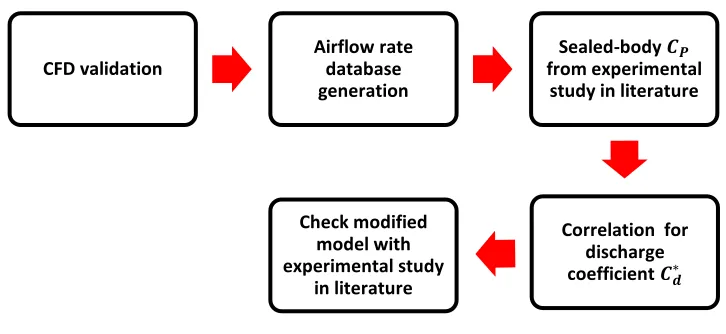
The proposed methodology for the accuracy improvement of the orifice-based model is shown in Figure 1. The goal is to generate an adaptive correlation for the discharge coefficient (𝐶_𝑑) as a function of building geometry, and openings’ dimension and position. Therefore, at the first step, a validated CFD model for the cross-ventilation through an isolated building with two openings on the opposite walls was developed based on an experimental measurement conducted by Tominaga and Blocken [13]. In the next step, a database for the airflow rate of the building model was generated using the validated CFD model setting by alteration of the building and openings geometrical parameters shown in Figure 2; the optimal Latin hypercube sampling technique [50], a modified model of the Latin hypercube sampling, was then used to generate the required population in this study.

Figure 1 Procedure for development of the new correlation for the discharge coefficient

Once the database generation was completed, the airflow rate of each design case was passed into the orifice-based model. In addition, the local-surface wind pressure coefficient at the windward and leeward openings were obtained from a series of boundary layer wind tunnel

CFD validation

Airflow rate database generation

Sealed-body 𝑪𝑷 from experimental

study in literature

Correlation for discharge coefficient 𝑪_𝒅∗ Check modified

model with experimental study

6

measurements deployed by Tamura [51]. Using the airflow rate from CFD and local surface wind pressure coefficient from the experiment, a new correlation for the discharge coefficient (𝐶_𝑑∗) was obtained as a function of the building geometry, and openings’ dimension and location. The value of the modified discharge coefficient, assuming to be equal for the windward and leeward opening, is defined as follows:

𝐶_𝑑∗ ₌ 𝑄𝐶𝐹𝐷

𝑈_𝑟𝑒𝑓𝐴_𝑜1√𝐶_𝑃1𝐸𝑥𝑝− 𝐶_𝑃𝑖

(3)

𝐶_𝑃𝑖= 𝐶𝑃1

𝐸𝑥𝑝₊₍𝐴_𝑜2 𝐴_𝑜1)

2 𝐶_𝑃2𝐸𝑥𝑝

1 +(𝐴𝑜2 𝐴𝑜1)

2 (4)

where 𝑄_𝐶𝐹𝐷 is the airflow rate predicted by CFD model while 𝑈_𝑟𝑒𝑓, 𝐴_𝑜1, and 𝐴_𝑜2 are the free-stream velocity at a reference height and area of the windward and leeward openings,

respectively. 𝐶_𝑃1𝐸𝑥𝑝 and 𝐶_𝑃2𝐸𝑥𝑝 are respectively the local-surface wind pressure coefficients at the windward and leeward openings obtained from the sealed-body measurement, and 𝐶𝑃𝑖 is the internal pressure coefficient. The calculated modified discharge coefficient of each database sample was then used to create a meta-model approximation for 𝐶_𝑑∗ using response surface (RSM) and radial basis function (RBF) models. Finally, the accuracy of the orifice-based model with the modified discharge coefficient was examined by comparing the results with an available experimental study in literature.

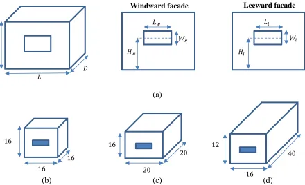
(a)

(b) (c) (d)

Figure 2 (a) Building geometry parameters for database generation. Dimensions of (b) square cube, (c) cuboid, and (d) long corridor building models

𝐿 𝐷

𝐻

𝐻𝑤

𝐿𝑤

𝑊𝑤

𝐻𝑙

𝐿𝑙

𝑊𝑙

Windward facade Leeward facade

16

16

16

16

20

20 12

16

7 2.2 Database Generation

A schematic of the automatic database generation process for the cross-ventilation model is shown in Figure 3. The Statistics and Machine Learning Toolbox™ of MATLAB was used to generate design of experiments (DOE) samples. The geometry of the building (𝐿, 𝐷, 𝐻), and the windward and leeward openings dimensions (𝐿_𝑤, 𝐿_𝑙, 𝑊_𝑤, 𝑊_𝑙) in addition to their vertical positions (𝐻_𝑤, 𝐻_𝑙) were passed to ANSYS DesignModeler in which a parametric geometrical model was created. The geometry of the building model was carried out to the ICEM CFD meshing package where a predefined mesh template was automatically applied. The created mesh was then handled in the CFX solver. After reaching an acceptable convergence, all output data, including airflow rate (𝑄) and parameters such as the opening Reynolds number (𝑅𝑒_𝑜), opening velocity ratio (𝑉_𝑟) and flow Reynolds number, were automatically calculated and linked to MATLAB software. After the completion of the process, a meta-model was generated in MATLAB to produce a new adaptive discharge coefficient (𝐶_𝑑∗). Finally, the performance of the evolved meta-model was analyzed using a cross-validation method. Simulations were conducted using an 8-core AMD® CPU processor which took about 36 hours for each building geometry.

Figure 3 A schematic of the automatic database generation for cross-ventilation models

Three different building configurations were considered in this study adapted from the literature where experimental data were available, representing 1:100 scale models of buildings with full-scale dimensions of 𝐿 × 𝐷 × 𝐻 = 16 × 16 × 16 𝑚3, 𝐿 × 𝐷 × 𝐻 = 20 × 20 × 16 𝑚3_{, and 𝐿 × 𝐷 × 𝐻 = 16 × 40 × 12 𝑚}3_{. As shown in Figure 2, the first building} model is a square cube while the second and third models are cuboids. The third building has a large depth to breath ratio of 5:2, which represents a long corridor cross-ventilation scenario. The considered range for the opening dimensions and position are shown in Table 1. The wall porosity (𝑃_𝑟) variation for windward and leeward openings is in the range of 3% ≤ 𝑃𝑟 ≤ 25% for all building models; in this range, the accuracy of the orifice-based model

CFX

Pre-processsing Run CFX solver Post-processing ICEM CFD

Paramertic mesh model Mesh generation ANSYS DesignModeler

Geometry parameterization Geoemtry creation

Airflow parameters

MATLA

B

DOE

RS

M

/R

BF

N

e

w

d

is

ch

ar

ge

c

o

e

ffi

cie

n

t

Geometric parameters

𝐻𝑤, 𝐻𝑙, 𝐿𝑤, 𝐿𝑙

𝑊𝑤, 𝑊𝑤, 𝐷, 𝐻, 𝐿

𝑄, 𝑅𝑒𝑜

8

found to be reasonable. The minimum distance between the openings and floor/roof edges is 0.1𝐻; both openings have equal distances from the side walls.

Table 1 Range of the openings dimensions for the database generation

Square cube Cuboid Long corridor

Opening length 𝐿𝑚𝑖𝑛 = 3.75

𝐿_𝑚𝑎𝑥 = 12 𝐿𝐿_𝑚𝑎𝑥𝑚𝑖𝑛= 16= 5 𝐿𝐿𝑚𝑖𝑛_𝑚𝑎𝑥= 3.75= 12

Opening width 𝑊𝑚𝑖𝑛= 1.94

𝑊_𝑚𝑎𝑥 = 6.12 𝑊𝑊_𝑚𝑎𝑥𝑚𝑖𝑛= 1.94= 6.12 𝑊𝑊𝑚𝑖𝑛_𝑚𝑎𝑥= 1.45= 4.6

Opening height 𝐻𝑚𝑖𝑛 = 0.1𝐻

𝐻_𝑚𝑎𝑥 = 0.9𝐻 − 𝑊_𝑚𝑎𝑥 𝐻_𝑚𝑎𝑥𝐻𝑚𝑖𝑛= 0.9𝐻 − 𝑊= 0.1𝐻_𝑚𝑎𝑥 𝐻_𝑚𝑎𝑥𝐻𝑚𝑖𝑛= 0.9𝐻 − 𝑊= 0.1𝐻_𝑚𝑎𝑥

2.3 Design of the Computational Experiments

The accuracy of a meta-model is directly linked to the design of computational experiments or sampling methodology that is used for database generation process. Finding a proper space-filling methodology to decrease the number of required simulations is a challenging issue in design of computational experiments. In this study, the optimal Latin hypercube technique [50] was used to generate CFD samples of different openings dimensions and locations to create a meta-model for 𝐶_𝑑∗. In the optimal Latin hypercube technique, the design space of each input parameter is first divided using a random Latin hypercube sampling to generate an initial DOE matrix. Then, an optimization technique, which is based on the enhanced stochastic evolutionary algorithm (ESE), is utilized to generate an even distribution of samples. The even distribution of samples is achieved by using an optimal criterion named the maximum distance criterion [52], which will be achieved if the minimum inner site-distance [50] is maximized:

𝑚𝑖𝑛

1≤𝑖,𝑗≤𝑛,𝑖≠𝑗𝑑(𝑥𝑖, 𝑥𝑗) (5)

where 𝑑(𝑥_𝑖, 𝑥_𝑗) is distance between the sample points 𝑥_𝑖 and 𝑥_𝑗 defined as below:

𝑑(𝑥𝑖, 𝑥𝑗) = [∑|𝑥𝑖𝑘 − 𝑥𝑗𝑘|𝑡 𝑚

𝑘=1

] 1/𝑡

𝑡 = 1 𝑜𝑟 2 (6)

where 𝑛 is the number of computational experiments (samples) and 𝑚 is the number of factors (input parameters).

2.4 Approximation Techniques

9

polynomial terms (e.g. quadratic or cubic) [53]. In this study, the low-order Quadratic, Cubic, and Quartic models were used. The general form of a Quartic model is as follows:

𝐹(𝑥)̃ = 𝑎0+ ∑ 𝑏𝑖𝑥𝑖 𝑁

𝑖=1

+ ∑ 𝑐𝑖𝑖𝑥𝑖2 𝑁

𝑖=1

+ ∑ 𝑑𝑖𝑗𝑥𝑖 𝑖𝑗(𝑖<𝑗)

𝑥𝑗+ ∑ 𝑒𝑖𝑥𝑖3 𝑁

𝑖=1

+ ∑ 𝑓𝑖𝑥𝑖4 𝑁

𝑖=1

(7)

where 𝑁 is the number of model inputs and 𝑥_𝑖’s are the model input samples. Constants 𝑎, 𝑏, 𝑐, 𝑑, 𝑒 and 𝑓 are the polynomial coefficients, which are calculated by solving a linear system of equations formed for each input sample. The RSM approximation generally gives reasonable prediction of the output response behavior over a small region around the input variables, but its accuracy is limited over the entire range of the input variables.

The second approximation technique used in this study is the RBF model, which is a type of neural networks technique and is used for the interpolation in multiple-dimensional spaces [54]. For given interpolation values 𝑦_1,… , 𝑦_𝑁 at data locations 𝑥_1,… , 𝑥_𝑁, the RBF model can be expressed as below [55]:

𝐹(𝑥) = ∑ 𝛼_𝑗𝑔_𝑗(𝑥) 𝑁

𝑗=1

+ 𝛼_𝑁+1 (8)

where 𝑔_𝑗(𝑥) is a set of radial basis functions, e.g. Cubic splines:

𝑔_𝑖(𝑥) = ‖𝑥 − 𝑥𝑗‖ 3

(9)

The unknown coefficients 𝛼_𝑗 are obtained by solving a system of 𝑁 + 1 equations as follows:

∑𝑁𝑗=1𝛼𝑗𝑔𝑗(𝑥)+ 𝛼𝑁+1= 𝑦𝑖 𝑖 = 1, … , 𝑁

∑ 𝛼_𝑗 𝑁

𝑗=1

= 0 (10)

The accuracy of the RBF model is generally higher than the RSM; however, it requires considerably more samples for the training stage.

2.5 Experimental Setup for the CFD Validation

10

The time-averaged streamwise velocity and turbulent kinetic energy (TKE) at 63 measurement points inside the building model were further used to define validation metrics.

2.6 Experimental Setup for the Sealed-body Pressure Coefficient

In order to reduce the uncertainty of the orifice-based model due to the implementation of the surface-average 𝐶𝑃 [56], the local value of 𝐶𝑃was used in this study rather than its mean value. The value of 𝑐𝑃 was directly obtained from CFD simulations for the generated database; however, the accuracy of the Reynolds averaged Navier-Stokes (RANS) models in prediction of the wall surface pressure is relatively low [57, 58], and therefore it is not a common practice to find 𝐶𝑃 [34]. Hence, in this study, the local distribution of 𝐶𝑃 was adapted from a measurement by Tamura [51] in which wall pressure distributions over a flat-, gable-, and hip-roofed type of low-rise buildings were measured in a boundary layer wind tunnel. In Figure 5, the time-averaged distribution of 𝐶𝑃 over windward and leeward surfaces of the building model with dimensions of 0.16 𝑚 × 0.16 𝑚 × 0.16 𝑚 (𝐿 × 𝐷 × 𝐻) is depicted.

Figure 4 Vertical cross-section of the measurement configuration [13] utilized for the CFD validation

0.75𝐻 0.75𝐻

0.25𝐻 0.75𝐻

0.25𝐻 0.25𝐻

0.75𝐻 0.25𝐻

𝑪𝒂𝒔𝒆 𝑨 𝑪𝒂𝒔𝒆 𝑩 𝑪𝒂𝒔𝒆 𝑪

𝑪𝒂𝒔𝒆 𝑫

0.5𝐻 0.5𝐻

𝑪𝒂𝒔𝒆 𝑩

𝐻

=

0.

16

11

(a) (b)

Figure 5 Contours of 𝑪𝑷 from a wind tunnel measurement by Tamura [51] over (a) windward and (b) leeward

surfaces

2.7 Mathematical Modeling 2.7.1 CFD Model

The 3D steady Reynolds averaged Navier-Stokes (RANS) equations were used to simulate the airflow around and inside the building model. The RANS equations can be derived by substituting mean and fluctuating components of the airflow variables into the Navier-Stokes equations. The air is considered to be incompressible, which is reasonable for atmospheric boundary layer (ABL) flows [59], so the mass and momentum equations are:

𝜕(𝑈_𝑗)

𝜕𝑥_𝑗 = 0 (11)

𝜌𝑈_𝑗𝜕𝑈𝑖 𝜕𝑥_𝑗 = −

𝜕𝑃 𝜕𝑥_𝑖 +

𝜕 𝜕𝑥_𝑗(𝜇𝑙[

𝛿𝑈𝑖 𝛿𝑥_𝑗 +

𝛿𝑈_𝑗

𝛿𝑥_𝑖] − 𝜌𝑢̅̅̅̅̅) + 𝑆𝑖𝑢𝑗 𝑀𝑖 (12)

where 𝑈 and 𝑢 are the average velocity and fluctuating velocity vectors, respectively. 𝜇_𝑙 is the molecular viscosity and 𝑆_𝑀𝑖 is the sum of the body forces. Different turbulence models, including the standard 𝑘 − 𝜀, 𝑆𝑆𝑇, 𝑅𝑁𝐺 𝑘 − 𝜀, 𝑘 − 𝜔 and 𝐵𝑆𝐿 Reynolds stress model (𝐵𝑆𝐿 𝑅𝑆𝑀), were used in the conducted CFD simulations.

2.7.2 Air Flow Network (AFN) Model

In this study, performance of the cross-ventilation is calculated using the airflow network model embedded in EnergyPlus software. Influential parameters on the airflow components such as openings, doors, and cracks are considered as a series of linkages that connect nodes in different building zones [30]. The accuracy of the AFN model highly dependents on the wind pressure distribution around the building and the discharge coefficient of the openings. EnergyPlus

y/H

z

/H

Windward surface

0 1.333

0 1

0.3 0.4 0.5 0.6 0.7 0.8 0.9

y/H

z

/H

Leeward surface

0 1.333

0 1

12

encompasses some internal correlations for the surface-averaged 𝐶_𝑃, which are based on [48] for low-rise and [60] for high-rise buildings. It is also possible to enter user-defined values for 𝐶𝑃. Detailed description of the AFN model is provided in [29, 61]. A brief mathematical modeling description of the cross-ventilation in AFN is presented in the below equations; the total pressure difference (∆𝑃𝑡) between nodes 𝑛 and 𝑚 can be calculated by Bernoulli’s equation [30]:

∆𝑃_𝑡 = (𝑃_𝑛+𝜌𝑉𝑛2

2 ) − (𝑃𝑚+ 𝜌𝑉_𝑚2

2 ) + 𝜌𝑔(𝑧𝑛 − 𝑧𝑚)

(13)

where 𝑃_𝑛 and 𝑃_𝑚 are the static pressure at nodes 𝑛 and 𝑚, and 𝑉_𝑛 and 𝑉_𝑚 are the velocities at these nodes. 𝜌 is the air density while 𝑧𝑛 and 𝑧𝑚 denote the nodes elevation. The mass flow rate for a one-way opening can be also calculated based on the orifice model as follows:

𝑚̇ = 𝐶_𝑑𝜃 ∫ √2𝜌(𝑝𝑛(𝑧) − 𝑝𝑚(𝑧))𝑊𝑑𝑧 𝑧=𝐻

𝑧=0

(14)

where 𝜃 and 𝑊 are the area reduction factor and opening width, respectively.

For a simple cross-ventilation scenario with two openings on the building walls, the opening velocity ratio may be calculated by [42, 62]:

𝑈₁ 𝑈_𝑟𝑒𝑓 =

𝑄

𝑈_𝑟𝑒𝑓𝐴_𝑜1= 𝐶𝑑1[ 𝐴_𝑟2_𝐶

𝑑𝑟2 1 + 𝐴_𝑟2_𝐶

𝑑𝑟2

|𝐶𝑃1− 𝐶𝑃2|]

1/2 ₍₁₅₎

𝑈₂ 𝑈_𝑟𝑒𝑓 =

𝑄

𝑈_𝑟𝑒𝑓𝐴_𝑜2= 𝐶𝑑2[

|𝐶𝑃1− 𝐶𝑃2| 1 + 𝐴2𝑟𝐶𝑑𝑟2

]

1/2 ₍₁₆₎

where 𝑈1 and 𝑈2 are respectively the average velocity at windward and leeward openings and 𝑄

is the crossing airflow rate. 𝐴_𝑟 is the ratio of the openings area, 𝐴_𝑟 = 𝐴𝑜2

𝐴𝑜1, and 𝐶𝑑𝑟 is defined as

the ratio of the discharge coefficients 𝐶_𝑑𝑟 =𝐶_𝐶𝑑2

𝑑1. 𝐶𝑃1 and 𝐶𝑃2 are the wind surface pressure coefficients for the windward and leeward openings, respectively. Moreover, the internal pressure coefficient can be calculated as below:

𝐶_𝑃𝑖 =𝐶𝑃1+ 𝐴𝑟2𝐶𝑑𝑟 2 _𝐶

𝑃2 1 + 𝐴𝑟2𝐶𝑑𝑟2

(17)

The reference wind speed at the local height (𝑧) can be expressed as:

𝑈𝑟𝑒𝑓 = 𝑈𝑚𝑒𝑡( 𝛿𝑚𝑒𝑡 𝑧𝑚𝑒𝑡)

𝛼𝑚𝑒𝑡 (𝑧

𝛿)

𝛼 ₍₁₈₎

13

𝑃_𝑤 = 𝐶_𝑃𝜌𝑈𝑟𝑒𝑓 2

2 (19)

2.8 CFD Simulation Setup, Computational Domain and Boundary Conditions

The RANS equations were solved using the commercial software ANSYS CFX and utilizing an element-based finite volume discretization method. The pressure-velocity coupling was based on the Rhie-Chow interpolation by Rhie and Chow [63] while a co-located grid layout was further implemented. The High Resolution Scheme was used for discretization of the advection terms while tri-linear shape functions were used to evaluate the spatial derivatives of the diffusion terms. For the near-wall treatment, the automatic wall function formulation [64] was adapted for the 𝑆𝑆𝑇, 𝑘 − 𝜔, and 𝐵𝑆𝐿 𝑅𝑆𝑀 models while the scalable wall function method was utilized for the 𝑘 − 𝜀 and 𝑅𝑁𝐺 models. The convergence was set to be less than 10−5 for all variables.

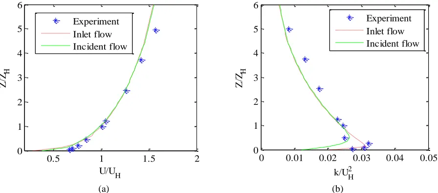
A rectangular computational domain, as shown in Figure 6, was created for the CFD simulation based on the recommendations by AIJ guidelines [65] and [21, 66]. The domain width, length, and height were 2.12 𝑚 × 3.28 𝑚 × 0.96 𝑚, respectively. Moreover, ICEM CFD was used to create a structured hexahedral mesh around and inside the building model. An O-grid block with first-layer size of 1 × 10−4 𝑚 was used for the solid walls, resulting to an average y+ ≈ 1. No-slip boundary condition was considered for all solid walls with aerodynamically smooth surfaces. The symmetric wall boundary condition was also applied to the lateral and top boundaries, and a zero static pressure was assigned to the outlet plane. The inlet vertical velocity in addition to the turbulent kinetic energy profiles were adapted from the experiment by Tominaga and Blocken [13] (see Figure 7) to mock the condition at the lower part of a neutral atmospheric boundary layer:

𝑈(𝑧) 𝑈𝐻 = (

𝑧 𝐻)

0.25 ₍₂₀₎

where 𝑈(𝑧) is the streamwise velocity at the height of 𝑧, and 𝑈_𝐻= 4.3 𝑚 𝑠⁄ is the reference velocity at the building height 𝐻. The measured vertical profile of the TKE was also approximated by an exponential formulation [13] while the turbulent kinetic energy dissipation rate 𝜀(𝑧) was approximated in accordance with the AIJ guidelines [65]:

𝑘(𝑧) 𝑈𝐻2

= 0.033 𝑒𝑥𝑝−0.32(𝑧 𝐻⁄ ) (21)

𝜀(𝑧) = 𝐶_𝜇12𝑘(𝑧)𝑈𝐻 𝐻 𝛼 (

𝑧 𝐻)

𝛼−1 ₍₂₂₎

14

(a) (b)

Figure 6 (a) Computational domain and (b) computational grid around the building surfaces.

(a) (b)

Figure 7 Vertical profiles of (a) the time averaged velocity and (b) turbulent kinetic energy of the experiment for the inlet flow and the incident flow in an empty-domain test case

3. Result and Discussion 3.1 Mesh Independency Study

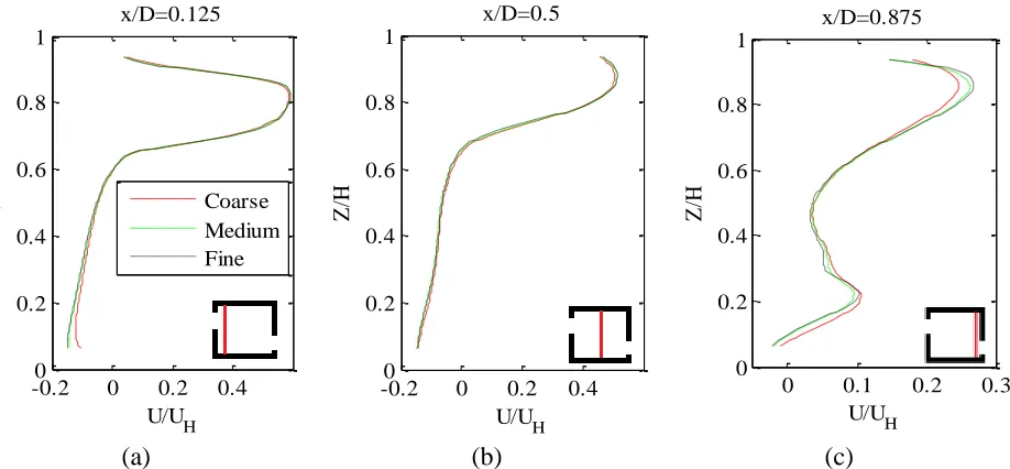
In order to find an independent mesh from the cell sizes, a sensitivity analysis was firstly conducted with three different cell numbers of 668,050; 1,231,824; and 2,271,371. Building configuration of case B (see Figure 4) was selected for the mesh independency study. In Figure 8, the profiles of the streamwise velocity are shown on the vertical plane at 𝑥_𝐷= 0.125, _𝐷𝑥= 0.5,

𝑎𝑛𝑑 _𝐷𝑥 = 0.875. It can be seen that the difference between the fine and medium meshes is negligible, thus the later mesh was chosen for the rest of the CFD simulations in this study.

0.5 1 1.5 2

0 1 2 3 4 5 6

U/U_H

Z

/ZH

Experiment Inlet flow Incident flow

0 0.01 0.02 0.03 0.04 0.05 0

1 2 3 4 5 6

k/U_H2

Z

/Z H

Experiment Inlet flow Incident flow

0.96m

3.28m

15

(a) (b) (c)

Figure 8 Vertical profiles of the streamwise velocity on the vertical plane at (a) 𝒙/𝑫 = 𝟎. 𝟏𝟐𝟓, (b) 𝒙/𝑫 = 𝟎. 𝟓, and (c) 𝒙/𝑫 = 𝟎. 𝟖𝟕𝟓.

3.2 CFD Validation

For the validation study, performance of five commonly used turbulence models, including the standard 𝑘 − 𝜀, 𝑅𝑁𝐺 𝑘 − 𝜀, 𝑘 − 𝜔, 𝑆𝑆𝑇 and 𝐵𝑆𝐿 𝑅𝑆𝑀, were compared in terms of airflow rate and validation metrics for the velocity field.

3.2.1 Airflow Rate

As shown in Figure 9, the CFD predictions of the non-dimensional airflow rate (_𝐴𝑄

𝑜𝑈𝐻) for different opening configurations and turbulence models are compared with the experimental results by Tominaga and Blocken [13]. It can be seen that the airflow rate demonstrates a relationship with the openings height. The highest experimentally measured airflow was reported for Case A where both windward and leeward openings are placed at the upper half of the building height close to the roof. Inversely, the lowest airflow rate was measured in cases C and D where the windward opening is close to the ground. The windward opening in case A is located near the stagnation point of the building, exposing to a higher wind surface pressure and free stream velocity, and therefore resulting in a higher airflow rate. In contrast, for cases C and D, not only the wind surface pressure around the windward opening is low, but the entering velocity is also low due to the lower height of the windward opening; hence, these cases correspond to the lowest airflow rates.

-0.20 0 0.2 0.4 0.2

0.4 0.6 0.8 1

U/U_H

Z

/H

x/D=0.125

Coarse Medium Fine

-0.20 0 0.2 0.4 0.2

0.4 0.6 0.8 1

U/U_H

Z

/H

x/D=0.5

0 0.1 0.2 0.3 0

0.2 0.4 0.6 0.8 1

U/U_H

Z

/H

16

Figure 9Airflow rate prediction by CFD models in comparison with the experimental results by Tominaga and Blocken [13]

In order to compare the CFD and experimental results, the lower and upper bounds of the measured airflow rate are also depicted in Figure 9, which are obtained based on a ±7% uncertainty of the tracer gas method reported by [13]. Comparing the airflow rate predictions by CFD and those of the measurement reveals that the accuracy of all turbulence models are acceptable for cases C, D, and E as the predicted values are within the upper and lower bounds. Nonetheless, for cases A and B, where windward opening is located at the upper height of the building near the stagnation point, the calculated airflow rate with all turbulence models are out of the expected range of the experiment. The relative error in prediction of the airflow rate for case A is about 20% for the 𝐵𝑆𝐿 𝑅𝑆𝑀, 𝑅𝑁𝐺, and 𝑆𝑆𝑇 models and 23% and 25% for the standard 𝑘 − 𝜀 and 𝑘 − 𝜔 models, respectively.

For case B, the relative error for the standard 𝑘 − 𝜀, 𝑘 − 𝜔, 𝑆𝑆𝑇 and 𝑅𝑁𝐺 models is about 10% while the 𝐵𝑆𝐿 𝑅𝑆𝑀 shows the lowest error of about 7%. The low accuracy of the RANS models in prediction of the airflow rate for cases A and B is associated to the poor accuracy of the steady RANS models in estimation of the flow behavior in the stagnation point over the windward façade. Moreover, incapability of the steady RANS models in prediction of the unsteady behavior of the flow around the building and the entering jet near the windward opening inside the building results in a lower accuracy for the CFD models of cases A and B. As demonstrated in [13], the flapping behavior and the Kelvin–Helmholtz instability formation are very strong in cases A and B, which cannot be captured by the steady RANS models. In contrast, the flapping behavior of the entering jet and the Kelvin–Helmholtz instability are noticeably decreased in

𝑄 𝐴_𝑜1𝑈_𝐻

17

cases C and D where the windward opening is closer to the floor, and hence, more accurate CFD predictions are obtained for these two cases.

3.2.2 Velocity Field

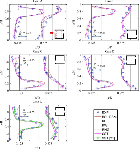
Vertical profiles of the streamwise velocity 𝑈 _𝑈 𝐻

⁄ on the vertical plane at streamwise positions 𝑥

𝐷

⁄ = 0.125 and 𝑥⁄ = 0.875_𝐷 close to the windward and leeward openings are illustrated in

Figure 10. Numerical results for all opening configurations are compared with the experimental

results by Tominaga and Blocken [13]; for case E, the numerical results are also compared with the numerical results by van Hooff, Blocken and Tominaga [21]. For case A, in which both openings are located at the upper half of the building height close to the roof, the entering jet

through the windward opening has the maximum velocity ratio of 𝑈𝑚𝑎𝑥 _𝑈 𝐻

⁄ = 0.75. The jet

momentum is weakened as it moves toward the leeward opening where the jet velocity ratio

becomes 𝑈𝑚𝑎𝑥 _𝑈 𝐻

⁄ = 0.45. For case A, all turbulence models present acceptable results for the

vertical velocity profiles. The 𝑆𝑆𝑇 and 𝑅𝑁𝐺 models, however, over-predict the jet velocity at the windward and leeward openings, and under-predict the recirculation flow at the middle of the building surface close to the windward opening. The velocity of the entering jet for case B is

𝑈_𝑚𝑎𝑥 𝑈_𝐻

⁄ = 0.5, which is apparently lower than the case A, despite having the same height for the

windward opening. In case B, as demonstrated in [13], the airflow encounters a larger resistance inside the building in comparison with case A, because the entering jet impinges on the opposite wall, and then redirects toward the leeward opening near the floor. In this case, the outlet jet

velocity ratio is noticeably decreased to 𝑈𝑚𝑎𝑥 _𝑈 𝐻

⁄ = 0.11. This implies the reason for the higher

airflow rate for case A, which is 1.4 times larger than the one measured in case B. The accuracy of all turbulence models is observed to be reasonable for case B; however, they all overestimate the recirculating flow close to the floor at 𝑥⁄ = 0.125_𝐷 .

For case C, the entering jet has a lower velocity than cases A and B. This is mainly due to the lower pressure difference across the openings, and also the lower velocity at the opening height

in comparison with cases A and B. The measured jet velocity for this case is about 𝑈𝑚𝑎𝑥 _𝑈 𝐻

⁄ =

0.4, but all CFD models over-estimate the value between 0.5 and 0.6. The estimated streamwise velocity profile by the RANS models is generally very close to the experiment. A same outlet jet

velocity about 𝑈𝑚𝑎𝑥 _𝑈 𝐻

⁄ = 0.25 is obtained by all turbulence models similar to the experiment.

Case D has almost a same entering jet velocity as case C, but the outlet jet has a considerably

lower velocity of 𝑈𝑚𝑎𝑥 _𝑈 𝐻

⁄ = 0.1 as the flow is directed upward to the leeward opening. The

18

Figure 10 Vertical profiles of the streamwise velocity on the vertical plane at 𝒙/𝑫 = 𝟎. 𝟏𝟐𝟓 and 𝒙/𝑫 = 𝟎. 𝟖𝟕𝟓 for different turbulence models.

The measured velocity jet for case E with two openings at the mid height of the building was reported to be about 0.43, but it is again overestimated by all turbulence models in a range between 0.50 and 0.58. At the leeward opening, the velocity is decreased to a half value predicted in the windward jet. Numerical results provided by van Hooff, Blocken and Tominaga [21] are also depicted for the 𝑆𝑆𝑇 turbulence model, which is again very close to the simulation results. The velocity vector near the leeward opening is generally under-predicted by the 𝑆𝑆𝑇 and 𝑅𝑁𝐺 models.

0.125 0.875 0 0.2 0.4 0.6 0.8 1 x/D z/ H Case A 0.125 0.875 0 0.2 0.4 0.6 0.8 1 x/D z/ H Case B 0.125 0.875 0 0.2 0.4 0.6 0.8 1 x/D z/ H Case C 0.125 0.875 0 0.2 0.4 0.6 0.8 1 x/D z/ H Case D 0.125 0.875 0 0.2 0.4 0.6 0.8 1 x/D z/ H Case E 𝑈

𝑈𝐻= 0.25

𝑈 𝑈𝐻= 0.25

𝑈

𝑈𝐻= 0.25 _𝑈

𝑈𝐻= 0.25

19

In order to have more precise view on the accuracy of the CFD model, the fraction of the predictions within a factor of 2 of the observations (𝐹𝐴𝐶2) are calculated for the velocity field over the 63 measurement points inside the building (see Figure 4). The FAC2 metric is defined as below:

𝐹𝐴𝐶2 = 1 𝑁∑ 𝑛𝑖

𝑁

𝑖=1

𝑖𝑓 0.5 ≤ 𝑃𝑖

𝑄𝑖 ≤ 2 𝑛𝑖 = 1 𝑒𝑙𝑠𝑒 𝑛𝑖 = 0 (23) where 𝑄𝑖 and 𝑃𝑖 are the measured and computed values of the streamwise velocity for sample 𝑖, respectively. 𝑁 = 63 is the number of measurement points. The ideal value for a complete agreement between the experiments and numerical results is 𝐹𝐴𝐶2 = 1.

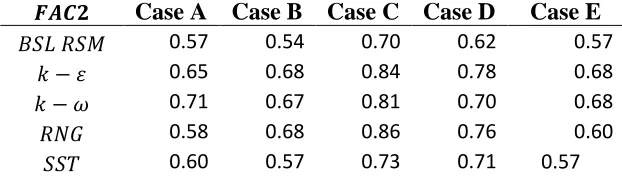
As shown in Table 2, for all turbulence models and opening configurations, the value of 𝐹𝐴𝐶2 is larger than the threshold of 𝐹𝐴𝐶2 ≥ 0.5 [67]. The highest agreement between the CFD and experimental results is obtained for cases C and D with 𝐹𝐴𝐶2 > 0.7 against all turbulence models except the 𝐵𝑆𝐿 𝑅𝑀𝑆 for case D where 𝐹𝐴𝐶2 = 0.62. The accuracy of the CFD model in prediction of the velocity profile for cases A, B and E shows almost same values; however, as shown in Figure 9, the accuracy of the CFD model in estimating the airflow rate was beyond the measurement uncertainty in cases A and B.

Table 2 Validation metrics for the streamwise velocity (_𝑼𝑼

𝑯) for different turbulence models

𝑭𝑨𝑪𝟐 Case A Case B Case C Case D Case E

𝐵𝑆𝐿 𝑅𝑆𝑀 0.57 0.54 0.70 0.62 0.57

𝑘 − 𝜀 0.65 0.68 0.84 0.78 0.68

𝑘 − 𝜔 0.71 0.67 0.81 0.70 0.68

𝑅𝑁𝐺 0.58 0.68 0.86 0.76 0.60

𝑆𝑆𝑇 0.60 0.57 0.73 0.71 0.57

3.3 Variation of the Airflow Rate for Different Building Configurations

In Figure 11, the variation of the non-dimensional airflow rate through the windward opening, average internal pressure coefficient (𝐶_𝑃𝑖), and the local pressure difference between windward

and leeward openings (∆𝐶𝑃 = 𝐶𝑃1𝐸𝑥𝑝− 𝐶𝑃2𝐸𝑥𝑝) are plotted for five different opening positions defined as cases A, B, C, D and E, and three building configurations (i.e. square cube, cuboid, and long corridor). The relative position of the windward and leeward openings is also shown in Figure 4.

20

located close to the ground (case B), the mean internal pressure noticeably increases while the wind surface pressure inversely decreases, and thus the airflow rate decreases relative to case A.

For cases C and D, in which the windward opening is located close to the ground, the airflow rate further decreases. In these cases, despite having the lowest internal pressure, the free stream velocity is significantly lower at the windward opening height. Furthermore, the wind surface pressure is noticeably lower than other cases (see Fig.11_c). Comparing to cases C and D, the airflow rate increases in case E for all three building models while the internal and wind surface pressures elevate as well. The trends of the airflow rate variation for the square cube and cuboid buildings are very similar, but the long corridor model is quite less sensitive to the openings position. This is mainly due to the lower wind surface pressure gradient over the windward and leeward surfaces of this building model (Fig.11_c).

(a)

(b) (c)

Figure 11 Effect of the openings position and building geometry on (a) the non-dimensional airflow rate at the windward opening (b) the mean internal pressure (c) the local wind surface pressure difference.

Case A Case B Case C

Case D Case E

𝑄

𝐴𝑜1 𝑈𝐻

∆

21

3.4 Factor Screening for Fitting the Model Approximation for 𝐂_𝐝∗

A total number of 250 samples (CFD simulations) were generated for each building model (i.e. square cube, cuboid, and long corridor buildings) using the methodology that was described in

Figure 3. In Figure 12, the histogram of the adaptive discharge coefficient (𝐶_𝑑∗) for the square cube,

cuboid and long corridor buildings is shown. The values of 𝐶_𝑑∗ for the square cube and cuboid buildings are changing between 0.47 ≤ 𝐶_𝑑∗ ≤ 0.78 and 0.41 ≤ 𝐶_𝑑∗ ≤ 0.83, respectively. For the long corridor model, the 𝐶_𝑑∗ variation is smaller than the other building models with a value between 0.46 and 0.63. The mean value of 𝐶_𝑑∗ over 250 samples for each building model is also shown in Figure 12. These values for square cube, cuboid, and long corridor buildings are 0.57, 0.62, and 0.56, respectively. The standard deviation of 𝐶_𝑑∗ is respectively 0.05, 0.06, and 0.03 for square cube, cuboid, and long corridor buildings. It is evident that the long corridor building not only has the lowest mean value of 𝐶_𝑑∗, but it also does have the lowest standard deviation.

Figure 12 Histogram of discharge coefficent for square cube, cuboid, and long corridor building models.

The first step in fitting and analyzing the RSM for the adaptive discharge coefficient (𝐶_𝑑∗) is to identify factors that have the most influence on the variation of 𝐶_𝑑∗. This process is called factor screening or characterization [68], and was performed for 250 samples for each building model.

In Figure 13, the Pareto chart of standardized effects on 𝐶_𝑑∗ is shown for the square cube, cuboid

and long corridor building models. The Pareto chart shows the relative magnitude and statistical significance of input parameters on the output response [69]. The reference line on the charts indicates which effects are significant; factors are considered significant when their effects are larger than the reference line. Thus, all the factors that have less effect than the reference line are considered insignificant.

22

analysis. It can be observed that, for all building geometries, the most effective factor on the discharge coefficient is the vertical position of the windward opening (𝐻_𝑤). For the square cube and cuboid building shapes, the variation of the leeward opening position (𝐻_𝑙) has a significant effect on the 𝐶_𝑑∗ variation, but in contrast, for the long corridor building model, 𝐶_𝑑∗ is less sensitive to the leeward opening position. Correlation effects up to the 2nd-order are significant for the three building models, but all of the 3rd-order correlations are insignificant.

(a) (b) (c)

Figure 13 Pareto chart of standardized effects of 𝑪𝒅∗ for (a) square cube, (c) cuboid, and (c) long corridor building

models.

3.5 Results of the Cross-validation Study for Model Approximations of 𝐂_𝐝∗

23

The average errors of the Quadratic and Cubic models are 0.074 and 0.071, respectively. The Quartic model shows an average-error of about 0.075. A lower average-error is obtained for the RBF models with a value of 0.064 and 0.054 for the models with 90 and 220 samples, respectively. The calculated maximum-error of all model approximations is very close to each other and is in the range of 0.41 to 0.44. The root-mean-square (RMS) errors of the Quadratic and Quartic models are equal to 0.107. The lowest RMS-error is predicted for the RBF2 model, which is about 0.098. It can be seen that, the RBF2 model provides the highest accuracy for the model approximation of 𝐶_𝑑∗, hence, it was selected for creating the correlation for the adaptive discharge coefficient. Similar results were found for the square cube and long corridor building models. After tuning the obtained correlation and its individual terms, a final correlation for 𝐶_𝑑∗ was generated for each building model. The coefficients of the developed approximations for the adaptive discharge coefficient are available on request.

Table 3 Cross-validation study for model approximations of 𝑪𝒅∗ over 30 samples

Model approximation

Number of training samples

Average error

Maximum error

RMS error

RSM Quadratic 28 0.074 0.423 0.107

RSM Cubic 34 0.071 0.416 0.106

RSM Quartic 40 0.075 0.412 0.107

RBF1 90 0.064 0.448 0.102

RBF2 220 0.054 0.443 0.098

3.6 Accuracy of the AFN Model for Adaptive Discharge Coefficient 𝐂_𝐝∗

24

the surface wind pressure on the windward and leeward surfaces is not as high as those for other two building models. Thus, using the local-surface wind pressure instead of the surface-averaged wind pressure does not improve the accuracy of the orifice-based model.

When the orifice-based model is used with the local-surface wind pressure and adaptive discharge coefficient (𝐶_𝑑∗) as a function of the openings’ geometry and position, the relative error of the airflow rate is seen to be considerably lower than the cases with constant 𝐶_𝑑. The minimum and maximum errors of the airflow rate with the adaptive discharge coefficient using the RBF2 correlation for the square cube, cuboid and long corridor buildings are found to be -5.8%, -4.9%, -1.2% and 8.8%, 4.8%, 1.2%, respectively. This apparently shows that assuming a constant discharge coefficient for the cross-ventilation scenarios considerably decreases the accuracy of the orifice-based equation for the wall porosity range between 3% and 25%.

25

The relative errors of the airflow rate calculated by the modified orifice-based equation for cases A, B, C, D and E compared to the experimental results by Tominaga and Blocken [13] are plotted in Figure 15. For all opening configurations, the relative error of using the surface-averaged wind pressure and constant 𝐶_𝑑 is larger than those obtained from the local-surface wind pressure; the values are found to be 45.5%, 25.4%, 12.4%, 8.4% and 19.4% for cases A, B, C, D and E, respectively. The relative error of the orifice-based equation with the local-surface wind pressure and constant 𝐶_𝑑 is estimated to be 38.3%, 16.5%, 6.4%, 0.8%, and 8.8% for cases A, B, C, D and E, respectively. The CFD simulation error for all cases except case D is found to be less than those estimated with using the local-surface wind pressure and constant discharge coefficient.

When the local-surface wind pressure with the adaptive discharge coefficient is used in the orifice-based equation, the error of the airflow rate estimation is considerably reduced to 22.8%, 8.1%, 3.3%, 7.4% and 7.3% for cases A, B, C, D and E, respectively. The significant increase in the accuracy of the orifice-based model using the adaptive discharge coefficient can be observed for all opening configurations in Figure 15. The highest value of 𝐶_𝑑∗ is obtained for case A where 𝐶_𝑑∗ _{= 0.77 followed by case B with 𝐶}

𝑑∗ = 0.66. For cases C and E, the value of 𝐶𝑑∗ is found to be 0.62 and 0.61, respectively. The lowest value of 𝐶_𝑑∗ = 0.56 is calculated for case C.

Figure 15 Relative error of the airflow rate calculation based on the orifice-based equation and CFD model for different opening configurations in comparison with the experiment by Tominaga and Blocken [13]

3.7 Conclusion

The application of the orifice-based model utilized in AFN model for the cross-ventilation of unsheltered building models was discussed for different building geometries and different opening configurations. It was shown that, assuming a constant value for the discharge

𝐶_𝑑∗_{= 0.77}

𝐶𝑑∗= 0.66

𝐶𝑑∗= 0.62 𝐶𝑑∗= 0.56

26

coefficient for the openings results in a noticeable inaccuracy of the orifice-based model in prediction of the airflow rate. A modified and adaptive discharge coefficient (𝐶_𝑑∗) was therefore proposed, which is a function of the building and openings geometries and vertical positions. The modified discharge coefficient was obtained by utilizing statistical methods and meta-model approximations for three different building configurations, including square cube, cuboid, and long corridor scenarios. A CFD model was, at first, validated using an experimental study, and then a database was generated for different opening positions by varying the building and openings’ geometry and vertical position. The calculated airflow rate from the CFD model alongside the local-surface wind pressure from the experiment was passed into the orifice-based model to define the adaptive discharge coefficient. The accuracy of the proposed discharge coefficient correlation was discussed by comparing the airflow rate results with the CFD and experiment for a cuboid building model. The following findings can be addressed as the main conclusions of this study:

- The accuracy of CFD and the orifice-based models varies for different opening configurations; the highest discrepancy occurs when the windward opening is close to the roof with relative errors of 20% and 45.5% for the CFD model and the orifice-based model with surface-averaged wind pressure and constant discharge coefficient, respectively.

- The accuracy of the orifice-based model for the square cube and cuboid buildings can be improved by using the local-surface wind pressure instead of the surface-averaged wind pressure. However, the long corridor building model is less sensitive to the surface wind pressure gradient over the windward and leeward openings.

- The highest airflow rate can be obtained when the windward opening is close to the roof for the square cube and cuboid buildings. In contrast, for the long corridor building, the airflow rate variation with the opening positions is smaller than other building models. - The accuracy of the orifice-based model can be considerably increased when the

modified and adaptive discharge coefficient is used instead of a constant value, which is a default value in the AFN model embedded in EnergyPlus; the relative error of the airflow rate can be decreased from 38% to 22% for case A and from 16.5% to 8.0% for case B.

Despite the noticeable improvement shown in this study for the prediction of the cross-ventilation airflow rate, accuracy of the CFD and orifice-based model using the modified discharge coefficient is still lower than the measurement uncertainty when both windward and leeward opening are close to the roof (Case A and B). Further study, hence, is required to investigate the performance of the RANS models for the situations where the openings are close to the stagnation point on the windward façade. Future works will be focused to extent the proposed methodology for other wind angles and also to consider the sheltering effects.

Acknowledgment

27 References

[1] C.A. Balaras, A.G. Gaglia, E. Georgopoulou, S. Mirasgedis, Y. Sarafidis, D.P. Lalas, European residential buildings and empirical assessment of the Hellenic building stock, energy consumption, emissions and potential energy savings, Building and Environment 42(3) (2007) 1298-1314.

[2] H.-x. Zhao, F. Magoulès, A review on the prediction of building energy consumption, Renewable and Sustainable Energy Reviews 16(6) (2012) 3586-3592.

[3] K. Kumaran, Heat, air and moisture transfer in insulated envelope parts, Final report 3 (1996). [4] B. Wang, T. Dogan, D. Pal, C. Reinhart, Simulating naturally ventilated buildings with detailed CFD-based wind pressure database, (2012).

[5] Z. Cheng, L. Li, W.P. Bahnfleth, Natural ventilation potential for gymnasia – Case study of ventilation and comfort in a multisport facility in northeastern United States, Building and Environment 108 (2016) 85-98.

[6] P. Prajongsan, S. Sharples, Enhancing natural ventilation, thermal comfort and energy savings in high-rise residential buildings in Bangkok through the use of ventilation shafts, Building and Environment 50 (2012) 104-113.

[7] Y.C. Aydin, P.A. Mirzaei, Wind-driven ventilation improvement with plan typology alteration: A CFD case study of traditional Turkish architecture, Building Simulation, Springer, 2017, pp. 239-254. [8] P. Karava, Airflow prediction in buildings for natural ventilation design: wind tunnel measurements and simulation, Concordia University, 2008.

[9] D. Etheridge, A perspective on fifty years of natural ventilation research, Building and Environment 91 (2015) 51-60.

[10] N. Khan, Y. Su, S.B. Riffat, A review on wind driven ventilation techniques, Energy and Buildings 40(8) (2008) 1586-1604.

[11] M. Sandberg, Wind induced airflow through large openings: summary, International Energy Agency Annex 35 (2002).

[12] Y. Tominaga, B. Blocken, Wind tunnel experiments on cross-ventilation flow of a generic building with contaminant dispersion in unsheltered and sheltered conditions, Building and Environment 92 (2015) 452-461.

[13] Y. Tominaga, B. Blocken, Wind tunnel analysis of flow and dispersion in cross-ventilated isolated buildings: impact of opening positions, Journal of Wind Engineering and Industrial Aerodynamics 155 (2016) 74-88.

[14] G. Carrilho da Graça, N.C. Daish, P.F. Linden, A two-zone model for natural cross-ventilation, Building and Environment 89 (2015) 72-85.

[15] T. Kurabuchi, M. Ohba, T. Goto, Y. Akamine, T. Endo, M. Kamata, Local Dynamic Similarity Concept as Applied to Evaluation of Discharge Coefficients of Cross-Ventilated Buildings-Part 1 Basic Idea and Underlying Wind Tunnel Tests; Part 2 Applicability of Local Dynamic Similarity Concept; Part 3 Simplified Method for Estimating Dynamic Pressure Tangential to Openings of Cross-Ventilated Buildings,

International Journal of Ventilation 4(3) (2005) 285.

[16] M. Ohba, T. Kurabuchi, E. Tomoyuki, Y. Akamine, M. Kamata, A. Kurahashi, Local Dynamic Similarity Model of Cross-Ventilation Part 2-Application of Local Dynamic Similarity Model, International Journal of Ventilation 2(4) (2004) 383-394.

[17] C.-R. Chu, B.-F. Chiang, Wind-driven cross ventilation in long buildings, Building and Environment 80 (2014) 150-158.

28

[19] T. Norton, J. Grant, R. Fallon, D.-W. Sun, Improving the representation of thermal boundary conditions of livestock during CFD modelling of the indoor environment, Computers and Electronics in Agriculture 73(1) (2010) 17-36.

[20] M. Teitel, G. Ziskind, O. Liran, V. Dubovsky, R. Letan, Effect of wind direction on greenhouse ventilation rate, airflow patterns and temperature distributions, Biosystems Engineering 101(3) (2008) 351-369.

[21] T. van Hooff, B. Blocken, Y. Tominaga, On the accuracy of CFD simulations of cross-ventilation flows for a generic isolated building: comparison of RANS, LES and experiments, Building and Environment (2016).

[22] Y.-H. Chiu, D. Etheridge, Experimental technique to determine unsteady flow in natural ventilation stacks at model scale, Journal of wind engineering and industrial aerodynamics 92(3) (2004) 291-313. [23] L. Ji, H. Tan, S. Kato, Z. Bu, T. Takahashi, Wind tunnel investigation on influence of fluctuating wind direction on cross natural ventilation, Building and Environment 46(12) (2011) 2490-2499.

[24] Y. Jiang, D. Alexander, H. Jenkins, R. Arthur, Q. Chen, Natural ventilation in buildings: measurement in a wind tunnel and numerical simulation with large-eddy simulation, Journal of Wind Engineering and Industrial Aerodynamics 91(3) (2003) 331-353.

[25] L.J. Lo, A. Novoselac, Cross ventilation with small openings: Measurements in a multi-zone test building, Building and Environment 57 (2012) 377-386.

[26] J.S. Park, Long-term field measurement on effects of wind speed and directional fluctuation on wind-driven cross ventilation in a mock-up building, Building and Environment 62 (2013) 1-8.

[27] M.H. Sherman, I.S. Walker, M.M. Lunden, Uncertainties in air exchange using continuous-injection, long-term sampling tracer-gas methods, International Journal of Ventilation 13(1) (2014) 13-28.

[28] S. Kato, Flow network model based on power balance as applied to cross-ventilation, International journal of ventilation 2(4) (2004) 395-408.

[29] G.N. Walton, AIRNET: a computer program for building airflow network modeling, National Institute of Standards and Technology Gaithersburg, MD, USA1989.

[30] U. DoE, Energyplus engineering reference, The reference to energyplus calculations (2010). [31] P. Karava, T. Stathopoulos, A.K. Athienitis, Wind-induced natural ventilation analysis, Solar Energy 81(1) (2007) 20-30.

[32] S. Kato, S. Murakami, A. Mochida, S.-i. Akabayashi, Y. Tominaga, Velocity-pressure field of cross ventilation with open windows analyzed by wind tunnel and numerical simulation, Journal of Wind Engineering and Industrial Aerodynamics 44(1-3) (1992) 2575-2586.

[33] H. Breesch, A. Janssens, Performance evaluation of passive cooling in office buildings based on uncertainty and sensitivity analysis, Solar energy 84(8) (2010) 1453-1467.

[34] D. Costola, B. Blocken, J. Hensen, Overview of pressure coefficient data in building energy simulation and airflow network programs, Building and Environment 44(10) (2009) 2027-2036. [35] D. Cóstola, B. Blocken, J. Hensen, Uncertainties due to the use of surface averaged wind pressure coefficients, Proceedings of the 29th AIVC Conference, Kyoto, Japan, 2008, pp. 14-16.

[36] J. Lim, Y. Akashi, R. Ooka, H. Kikumoto, Y. Choi, A probabilistic approach to the energy-saving potential of natural ventilation: Effect of approximation method for approaching wind velocity, Building and Environment 122 (2017) 94-104.

[37] J. Lim, R. Ooka, H. Kikumoto, Effect of diurnal variation in wind velocity profiles on ventilation performance estimates, Energy and Buildings 130 (2016) 397-407.

[38] F. Monari, P. Strachan, Characterization of an airflow network model by sensitivity analysis: parameter screening, fixing, prioritizing and mapping, Journal of Building Performance Simulation 10(1) (2017) 17-36.

29

[40] S. Murakami, Wind tunnel test on velocity-pressure field of cross-ventilation with open windows, ASHRAE transactions 97 (1991) 525-538.

[41] M. Ohba, T. Kurabuchi, Y. Fugo, T. Endo, Local similarity model of cross-ventilation Part 2

Application, The 8th international conference on air distribution in rooms ‘ROOMVENT, 2002, pp. 617-620.

[42] C.R. Chu, Y.-H. Chiu, Y.-J. Chen, Y.-W. Wang, C.-P. Chou, Turbulence effects on the discharge

coefficient and mean flow rate of wind-driven cross-ventilation, Building and Environment 44(10) (2009) 2064-2072.

[43] T. Sawachi, N. Ken-ichi, N. Kiyota, H. Seto, S. Nishizawa, Y. Ishikawa, Wind pressure and air flow in a full-scale building model under cross ventilation, International Journal of Ventilation 2(4) (2004) 343-357.

[44] A.F. Handbook, American society of heating, refrigerating and air-conditioning engineers, Inc.: Atlanta, GA, USA (2009).

[45] M.W. Liddament, Air infiltration calculation techniques: An applications guide, Air Infiltration and Ventilation Centre Berkshire, UK1986.

[46] M. Grosso, Wind pressure distribution around buildings: a parametrical model, Energy and Buildings 18(2) (1992) 101-131.

[47] B. Knoll, J. Phaff, W. De Gids, Pressure simulation program, Implementing the Results of Ventilation Research, 16th AIVC conference, 19-22 September 1995, Palm Springs, USA, TNO, 1995.

[48] M. Swami, S. Chandra, Correlations for pressure distribution on buildings and calculation of natural-ventilation airflow, ASHRAE transactions 94(3112) (1988) 243-266.

[49] B. Wang, T. Dogan, D. Pal, C. Reinhart, SIMULATING NATURALLY VENTILATED BUILDINGS WITH DETAILED CFD-BASED WIND PRESSURE DATABASE, IBPSA-USA Journal 5(1) (2012) 353-360.

[50] R. Jin, W. Chen, A. Sudjianto, An efficient algorithm for constructing optimal design of computer experiments, Journal of Statistical Planning and Inference 134(1) (2005) 268-287.

[51] Y. Tamura, Aerodynamic database for low-rise buildings, Global Center of Excellence Program, Tokyo Polytechnic University, Database (2012).

[52] M.E. Johnson, L.M. Moore, D. Ylvisaker, Minimax and maximin distance designs, Journal of statistical planning and inference 26(2) (1990) 131-148.

[53] R.H. Myers, D.C. Montgomery, G.G. Vining, C.M. Borror, S.M. Kowalski, Response surface methodology: a retrospective and literature survey, Journal of quality technology 36(1) (2004) 53. [54] D.S. Broomhead, D. Lowe, Radial basis functions, multi-variable functional interpolation and adaptive networks, DTIC Document, 1988.

[55] E.J. Kansa, Motivation for using radial basis functions to solve PDEs, RN 64(1) (1999) 1.

[56] D. Cóstola, B. Blocken, M. Ohba, J. Hensen, Uncertainty in airflow rate calculations due to the use of surface-averaged pressure coefficients, Energy and Buildings 42(6) (2010) 881-888.

[57] T. Nozu, T. Tamura, Y. Okuda, S. Sanada, LES of the flow and building wall pressures in the center of Tokyo, Journal of Wind Engineering and Industrial Aerodynamics 96(10) (2008) 1762-1773.

[58] T. Yang, N. Wright, D. Etheridge, A. Quinn, A comparison of CFD and full-scale measurements for analysis of natural ventilation, International Journal of Ventilation 4(4) (2006) 337-348.

[59] P. Richards, S. Norris, Appropriate boundary conditions for computational wind engineering models revisited, Journal of Wind Engineering and Industrial Aerodynamics 99(4) (2011) 257-266.

[60] R. Akins, J. Peterka, J. Cermak, Averaged pressure coefficients for rectangular buildings, Wind Engineering 1 (1979) 369,380.

[61] G. Walton, W. Dols, CONTAM 2.1 Supplemental user guide and program documentation. 2006, Gaithersburg, MD: National Institute of Standards and Technology Google Scholar (2006).

30

[63] C.M. Rhie, W.L. Chow, Numerical study of the turbulent flow past an airfoil with trailing edge separation, AIAA Journal 21(11) (1983) 1525-1532.

[64] A. CFX, Solver Theory Guide. Ansys, Inc., Canonsburg, PA (2011).

[65] Y. Tominaga, A. Mochida, R. Yoshie, H. Kataoka, T. Nozu, M. Yoshikawa, T. Shirasawa, AIJ guidelines for practical applications of CFD to pedestrian wind environment around buildings, Journal of wind engineering and industrial aerodynamics 96(10) (2008) 1749-1761.

[66] P.A. Mirzaei, J. Carmeliet, Dynamical computational fluid dynamics modeling of the stochastic wind for application of urban studies, Building and Environment 70 (2013) 161-170.

[67] J. Franke, Best practice guideline for the CFD simulation of flows in the urban environment, Meteorological Inst.2007.